In this paper, we propose an approach to the problem of simultaneous shape and refractive index recovery from multispectral polarisation imagery captured from ...
Shape and Refractive Index Recovery from Single-View Polarisation Images Cong Phuoc Huynh1 Antonio Robles-Kelly1,2 Edwin R. Hancock3 1 RSISE, Bldg. 115, Australian National University, Canberra ACT 0200, Australia 2 National ICT Australia (NICTA) ∗, Locked Bag 8001, Canberra ACT 2601, Australia 3 Dept. of Comp. Science, The University of York, York YO105DD, UK
Abstract
tations. Reflectance models such as the Torrance-Sparrow model [19] and the Wolff model [24] can also be decomposed into polarisation components and are applicable to polarised light sources. In these models, the material properties and the geometry of the reflection process is expressed in a single equation with multiple degrees of freedom. As a result, the simultaneous recovery of the photometric and shape parameters becomes an underconstrained problem. To remedy the ill-posedness nature of the problem, Miyazaki et al. [13] assumed that the histogram of zenith angles of a given object is similar to that of a sphere so as to map the degree of polarisation to zenith angle. Using a similar experimental setup, which involves a spherical optical diffuser, Saito et al. [16] were able to recover the shape of transparent objects. Later, Atkinson and Hancock [1] published their work concerning the recovery of surface orientation from diffuse polarisation applied to smooth dielectric surfaces.
In this paper, we propose an approach to the problem of simultaneous shape and refractive index recovery from multispectral polarisation imagery captured from a single viewpoint. The focus of this paper is on dielectric surfaces which diffusely polarise light transmitting through the surface boundary into the air. The diffuse polarisation of the reflection process is modelled using a Transmitted Radiance Sinusoid curve and the Fresnel transmission theory. We provide a method of estimating the azimuth angle of surface normals from the spectral variation of the phase of polarisation. Moreover, to render the problem of simultaneous estimation of surface orientation and index of refraction well-posed, we enforce a generative model on the material dispersion equations for the index of refraction. This generative model, together with the Fresnel transmission ratio permits the recovery of the index of refraction and the zenith angle simultaneously. We show results on shape recovery and rendering for real world and synthetic imagery.
To overcome the difficulties in shape recovery from single images, the vision community has turned its attention to the use of multiple images for the recovery task. Rahmann and Canterakis [15] proposed a method based on polarization imaging for shape recovery of specular surfaces. Atkinson and Hancock [3] also made use of the correspondences between the phase and degree of polarisation in two views for shape recovery. Aiming to disambiguate the two possible zenith angles recovered from the degree of specular polarisation, Miyazaki et al. [11] analysed the derivative of the degree of polarisation while tilting the observed object by a small angle. As an alternative option to the use of multiple views, polarisation information can also be extracted from photometric stereo images for shape recovery. Using a similar experimental setup to photometric stereo, Thilak et al. [18] presented a nonlinear least-squares estimation algorithm to extract the complex index of refraction and the zenith angle of surface normals from multiple images illuminated by unpolarised light sources.
1. Introduction The polarisation of light is a property that describes the preferential orientation of oscillation of its electromagnetic field. Although the human vision system is oblivious to polarisation, their effects can be captured by devices such as polarimeters and more recently, polarisation cameras [25]. Such developments have broadened the applications of polarisation to areas such as target detection [9] and material property recovery [26]. Shape and material properties are usually co-existing factors that influence the appearance of an object to an observer and the polarisation properties of the emitted radiation. In an early discovery, Torrance, Sparrow and Birkebak [20] were able to measure the specular reflectance distribution of rough surfaces for different polarisation orien-
Its somewhat surprising that there is little work on the use of polarisation methods for the simultaneous estimation of surface orientation and photometric invariants, including
∗ National
ICT Australia is funded by the Australian Government’s Backing Australia’s Ability initiative, in part through the Australian Research Council.
1
index of refraction. Whereas material classification methods [6, 22] have been mainly interested in material intrinsic properties, they have often neglected the wavelength dependency of the index of refraction. In this paper, we propose a new approach to make this problem well-posed by using multispectral information from polarisation images taken from a single view point. In contrast to prior literature on polarisation methods for shape and material recovery, our work concentrates on the use of the Transmitted Radiance Sinusoid and Fresnel transmission theory so as to estimate the shape and refractive index simultaneously from polarisation images observed from a single viewpoint. This framework assumes little knowledge of the illumination conditions, as well as the material under study and the 3D surface orientation.
2. Shape and Refractive Index Recovery In this section, we present our method for the recovery of surface orientation and index of refraction from a set of polarisation images captured in a single view. Firstly, we commence by decomposing the given set of images into polarisation components. Next, we present an approach to estimating the azimuth angle of surface normals from the spectral phase angles. To complete the section, we show how to jointly estimate the zenith angle of the object surface normals and the refractive index of materials. The polarisation of light reflected from a surface can be measured by mounting a linear polariser in front of the camera’s optics. By rotating the polariser, one can capture polarisation components that are oriented at different angles in a plane orthogonal to the light propagation direction. The intensity captured at each image pixel varies sinusoidally with respect to the angle of rotation of the polariser. Specifically, at each pixel u and wavelength λ, the variation of the image intensity can be described by the following Transmitted Radiance Sinusoid (TRS) curve Imax − Imin Imax + Imin + cos(2ϑ − 2φ) 2 2 (1) where φ is the phase angle of polarisation of the reflected light, and Imin and Imax are the minimum and maximum intensities on the sinusoid at the pixel and wavelength of reference, respectively. Thus, at input, we have a set of N multispectral image cubes I(ϑ1 ), I(ϑ2 ), . . . , I(ϑN ), where the image I(ϑi ) has been acquired with the polariser’s transmission axis oriented at the ith step-angle with respect to a reference axis. We can index each of these images to wavelength λ ∈ {λ1 , . . . λK } by denoting Ii (u, λ) , I(u, λ, ϑi ) as the measured intensity at the pixel-site u and wavelength λ on the image I(ϑi ) corresponding to the ith polariser angle ϑi . I(u, λ, ϑ) =
2.1. Decomposing Polarisation Images There are several alternative methods of recovering the Imin , Imax and φ in Equation 1 from a successive sequence of polarisation images captured at several polariser angles. Note that Equation 1 contains three unknowns Imin , Imax and φ. Thus, by capturing the same scene with three or more polariser orientations, one can fit a sinusoidal curve through the intensity-polariser angle pairs using a numerical nonlinear least square fitting algorithm. This method is, however, not efficient since the optimisation has to be performed per pixel. Alternatively, these parameters can be obtained making use of the method in [25], where three images at 0◦ , 45◦ and 90◦ with respect to a reference axis are acquired so as to compute the phase, intensity and degree of polarisation. However, the method in [25] is susceptible to noise corruption since it employs only three images. Here, we employ an alternative that yields a stable estimation of the intensity, phase and degree of polarization by solving an overdetermined linear system of equations. The method is akin to that described by Nayar et al. in [14]. We commence by rewriting Equation 1 for each pixel-site u and wavelength λ in the following vector form T Imax +Imin 1 2 min Ii (u, λ) = cos(2ϑi ) Imax −I cos(2φ) 2 Imax −Imin sin(2ϑi ) sin(2φ) 2 =
fiT x
(2)
After collecting N ≥ 3 measurements at three or more polariser orientations, one arrives at the folllowing overdetermined linear system I = Ax
(3)
f1T I1 (u, λ) f2T I2 (u, λ) and A = where I = ... ... T IN (u, λ) fN Equation 3 is well-constrained since the number of equations N ≥ 3 is no less than the number of unknowns. Moreover, the coefficient matrix A depends solely on the polariser angle with respect to a direction in the image plane and, thus, allowing for an efficient solution of Equation 3 over all the image pixels and wavelengths simultaneously. Having obtained the solution for x = [x1 , x2 , x3 ]T , one can recover the maximal and minimal intensities on the sinusoid and the phase of polarisation at each pixel u and wavelength λ as q Imax = x1 + x22 + x23 q Imin = x1 − x22 + x23
φ
=
1 x3 arctan 2 x2
2.2. Estimation of the Azimuth Angle Now, we turn our attention to the estimation of the azimuth angle of the surface normals from the phase angles recovered above. Let us consider a diffuse reflection process from dielectric surfaces. In such a process, diffuse reflection takes place due to incicident light penetrating the surface and scattering within the dielectric body. We can safely assume that the internal scattering within the dielectric body is largely unpolarised, and that the diffusely emitted light from the surface occurs due to refraction through the material-air boundary. Further, the polarisation component oscillating parallel to the plane of reflection is the one that is refracted through the media-air surface boundary with the maximal efficiency. This can be explained by the fact that, the internally scattered light incident upon the material-air boundary is unpolarised and the Fresnel transmission component parallel to the reflection plane is always equal to or higher than the perpendicular component. In addition, the diffuse polarisation oriented at an arbitrary angle is a convex combination of its parallel and perpendicular oscillation components [21]. Furthermore, the maximal intensity on the TRS curve at pixel u and wavelength λ is reached at the phase angle φ. Thus, the azimuth angle α at pixel u is either the same as the phase of polarisation φ or differs from it by π [1], i.e. α(u) = φ or α(u) = φ ± π. To disambiguate the azimuth angle between the two possibilities, φ and φ±π, we assume convexity on the surface under observation. Under this assumption, surface normals point in the opposite direction to that of image gradients. One can determine the azimuth angle as the one between φ and φ ± π that yields the closer orientation to the negative gradient direction. However, across a broad spectrum, the estimated phase angle φ at a given pixel may vary widely. This is due to weak polarisation that causes a drift in phase angle estimation. Hence, the azimuth angle can be estimated as the weighted mean of the spectral phase of polarisation. The weights can be chosen to reflect the fitting error of the TRS curve to the intensity-polariser angle pairs at each wavelength. Here, the fitting error �(u, λ) is quantified as the L2 -norm of the residual �(u, λ) of the Equation 3, i.e. �(u, λ) = kI − Axk2 , where I, A and x have been computed per pixel and wavelength. The weight ω(u, λ) associated with the phase of polarisation at each wavelength is defined via a kernel weighting function. Here we employ the Epanechnikov kernel such that ( 1 − g(�(u, λ))2 if kg(.)k < 1 ω(u, λ) = (4) 0 otherwise 2
and h is a bandwidth paramewhere g(�(u, λ))2 = � (u,λ) h ter. Since the azimuth angle is a directional quantity, instead
of averaging the spectral phase angles directly, we estimate the mean of the sines and cosines of the spectral phase angles for each pixel-site as follows P sin(φ)ω(u, λ) λP hsin(φ)iλ = ω(u, λ) P λ cos(φ)ω(u, λ) λP hcos(φ)iλ = λ ω(u, λ) where h·iλ denotes the mean value across wavelengths. The estimated azimuth angle at pixel u then becomes hsin(φ)iλ if hcos(φ)iλ > 0 arctan( hcos(φ)iλ ) ∗ hsin(φ)i λ α (u) = arctan( hcos(φ)iλ ) + π if hcos(φ)iλ < 0 π if hcos(φ)iλ = 0 2
(5)
2.3. Joint Estimation of the Zenith Angle and Refractive Index In Section 2.2, we have shown how to estimate the azimuth angle of surface normals from the spectral phase of polarisation, and how to disambiguate between the azimuth candidate angles. To fully determine the surface shape, one needs to estimate the zenith angle of the surface normals with respect to the viewing direction. In this section, we will show how both the zenith angle and the material index of refraction can be recovered from the Fresnel ratio of diffuse polarisation. Note that, in prior literature, the degree of polarisation has been heavily exploited for the purpose of recovering the zenith angle of surface normals and the index of refraction [1, 2, 4, 11, 12, 18, 23]. However, there are a number of limitations that prevent the application of these methods in general uncontrolled and unpolarised lighting conditions for unknown shapes and materials. The main reason for this is that, these methods usually rely on either known index of refraction [1, 2, 4, 11, 12] or require many images to be captured in multiple views [11] or under several known light source directions [18]. The need for multiple measurements and complicated setups make them impractical for shape and material analysis on real-world data. Moreover, existing methods are limited by the kind of data at hand. With a single-band or trichromatic image, there is only a single equation relating the zenith angle and index of refraction through the degree of polarisation. Therefore, one is unable to estimate both of these quantities without further prior knowledge, such as known illumination directions or index of refraction. With an increasing number of wavelengths, i.e. image bands, we can utilise the correlation of the index of refraction across the whole spectrum making use of material dispersion equations. There are several approximating functions of dispersion in the physics literature. Of these, perhaps Cauchy’s and Sellmeier’s [5]
are the most popular. These equations allow the representation of the index of refraction with a few coefficients making use of a linear combination of rational functions of wavelength. As more samples are acquired at an increasing number of wavelengths, the number of equations exceeds the number of variables, rendering the problem solvable. Therefore, the recovery problem becomes well-constrained and can be formulated as a non-linear least square minimisation problem. In brief, the rationale behind our method lies in the use of dispersion equations, which, as we will show in our experiments, enforces constraints that replace the need for the prior knowledge on the index of refraction or illumination conditions. We focus on showing how the zenith angle and the material index of refraction are jointly estimated. Suppose that the imagery is acquired at K discrete sampled wavelengths λ ∈ {λ1 , . . . , λK }. As shown in Section 2.1, at each pixel location u and wavelength λ, we have already obtained the quantities Imax and Imin . Given unpolarised incident light, the maximal diffuse polarisation is observed in the direction parallel to the reflection plane, which also contains the reflected ray. The minimal diffuse polarisation is observed in the direction perpendicular to the reflected ray. This is a consequence of the developments presented in Section 2.2. Since the unpolarised incident light can be decomposed into incoherent polarisation components oscillating in the parallel and perpendicular planes with equal magnitudes, the polarisation components of the reflected light are proportional to the Fresnel transmission coefficients in the corresponding planes [5], i.e. Imin Imax
1 − F⊥ (u, λ) (6) 1 − Fk (u, λ) q 2 cos θ(u) n(u, λ)2 − sin2 θ(u) + sin2 θ(u) = n(u, λ)
=
where θ(u) is the zenith angle of the surface normal at location u, n(u, λ) is the refractive index of the same location at wavelength λ, and F⊥ (u, λ) and Fk (u, λ) are the perpendicular and parallel Fresnel reflectionq coefficients.
min as r(u, λ). At Let us denote the known quantity IImax each pixel location u, we solve the system of Equations 6 with λ ∈ {λ1 , . . . , λK } by converting it to a non-linear least square problem with the following cost function
E(u) =
q K � cos θ(u) n(u, λ )2 − sin2 θ(u) + sin2 θ(u) X i n(u, λi )
i=1
�2 − r(u, λi ) (7)
With the equation above in hand, we can provide further constraints on the index of refraction according to the Cauchy’s dispersion equation, as follows n(u, λ) =
M X
C1 (u)λ−2(k−1)
(8)
k=1
Here, the dispersion equation relates the index of refraction solely to the wavelength, with coefficients Ck (u), k ∈ {1, . . . , M } that are characteristic of the material. With this representation of n(u, λ), the cost function E(u) in Equation 7 can be reparameterised as a function of M + 1 variables, including θ(u) and Ck (u), k = 1, . . . , M . If the number of M dispersion coefficients is chosen such that M + 1 ≤ K, where K is the number of wavelengths, then the non-linear least square problem can be solved numerically by standard line-search or trust-region methods. Having obtained the azimuth and zenith angle of the surface normals, one can recover the shape under study by means of a surface integration method such as that in [8]. On the other hand, the index of refraction can be recovered from the dispersion equation making use of the dispersion coefficients Ck (u).
3. Experiments In this section, we perform experiments using our method for recovering surface orientation and refractive index on synthetic and real-world polarisation images. On the synthetic dataset, we provide the accuracy of our estimated parameters compared to their ground-truth. On the real-world images, we verify the accuracy of the recovered surface orientation and index of refraction through images rendered under novel lighting conditions. For all our experiments, we have set the bandwidth of the Epanechnikov kernel in Section 2.2 to unity. In addition, the form of Cauchy’s dispersion equation that we employ approximates the refractive index as an eighth-order rational function of wavelength, with five coefficients. The non-linear least square minimisation problem posed in Section 2.3 is solved by a subspace trust-region method that is based on the interiorreflective Newton method described in [7].
3.1. Synthetic Data We commence by performing experiments on a synthetic dataset. To build the dataset, we generate the 3D surface of a dome, a ridge, a torus, a volcano and a two-dome test shape. We render images of these synthetic shapes using the refractive index of 24 plastic and liquid materials reported in [10]. The image dataset is synthesized using the Wollf diffuse reflectance model for dielectrics [24] with the total diffuse albedo parameter being the spectral reflectance of Polyvinyl Chloride under ten illumination conditions. These amount
(a) L3
(b) L4
(c) L5
(f) 0◦
(g) 30◦
(h) 45◦
(d) L2 + L4 (e) L1 + L5
(i) 60◦
(j) 90◦
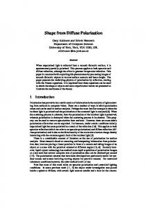
Figure 1. First row: Sample synthetic images of a dome rendered with the refractive index of Polystyrene under five different natural sunlight directions. Second row: Sample synthetic images of a test shape at five different angles of polarisation, under the frontal light source direction.
to a total of 1200 combinations of shape and photometric parameters. For each combination, five polarisation images are generated corresponding to five polariser orientations at 0◦ , 30◦ , 45◦ , 60◦ and 90◦ with respect to the vertical orientation in increments on the clockwise direction. All the multispectral images in our dataset are 30 bands in length, spanning the 430 − 720nm range, with a 10nm step between successive bands. The illuminants involved in the simulation lie in the same horizontal plane as the viewing direction. Each illuminant assumes one of five different directions pointing towards the surface under study. We have denoted these illuminants as L1 , L2 , L3 , L4 and L5 . These directions form angles of −26.5◦ , −14◦ , 0◦ , 14◦ and 26.5◦ with respect to the viewing direction, where a negative angle means the light direction is on the left-hand side of the view point and a positive angle means otherwise. In addition, each light assumes the power spectrum of either the natural sunlight or an incandescent light. The power spectrum of the two illuminant types have been acquired from sample light sources using a StellarNet spectrometer. The illuminant combinations used for this dataset include three instances of single illuminant directions, which are L3 , L4 and L5 , and two instances of two simultaneous illuminant directions which are L2 + L4 and L1 + L5 . In Figure 1, we show sample synthetic images generated for two shapes in the dataset. The first row shows the variation of shading with respect to the illumination direction, whereas the second row shows the variation of shading with respect to the angle of polarisation. The pseudocolour RGB images have been synthesized from the generated multispectral images using the Stiles and Burch colour matching function [17]. The images in the figure have been rendered with the refractive index of Polystyrene under the power spectrum of natural sunlight. In Figure 2, we present the shading and needle maps of
all the simulated shapes under the oblique light direction originating from the right-hand side of the viewing direction, at an angle of 26.5◦ (L5 ). The top row shows the input images, corresponding to the vertical polarisation direction. The middle and bottom rows show the recovered diffuse maps and needle-maps of the shapes on the top panels. Note that the surface geometry has been successfully recovered everywhere except for totally dark shadows, irrespective of shading variations. Furthermore, the figure shows that our method results in needle maps highly consistent with the test shapes. Here, the horizontal symmetry of the recovered shading and needle maps also shows that our method relies on polarisation rather than shading so as to reveal the surface geometry. The results also imply that our method is insensitive to changes in illumination power and direction. To support the qualitative results above, in Table 1, we show the accuracy of the recovered shapes and refractive index spectra. The shape accuracy is quantified as the Euclidean angle, in degrees, between the estimated surface normal direction and the corresponding ground truth per pixel. In columns 2–6, we report the mean of this angular error for each shape and light direction. The first observation is that the shape errors are greatest for flatter shapes such as the Ridge and Volcano. This is since polarisation weakly occurs at surfaces almost perpendicular to the viewing direction. In most cases, the frontal and the combined light directions yield the lowest shape error. In addition, the shape error increases by at most three degrees when the illuminant shifts to the most oblique direction (at an angle of 26.5◦ from the camera axis). In fact, the variation of the mean shape error is less than three degrees across different lighting directions. This observation, again, supports the claim that polarisation is a good cue to surface orientation because it is robust to changes in illumination direction. This is in contrast to Shape from Shading and Photometric Stereo methods, which attribute geometric cues to image shading. Moreover, the standard deviation of the shape error in our results is negligible being never greater than 0.0027 degrees. This means that the recovered shape is stable across different materials and illuminant power spectra. In Table 1, we also report the accuracy of the recovered refractive index. For each synthetic image, the accuracy is quantified as the Euclidean angle in degrees between the mean of the recovered refractive index spectra across all the pixels and the ground truth refractive index used for synthesizing the image. This accuracy measure is meaningful because our method aims at recovering an apparent refractive index, which may be a scalar multiple of the actual one. Furthermore, for the purposes of recognition, the scaling factor is a less important issue than the spectral variation of refractive index. The reported angular errors in columns 7– 11 show that we can recover the refractive index at a high
accuracy level and that the estimation is stable across all the shapes and lighting directions. In particular, the change in lighting direction hardly affects the recovery process. This observation is consistent with the shape recovery results. Therefore, these quantitative results demonstrate that our recovery method, to an extent, is robust against change in illumination and material.
3.2. Real-world Imagery In this section, we turn our attention to real-world multispectral images acquired in house using a hyperspectral camera with an acousto-optic tunable filter. To acquire the imagery in our experiments, we have tuned the filter to wavelengths in the range of 400 − 650nm, with a spectral resolution of 5nm. We have acquired multispectral images of four different objects made of matte plastic and porcelain. To measure polarisation, we mount a linear polariser in front of the camera lens and capture the polarised images when the polariser transmission axis is oriented at each of seven different angles, i.e. 45, 60, 75, 90, 105, 120 and 135 degrees, with respect to the vertical axis in the clock-wise direction. The input images to the recovery algorithm are captured under two unpolarised artificial sunlights simultaneously illuminating the left and right hand side of the objects. Note that the algorithm does not require prior knowledge of the illuminant power spectrum and direction. Here, we have used two illuminants to ensure that there is no dark shadow in the captured images. To produce realistic rendering results, there is a need for obtaining the material reflectance. We achieve this by capturing an unpolarised multispectral image of the same object under an illuminant direction aligned to the viewing direction. Our method delivers, at output, the surface orientation and material index of refraction taking at input the polarisation images. For the recovery of the reflectance, we utilise the fact that the incident and reflection angles are the same. Suppose that the illuminant power spectrum is known, we can use the Wolff model equation [24] to solve for the material reflectance since the other parameters involved in the model, i.e. incoming and outgoing light direction and index of refraction, are recovered by our algorithm. Figure 3 shows sample input images of the four objects under study. The images shown here are the pseudocolour RGB version of the input multispectral images, simulated with the Stiles and Burch colour matching functions [17]. In the figure, the first row shows the polarised images of the test objects with the polariser’s transmission axis forming an angle of 45◦ to the vertical direction. The second and third rows show the recovered shading and needle-maps of the objects on the top row. Note that the needle maps show clear overall surface contours and correct surface normal orientation along occlusion boundaries. The shading maps
are intuitively correct, being more prone to error along material boundaries. This is due to the fact that our method is based solely on polarisation information and, therefore, the changes at material boundaries can be interpreted as a variation in object geometry. Having obtained the surface orientation and material properties of the objects under study, we re-render their images under novel illuminants. For validation, we have captured ground truth images of these objects under directional incandescent lights placed in the horizontal plane going through the camera’s position. Specifically, from left to right, these light directions point towards the illuminated object, forming angles of −45, −30, 0, 30 and 45 degrees with the viewing direction, where, as before, a negative angle means the light is located on the left-hand side of the camera and vice versa. We denote these light directions L1 , L2 , L3 , L4 and L5 , respectively, so as to be consistent with the synthetic dataset. In Figure 4, we show the rendering results for one of the objects in Figure 3 obtained making use of an incandescent illuminant. In the top row, from left to right, we show the images rendered under illuminant combinations L3 , L4 , L1 + L5 , and L2 + L4 . The bottom row shows the corresponding ground truth images captured under the same light directions. The rendering is successful for the frontal light L3 and the two-illuminant settings L1 + L5 , and L2 + L4 . In the extreme condition of the oblique light L4 , the rendering result shows the effect of the geometric cue induced by
Figure 3. First row: Polarised images of sample real-world objects; Middle row: Recovered shading maps; Bottom row: Needle maps yielded by our method.
Figure 2. Results on synthetic shapes under an oblique light source direction at an angle of 26.5◦ on the right of the viewing direction. Top row: Input polarisation images; Middle row: Recovered shading maps from the input images. Bottom row: Recovered needle maps.
L3 Dome Ridge Torus Volcano Test shape
7.36 16.04 10.60 21.54 2.81
Shape error (degrees) L4 L5 L2 + L4 7.38 15.11 10.92 21.92 3.61
8.49 13.12 11.58 23.94 4.55
7.36 16.04 10.60 21.55 2.91
L1 + L5
L3
7.35 16.04 10.60 21.55 3.10
0.41 ± 0.11 0.28 ± 0.18 0.17 ± 0.13 0.19 ± 0.17 1.98 ± 0.17
Refractive index error (degrees) L4 L5 L2 + L4 0.41 ± 0.11 0.28 ± 0.18 0.17 ± 0.13 0.19 ± 0.17 1.87 ± 0.17
0.41 ± 0.11 0.28 ± 0.18 0.17 ± 0.13 0.19 ± 0.17 1.63 ± 0.17
0.41 ± 0.11 0.28 ± 0.18 0.17 ± 0.13 0.19 ± 0.17 1.98 ± 0.17
L1 + L5 0.41 ± 0.11 0.28 ± 0.18 0.17 ± 0.13 0.19 ± 0.17 1.98 ± 0.17
Table 1. The accuracy of the recovered parameters. Columns 2–6 show the error (in degrees) of the needle maps recovered by our method. Columns 7–11 show the error of the estimated refractive indices in terms of Euclidean deviation angle from the ground truth.
material changes in the object as shadows on the resulting image. For a more quantitative analysis, in Table 2, we show the rendering accuracy under novel lighting directions. The error is measured as the angular difference between the rendered hyperspectral images and their ground-truth on a perpixel basis. It is worth stressing in passing that, on the panels, so far we have shown pseudocolour images, nonetheless, our error measures are obtained on the spectra and not on the RGB values yielded by the color matching functions. The figures reported in Table 2 are the mean and standard deviation across pixels in each image. The results here are consistent with the qualitative results in Figure 4, in the sense that the rendering quality is higher for the cases of frontal illuminants and two simultaneous illuminants. This is due to the fact that in such conditions, the objects are fully illuminated and the image produced has a smooth shading
variation. For oblique illuminant conditions, the lower rendering accuracy is due to non-smooth shading where shadows occur across material boundaries. Nonetheless, the algorithm can produce rendering results that are in good accordance with the ground truth and, being based on polarisation information, it delivers shading maps which conform well to the geometry of the object under study.
4. Conclusion We have a method for estimating shape and index of refraction simultaneously based upon polarisation in singleview multi-spectral imagery. The method presented here utilises the spectral variation of the phase of polarisation for estimating the azimuth angle of surface normals. We have also drawn upon the Fresnel transmission ratio to recover the zenith angle of the surface normals and the refractive index simultaneously. To make this problem well-posed,
Bear Statue Pig Dinosaur
L3 13.36 ± 6.33 12.51 ± 6.82 10.96 ± 6.18 14.43 ± 5.73
L4 14.19 ± 5.62 12.91 ± 7.05 12.03 ± 7.89 16.18 ± 8.70
L5 13.39 ± 4.94 12.24 ± 6.00 11.83 ± 7.43 16.69 ± 9.02
L1 + L5 11.07 ± 6.12 10.95 ± 5.68 8.11 ± 5.13 11.10 ± 4.69
L2 + L4 11.79 ± 7.15 11.10 ± 6.72 9.69 ± 5.70 11.05 ± 5.46
Table 2. The angular deviation (in degrees) of images rendered under the frontal view direction, from their ground truth, across different light source directions.
we have enforced a wavelength-dependent dispersion equation on the index of refraction. The experimental results on synthetic and real image data demonstrate the merit of our method for purposes of shape and refractive index recovery.
References [1] G. Atkinson and E. Hancock. Recovery of surface orientation from diffuse polarization. IEEE Transactions on Image Processing, 15(6):1653–1664, June 2006. [2] G. Atkinson and E. R. Hancock. Recovery of surface height using polarization from two views. In CAIP, pages 162–170, 2005. [3] G. A. Atkinson and E. R. Hancock. Multi-view surface reconstruction using polarization. In IEEE International Conference on Computer Vision (ICCV’05), Volume 1, pages 309–316, 2005. [4] G. A. Atkinson and E. R. Hancock. Shape estimation using polarization and shading from two views. IEEE Transactions on Pattern Analysis and Machine Intelligence, 29(11):2001– 2017, 2007. [5] M. Born and E. Wolf. Principles of Optics: Electromagnetic Theory of Propagation, Interference and Diffraction of Light (7th Edition). Cambridge University Press, 7th edition, 1999. [6] H. Chen and L. Wolff. Polarization phase based method for material classification in computer vision. IJCV, 28(1):73– 83, June 1998.
(e) L3
(f) L4
(g) L1 + L5
(h) L2 + L4
Figure 4. Top row: Rendered images of the bear; Bottom row: Ground truth images.
[7] T. F. Coleman and Y. Li. An Interior, Trust Region Approach for Nonlinear Minimization Subject to Bounds. SIAM Journal on Optimization, 6(2):418–445, 1996. [8] Frankot, Robert T. and Chellappa, Rama. A Method for Enforcing Integrability in Shape from Shading Algorithms. IEEE Trans. Pattern Anal. Mach. Intell., 10(4):439–451, 1988. [9] F. Goudail, P. Terrier, Y. Takakura, L. Bigu, F. Galland, and V. DeVlaminck. Target detection with a liquid-crystal-based passive stokes polarimeter. Applied Optics, 43:274–282, 2004. [10] S. N. Kasarova, N. G. Sultanova, C. D. Ivanov, and I. D. Nikolov. Analysis of the dispersion of optical plastic materials. Optical Materials, 29(11):1481 – 1490, 2007. [11] D. Miyazaki, M. Kagesawa, and K. Ikeuchi. Transparent surface modeling from a pair of polarization images. IEEE Transactions on Pattern Analysis and Machine Intelligence, 26(1):73–82, 2004. [12] D. Miyazaki, M. Saito, Y. Sato, and K. Ikeuchi. Determining surface orientations of transparent objects based on polarization degrees in visible and infrared wavelengths. Journal of Optical Society America A, 19:687–694, 2002. [13] D. Miyazaki, R. T. Tan, K. Hara, and K. Ikeuchi. Polarization-based inverse rendering from a single view. IEEE International Conference on Computer Vision, 2:982, 2003. [14] S. K. Nayar, X.-S. Fang, and T. Boult. Separation of reflection components using color and polarization. Int. J. Comput. Vision, 21(3):163–186, 1997. [15] S. Rahmann and N. Canterakis. Reconstruction of specular surfaces using polarization imaging. IEEE Conference on Computer Vision and Pattern Recognition, 1:149, 2001. [16] M. Saito, H. Kashiwagi, Y. Sato, and K. Ikeuchi. Measurement of surface orientations of transparent objects using polarization in highlight. IEEE Conference on Computer Vision and Pattern Recognition, 1:1381, 1999. [17] W. S. Stiles and J. M. Burch. N.P.L. colour-matching investigation: Final report (1958). Optica Acta, 6:1–26, 1959. [18] V. Thilak, D. G. Voelz, and C. D. Creusere. Polarizationbased index of refraction and reflection angle estimation for remote sensing applications. Applied Optics, 46:7527–7536, 2007. [19] K. Torrance and E. Sparrow. Theory for off-specular reflection from roughened surfaces. Journal of the Optical Society of America, 57:1105–1114, 1967. [20] K. E. Torrance, E. M. Sparrow, and R. C. Birkebak. Polarization, Directional Distribution, and Off-Specular Peak Phe-
[21]
[22]
[23]
[24]
[25]
[26]
nomena in Light Reflected from Roughened Surfaces. Journal of the Optical Society of America (1917-1983), 56:916– 925, July 1966. L. Wolff and T. Boult. Constraining object features using a polarization reflectance model. IEEE Transactions on Pattern Analysis and Machine Intelligence, 13(7):635–657, 1991. L. B. Wolff. Polarization-based material classification from specular reflection. IEEE Transactions on Pattern Analysis and Machine Intelligence, 12(11):1059–1071, 1990. L. B. Wolff. Shape from polarization images. In Radiometry, pages 193–199. Jones and Bartlett Publishers, Inc., USA, 1992. L. B. Wolff. Diffuse-reflectance model for smooth dielectric surfaces. Journal of the Optical Society of America, 11(11):2956–2968, November 1994. L. B. Wolff. Polarization vision: a new sensory approach to image understanding. Image Vision Computing, 15(2):81– 93, 1997. L. B. Wolff and T. E. Boult. Polarization/radiometric based material classification. In CVPR 89, pages 387–395, 1989.