Shape and Size Regularization in Expectation ... - Semantic Scholar

Shape and Size Regularization in Expectation Maximization and Fuzzy Clustering Christian Borgelt and Rudolf Kruse Dept. of Knowledge Processing and Language Engineering Otto-von-Guericke-University of Magdeburg Universit¨ atsplatz 2, D-39106 Magdeburg, Germany {borgelt,kruse}@iws.cs.uni-magdeburg.de

Abstract. The more sophisticated fuzzy clustering algorithms, like the Gustafson–Kessel algorithm [11] and the fuzzy maximum likelihood estimation (FMLE) algorithm [10] offer the possibility of inducing clusters of ellipsoidal shape and different sizes. The same holds for the EM algorithm for a mixture of Gaussians. However, these additional degrees of freedom often reduce the robustness of the algorithm, thus sometimes rendering their application problematic. In this paper we suggest shape and size regularization methods that handle this problem effectively.

1

Introduction

Prototype-based clustering methods, like fuzzy clustering [1, 2, 12], expectation maximization (EM) [6] of a mixture of Gaussians [9], or learning vector quantization [15, 16], often employ a distance function to measure the similarity of two data points. If this distance function is the Euclidean distance, all clusters are (hyper-)spherical. However, more sophisticated approaches rely on a clusterspecific Mahalanobis distance, making it possible to find clusters of (hyper-) ellipsoidal shape. In addition, they relax the restriction (as it is present, e.g., in the fuzzy c-means algorithm) that all clusters have the same size [13]. Unfortunately, these additional degrees of freedom often reduce the robustness of the clustering algorithm, thus sometimes rendering their application problematic. In this paper we consider how shape and size parameters of a cluster can be regularized, that is, modified in such a way that extreme cases are ruled out and/or a bias against extreme cases is introduced, which effectively improves robustness. The basic idea of shape regularization is the same as that of Tikhonov regularization for linear optimization problems [18, 8], while size and weight regularization is based on a bias towards equality as it is well-known from Laplace correction or Bayesian approaches to the estimation of probabilities. This paper is organized as follows: in Sections 2 and 3 we briefly review some basics of mixture models and the expectation maximization algorithm as well as fuzzy clustering. In Section 4 we discuss our shape, size, and weight regularization schemes. In Section 5 we present experimental results on well-known data sets and finally, in Section 6, we draw conclusions from our discussion.

2

Mixture Models and the EM algorithm

In a mixture model [9] it is assumed that a given data set X = {xj | j = 1, . . . , n} has been drawn from a population of c clusters. Each cluster is characterized by a probability distribution, specified as a prior probability and a conditional probability density function (cpdf). The data generation process may then be imagined as follows: first a cluster i, i ∈ {1, . . . , c}, is chosen for a datum, indicating the cpdf to be used, and then the datum is sampled from this cpdf. Consequently the probability of a data point x can be computed as pX (x; Θ) =

c X

pC (i; Θi ) · fX|C (x|i; Θi ),

i=1

where C is a random variable describing the cluster i chosen in the first step, X is a random vector describing the attribute values of the data point, and Θ = {Θ1 , . . . , Θc } with each Θi , containing the parameters for one cluster (that is, its prior probability θi = pC (i; Θi ) and the parameters of the cpdf). Assuming that the data points are drawn independently from the same distribution (i.e., that the probability distributions of their underlying random vectors X j are identical), we can compute the probability of a data set X as P (X ; Θ) =

n X c Y

pCj (i; Θi ) · fX j |Cj (xj |i; Θi ),

j=1 i=1

Note, however, that we do not know which value the random variable Cj , which indicates the cluster, has for each example case xj . Fortunately, though, given the data point, we can compute the posterior probability that a data point x has been sampled from the cpdf of the i-th cluster using Bayes’ rule as pC|X (i|x; Θ) =

pC (i; Θi ) · fX|C (x|i; Θi ) pC (i; Θi ) · fX|C (x|i; Θi ) = Pc . fX (x; Θ) k=1 pC (k; Θk ) · fX|C (x|k; Θk )

This posterior probability may be used to complete the data set w.r.t. the cluster, namely by splitting each datum xj into c data points, one for each cluster, which are weighted with the posterior probability pCj |X j (i|xj ; Θ). This idea is used in the well known expectation maximization (EM) algorithm [6], which consists in alternately computing these posterior probabilities and estimating the cluster parameters from the completed data set by maximum likelihood estimation. For clustering numeric data it is usually assumed that the cpdf of each cluster is an m-variate normal distribution (Gaussian mixture [9, 3]), i.e. fX|C (x|i; Θi ) = N (x; µi , Σi )   1 1 =p exp − (x − µi )> Σ−1 (x − µ ) , i i 2 (2π)m |Σi | where µi is the mean vector and Σi the covariance matrix of the normal distribution, i = 1, . . . , c, and m is the number of dimensions of the data space.

In this case the maximum likelihood estimation formulae are Pn n 1X j=1 pC|X j (i|xj ; Θ) · xj θi = pC|X j (i|xj ; Θ) and µi = Pn n j=1 j=1 pC|X j (i|xj ; Θ) for the prior probability θi and the mean vector µi and Pn > j=1 pC|X j (i|xj ; Θ) · (xj − µi )(xj − µi ) Pn Σi = j=1 pC|X j (i|xj ; Θ) for the covariance matrix Σi of the i-th cluster, i = 1, . . . , c.

3

Fuzzy Clustering

While most classical clustering algorithms assign each datum to exactly one cluster, thus forming a crisp partition of the given data, fuzzy clustering allows for degrees of membership, to which a datum belongs to different cluster [1, 2, 12]. Most fuzzy clustering algorithms are objective function based: they determine an optimal (fuzzy) partition of a given data set X = {xj | j = 1, . . . , n} into c clusters by minimizing an objective function J(X, U, C) =

n c X X

2 uw ij dij

i=1 j=1

subject to the constraints n X j=1 c X

uij > 0, for all i ∈ {1, . . . , c}, uij = 1, for all j ∈ {1, . . . , n},

and

(1)

(2)

i=1

where uij ∈ [0, 1] is the membership degree of datum xj to cluster i and dij is the distance between datum xj and cluster i. The c × n matrix U = (uij ) is called the fuzzy partition matrix and C describes the set of clusters by stating location parameters (i.e. the cluster center) and maybe size and shape parameters for each cluster. The parameter w, w > 1, is called the fuzzifier or weighting exponent. It determines the “fuzziness” of the classification: with higher values for w the boundaries between the clusters become softer, with lower values they get harder. Usually w = 2 is chosen. Hard clustering results in the limit for w → 1. However, a hard assignment may also be determined from a fuzzy result by assigning each data point to the cluster to which it has the highest degree of membership. Constraint (1) guarantees that no cluster is empty and constraint (2) ensures that each datum has the same total influence by requiring that the membership degrees of a datum must add up to 1. Because of the second constraint

this approach is usually called probabilistic fuzzy clustering, because with it the membership degrees for a datum formally resemble the probabilities of its being a member of the corresponding clusters. The partitioning property of a probabilistic clustering algorithm, which “distributes” the weight of a datum to the different clusters, is due to this constraint. Unfortunately, the objective function J cannot be minimized directly. Therefore an iterative algorithm is used, which alternately optimizes the membership degrees and the cluster parameters [1, 2, 12]. That is, first the membership degrees are optimized for fixed cluster parameters, then the cluster parameters are optimized for fixed membership degrees. The main advantage of this scheme is that in each of the two steps the optimum can be computed directly. By iterating the two steps the joint optimum is approached (although, of course, it cannot be guaranteed that the global optimum will be reached—the algorithm may get stuck in a local minimum of the objective function J). The update formulae are derived by simply setting the derivative of the objective function J w.r.t. the parameters to optimize equal to zero (necessary condition for a minimum). Independent of the chosen distance measure we thus obtain the following update formula for the membership degrees [12]: −

2

dij w−1

uij = P c

k=1

−

2

,

(3)

dkjw−1

that is, the membership degrees represent the relative inverse squared distances of a data point to the different cluster centers, which is a very intuitive result. The update formulae for the cluster parameters, however, depend on what parameters are used to describe a cluster (location, shape, size) and on the chosen distance measure. Therefore a general update formula cannot be given. Here we briefly review the three most common cases: The best-known fuzzy clustering algorithm is the fuzzy c-means algorithm, which is a straightforward generalization of the classical crisp c-means algorithm. It uses only cluster centers for the cluster prototypes and relies on the Euclidean distance, i.e., d2ij = (xj − µi )> (xj − µi ), where µi is the center of the i-th cluster. Consequently it is restricted to finding spherical clusters of equal size. The resulting update rule is Pn w j=1 uij xj µi = Pn (4) w , j=1 uij that is, the new cluster center is the weighted mean of the data points assigned to it, which is again a very intuitive result. The Gustafson–Kessel algorithm [11] uses the Mahalanobis distance, i.e., d2ij = (xj − µi )> Σ−1 i (xj − µi ), where µi is the cluster center and Σi is a cluster-specific covariance matrix with determinant 1 that describes the shape of the cluster, thus allowing for ellipsoidal

clusters of equal size. This distance function leads to same update rule (4) for the clusters centers. The covariance matrices are updated according to Pn w > Σ∗i j=1 uij (xj − µi )(xj − µi ) ∗ Pn p ∗ (5) where Σi = Σi = m w |Σi | j=1 uij and m is the number of dimensions of the data space. Σ∗i is called the fuzzy covariance matrix, which is simply normalized to determinant 1 to meet the abovementioned constraint. Compared to standard statistical estimation procedures, this is also a very intuitive result. It should be noted that the restriction to cluster of equal size may be relaxed by simply allowing general covariance matrices. However, depending on the characteristics of the data, this additional degree of freedom can deteriorate the robustness of the algorithm. Finally, the fuzzy maximum likelihood estimation (FMLE) algorithm [10] is based on the assumption that the data was sampled from a mixture of c multivariate normal distributions as in the statistical approach of mixture models (cf. Section 2). It uses a (squared) distance that is inversely proportional to the probability that a datum was generated by the normal distribution associated with a cluster and also incorporates the prior probability of the cluster, i.e.,  !−1 1 θi > −1 2 exp − (xj − µi ) Σi (xj − µi ) , dij = p 2 (2π)m |Σi | where θi is the prior probability of the cluster, µi is the cluster center, Σi a cluster-specific covariance matrix, which in this case is not required to be normalized to determinant 1, and m the number of dimensions of the data space (cf. Section 2). For the FMLE algorithm the update rules are not derived from the objective function due to technical obstacles, but by comparing it to the expectation maximization (EM) algorithm for a mixture of normal distributions (cf. Section 2), which, by analogy, leads to the same update rules for the cluster center and the cluster-specific covariance matrix as for the Gustafson–Kessel algorithm [12], that is, equations (4) and (5). The prior probability θi is, in direct analogy to statistical estimation (cf. Section 2), computed as n

1X θi = uij . n j=1

(6)

Note that the difference to the expectation maximization algorithm consists in the different ways in which the membership degrees (equation (3)) and the posterior probabilities in the EM algorithm are computed. Since the high number of free parameters of the FMLE algorithm renders it unstable on certain data sets, it is usually recommended [12] to initialize it with a few steps of the very robust fuzzy c-means algorithm. The same holds, though to a somewhat lesser degree, for the Gustafson–Kessel algorithm. It is worth noting that of both the Gustafson–Kessel as well as the FMLE algorithm there exist so-called axes-parallel version, which restrict the covariance matrices Σi to diagonal matrices and thus allow only axes-parallel ellipsoids [14]. These variants have certain advantages w.r.t. robustness and execution time.

4

Regularization

Regularization, as we use this term in this paper, means to modify the parameters of a cluster in such a way that certain conditions are satisfied or at least that a tendency (of varying strength, as specified by a user) towards satisfying these conditions is introduced. In particular we consider regularizing the (ellipsoidal) shape, the (relative) size, and the (relative) weight of a cluster. 4.1

Shape Regularization

The shape of a cluster is represented by its covariance matrix Σi . Intuitively, Σi describes a general (hyper-)ellipsoidal shape, which can be obtained, for example, by computing the Cholesky decomposition or the eigenvalue decomposition of Σi and mapping the unit (hyper-)sphere with it. Shape regularization means to modify the covariance matrix, so that a certain relation of the lengths of the major axes of the represented (hyper-)ellipsoid is obtained or that at least a tendency towards this relation is introduced. Since the lengths of the major axes are the roots of the eigenvalues of the covariance matrix, regularizing it means shifting the eigenvalues of Σi . Note that such a shift leaves the eigenvectors unchanged, i.e., the orientation of the represented (hyper-)ellipsoid is preserved. Note also that such a shift of the eigenvalues is the basis of the Tikhonov regularization of linear optimization problems [18, 8], which inspired our approach. We suggest two methods: Method 1: The covariance matrices Σi , i = 1, . . . , c, are adapted according to (adap)

Σi

Σ + σi2 h2 1 S + h2 1 p i pi = σi2 · m , = σi2 · m |Si + h2 1| |Σi + σi2 h2 1|

p where m is the dimension of the data space, 1 is a unit matrix, σi2 = m |Σi | is the equivalent isotropic variance (equivalent in the sense that it leads to the same (hyper-)volume, i.e., |Σi | = |σi2 1|), Si = σi−2 Σi is the covariance matrix scaled to determinant 1, and h is the regularization parameter. This regularization shifts up all eigenvalues by the value of σi2 h2 and then renormalizes the resulting matrix so that the determinant of the old covariance matrix is preserved (i.e., the (hyper-)volume is kept constant). This regularization tends to equalize the lengths of the major axes of the represented (hyper-) ellipsoid and thus introduces a tendency towards (hyper-)spherical clusters. This tendency is the stronger, the greater the value of h. In the limit, for h → ∞, the clusters are forced to be exactly spherical; for h = 0 the shape is left unchanged. Method 2: The above method always changes the length ratios of the major axes and thus introduces a general tendency towards (hyper-)spherical clusters. In this method, however, a limit r, r > 1, for the length ratio of the longest to the shortest major axis of the (hyper-)ellipsoid is used and only if this limit is exceeded, the eigenvalues are shifted in such a way that the limit is satisfied.

Formally: let λk , k = 1, . . . m, be the eigenvalues of the matrix Σi . Set  max m  k=1 λk  if ≤ r2 ,  0, min m λ k 2 k=1 h = 2 m max m  k=1 λk − r min k=1 λk  , otherwise,  σi2 (r2 − 1) and execute Method 1 with this value of h2 . 4.2

Size Regularization

The size of a cluster can be described in different ways, for example, by the determinant of its covariance matrix Σi , which is a measure of the clusters squared (hyper-)volume, an equivalent isotropic variance σi2 or an equivalent isotropic radius (standard deviation) σi (equivalent in the sense that they lead to the same (hyper-)volume, see above). The latter two measures are defined as q p p σi2 = m |Σi | and σi = σi2 = 2m |Σi | p and thus the (hyper-)volume may also be written as σim = |Σi |. Size regularization means to ensure a certain relation between the cluster sizes or at least to introduce a tendency into this direction. We suggest three different versions of size regularization, in each of which the measure that is used to describe the cluster size is specified by an exponent a of the equivalent isotropic radius σi , with the special cases: a = 1 : equivalent isotropic radius, a = 2 : equivalent isotropic variance, a = m : (hyper-)volume. Method 1: The equivalent isotropic radii σi are adapted according to s s Pc Pc a a σ (adap) a a k=1 k=1 σk k a P σi = s · Pc s · · (σ + b) = · (σia + b). c i a cb + k=1 σka k=1 (σk + b) That is, each cluster size is increased by the value of the regularization parameter b and then the sizes are renormalized so that the sum of the cluster sizes is preserved. However, the parameter s may be used to scale the sum of the sizes up or down (by default s = 1). For b → ∞ the cluster sizes are equalized completely, for b = 0 only the parameter s has an effect. This method is inspired by Laplace correction or Bayesian estimation with an uniformative prior (see below). Method 2: This method does not renormalize the sizes, so that the size sum increases by cb. However, this missing renormalization may be mitigated to some degree by specifying a value of the scaling parameter s that is smaller than 1. The equivalent isotropic radii σi are adapted according to q (adap) σi = a s · (σia + b).

Method 3: The above methods always change the relation of the cluster sizes and thus introduce a general tendency towards clusters of equal size. In this method, however, a limit r, r > 1, for the size ratio of the largest to the smallest cluster is used and only if this limit is exceeded, the sizes are changed in such a way that the limit is satisfied. To achieve this, b is set according to  max ck=1 σka   0, ≤ r, if min ck=1 σka b= c a c a   max k=1 σk − r min k=1 σk , otherwise, r−1 and then Method 1 is executed with this value of b. 4.3

Weight Regularization

A cluster weight θi only appears in the mixture model approach and the FMLE algorithm, where it describes the prior probability of a cluster. For the cluster weight we may use basically the same regularization methods as for the cluster size, with the exception Pc of the scaling parameter s, since the θi are probabilities, i.e., we must ensure i=1 θi = 1. Therefore we have: Method 1: The cluster weights θi are adapted according to Pc Pc θk (adap) k=1 θk P · (θi + b) = · (θi + b), θi = Pc k=1 c (θ + b) cb + k k=1 k=1 θk where b is the regularization parameter. Note that this method is equivalent to a Laplace corrected estimation of the prior probabilities or a Bayesian estimation with an uninformative (uniform) prior. Method 2: The value of the regularization parameter b is computed as  max ck=1 θk   0, if ≤ r, min ck=1 θk b= c c   max k=1 θk − r min k=1 θk , otherwise, r−1 with a user-specified maximum weight ratio r, r > 1, and then Method 1 is executed with this value of b.

5

Experiments

We implemented our regularization methods as part of an expectation maximization and fuzzy clustering program written by the first author of this paper and applied it to several different data sets from the UCI machine learning repository [4]. In all data sets each dimension was normalized to mean value 0 and standard deviation 1 in order to avoid any distortions that may result from different scaling of the coordinate axes.

Fig. 1. Result of Gustafson-Kessel algorithm on the iris data with fixed cluster size without (left) and with shape regularization (right, method 2 with r = 4). Both images show the petal length (horizontal) and the petal width (vertical). Clustering was done on all four attributes (sepal length and sepal width in addition to the above). .

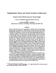
As one illustrative example, we present here the result of clustering the iris data (excluding, of course, the class attribute) with the Gustafson–Kessel algorithm using three cluster of fixed size (measured as the isotropic radius) of 0.4 (since all dimensions are normalized to mean 0 and standard deviation 1, 0.4 is a good size of a cluster if three clusters are to be found). The result without shape regularization is shown in Figure 1 on the left. Due to the few data points located in a thin diagonal cloud on the right border on the figure, the middle cluster is drawn into a very long ellipsoid. Although this shape minimizes the objective function, it may not be a desirable result, because the cluster structure is not compact enough. Using shape regularization method 2 with r = 4 the cluster structure shown on the right in Figure 1 is obtained. In this result the clusters are more compact and resemble the class structure of the data set. As another example let us consider the result of clustering the wine data with the fuzzy maximum likelihood estimation (FMLE) algorithm using three clusters of variable size. We used attributes 7, 10, and 13, which are the most informative w.r.t. the class assignments. One result without size regularization is shown in Figure 2 on the left. However, the algorithm is much too unstable to present a unique result. Often enough clustering fails completely, because one cluster collapses to a single data point—an effect that is due to the steepness of the Gaussian probability density function. This situation is considerably improved with size regularization, a result of which (which sometimes, with a fortunate initialization, can also be achieved without) is shown on the right in Figure 2. It was obtained with method 3 with r = 2. Although the result is still not

Fig. 2. Result of fuzzy maximum likelihood estimation (FMLE) algorithm on the wine data with fixed cluster weight without (left) and with size regularization (right, method 3 with r = 2). Both images show attribute 7 (horizontal) and attribute 10 (vertical). Clustering was done on attributes 7, 10, and 13. .

unique and sometimes clusters still focus on very few data points, the algorithm is considerably more stable and reasonable results are obtained much more often than without regularization. Hence we can conclude that size regularization considerably improves the robustness of the algorithm.

6

Conclusions

In this paper we suggested shape and size regularization methods for clustering algorithms that use a cluster-specific Mahalanobis distance to describe the shape and the size of a cluster. The basic idea is to introduce a tendency towards equal length of the major axes of the represented (hyper-)ellipsoid and towards equal cluster sizes. As the experiments show, these methods improve the robustness of the more sophisticated fuzzy clustering algorithms, which without them suffer from instabilities even on fairly simple data sets. Regularized clustering can even be used without an initialization by the fuzzy c-means algorithm. It should be noted that with a time-dependent shape regularization parameter one may obtain a soft transition from the fuzzy c-means algorithm (spherical clusters) to the Gustafson-Kessel algorithm (general ellipsoidal clusters). Software A free implementation of the described methods as command line programs for expectation maximization and fuzzy clustering can be found at http://fuzzy.cs.uni-magdeburg.de/~borgelt/software.html#cluster

References 1. J.C. Bezdek. Pattern Recognition with Fuzzy Objective Function Algorithms. Plenum Press, New York, NY, USA 1981 2. J.C. Bezdek, J. Keller, R. Krishnapuram, and N. Pal. Fuzzy Models and Algorithms for Pattern Recognition and Image Processing. Kluwer, Dordrecht, Netherlands 1999 3. J. Bilmes. A Gentle Tutorial on the EM Algorithm and Its Application to Parameter Estimation for Gaussian Mixture and Hidden Markov Models. University of Berkeley, Tech. Rep. ICSI-TR-97-021, 1997 4. C.L. Blake and C.J. Merz. UCI Repository of Machine Learning Databases. http://www.ics.uci.edu/~mlearn/MLRepository.html 5. H.H. Bock. Automatische Klassifikation. Vandenhoeck & Ruprecht, G¨ ottingen, Germany 1974 6. A.P. Dempster, N. Laird, and D. Rubin. Maximum Likelihood from Incomplete Data via the EM Algorithm. Journal of the Royal Statistical Society (Series B) 39:1–38. Blackwell, Oxford, United Kingdom 1977 7. R.O. Duda and P.E. Hart. Pattern Classification and Scene Analysis. J. Wiley & Sons, New York, NY, USA 1973 8. H. Engl, M. Hanke, and A. Neubauer. Regularization of Inverse Problems. Kluwer, Dordrecht, Netherlands 1996 9. B.S. Everitt and D.J. Hand. Finite Mixture Distributions. Chapman & Hall, London, UK 1981 10. I. Gath and A.B. Geva. Unsupervised Optimal Fuzzy Clustering. IEEE Trans. Pattern Analysis & Machine Intelligence 11:773–781. IEEE Press, Piscataway, NJ, USA, 1989 11. E.E. Gustafson and W.C. Kessel. Fuzzy Clustering with a Fuzzy Covariance Matrix. Proc. 18th IEEE Conference on Decision and Control (IEEE CDC, San Diego, CA), 761–766, IEEE Press, Piscataway, NJ, USA 1979 12. F. H¨ oppner, F. Klawonn, R. Kruse, and T. Runkler. Fuzzy Cluster Analysis. J. Wiley & Sons, Chichester, England 1999 13. A. Keller and F. Klawonn. Adaptation of Cluster Sizes in Objective Function Based Fuzzy Clustering. In: C.T. Leondes, ed. Database and Learning Systems IV, 181–199. CRC Press, Boca Raton, FL, USA 2003 14. F. Klawonn and R. Kruse. Constructing a Fuzzy Controller from Data. Fuzzy Sets and Systems 85:177-193. North-Holland, Amsterdam, Netherlands 1997 15. T. Kohonen. Learning Vector Quantization for Pattern Recognition. Technical Report TKK-F-A601. Helsinki University of Technology, Finland 1986 16. T. Kohonen. Self-Organizing Maps. Springer-Verlag, Heidelberg, Germany 1995 (3rd ext. edition 2001) 17. R. Krishnapuram and J. Keller. A Possibilistic Approach to Clustering, IEEE Transactions on Fuzzy Systems, 1:98-110. IEEE Press, Piscataway, NJ, USA 1993 18. A.N. Tikhonov and V.Y. Arsenin. Solutions of Ill-Posed Problems. J. Wiley & Sons, New York, NY, USA 1977 19. H. Timm, C. Borgelt, and R. Kruse. A Modification to Improve Possibilistic Cluster Analysis. Proc. IEEE Int. Conf. on Fuzzy Systems (FUZZ-IEEE 2002, Honolulu, Hawaii). IEEE Press, Piscataway, NJ, USA 2002