Jan 5, 2005 - ... in digital form and processed in CAD/CAM/CAE, entertainment, ... may capture the interplay between solids and lower dimensional elements.
January 5, 2005
Shape Complexity Jarek Rossignac College of Computing, GVU Center, and IRIS cluster Georgia Institute of Technology, Atlanta, Georgia http://www.gvu.gatech.edu/~jarek/
Abstract The complexity of 3D shapes that are represented in digital form and processed in CAD/CAM/CAE, entertainment, biomedical, and other applications has increased considerably. Much research was focused on coping with or on reducing shape complexity. But, what exactly is shape complexity? We discuss several complexity measures and the corresponding complexity reduction techniques. Algebraic complexity measures the degree of polynomials needed to represent the shape exactly in its implicit or parametric form. Topological complexity measures the number of handles and components or the existence of non-manifold singularities, non-regularized components, holes or selfintersections. Morphological complexity measures smoothness and feature size. Combinatorial complexity measures the vertex count in polygonal meshes. Representational complexity measures the footprint and ease-of-use of a data structure, or the storage size of a compressed model. The latter three vary as a function of accuracy.
1. Introduction Digital models of 3D shapes are common in numerous applications. They are used to represents solids, which correspond to physical objects, surfaces, which may—but need not—bound a solid, or more general geometric complexes, which may capture the interplay between solids and lower dimensional elements. So far, the accuracy of models that could be represented in 3D modeling systems has been limited by design or acquisition costs, by storage and transmission costs, by computational and visualization costs, and also by theoretical and implementation challenges. These costs are directly related to the complexity of a shape or of the representation used to store it in digital form. A large body of research has been focused on reducing these costs. Computational Geometry techniques [GoOR04] play an important role in reducing the asymptotic time or space cost of algorithms that construct or process polygonal representations of 3D shapes. They will not be discussed explicitly here. Instead, we investigate the following complementary aspects. In Section 2, we briefly discuss the complexity stemming from the use of higher order polynomials to represent the surfaces that bound a shape. In Section 3, we review the broad topological domain of shapes and structures that can be represented as a Selective Geometric Complex and discuss how to map this domain to solids or even manifolds, and how to reduce their genus. Complexity may be measured in terms of sharp or narrow features, hence, in Section 4, we discuss the smoothness and regularity of shapes, and techniques for increasing them. In Section 5, we discuss lossy simplification and retiling techniques for shapes represented as triangle meshes. In Section 6, we discuss simple and compact data structures for CSG and BRep and provide examples of redundancy reduction and compression schemes. Due to space limitations, we do not discuss design complexity, nor visual complexity.
2. Algebraic complexity Digital representations of solid objects [OKK73, Mant88] are often defined by arranging simpler shapes and by combining them through Boolean operations. In particular, a solid may be specified in Constructive Solid Geometry (CSG) as a Boolean combination [Mant86] of primitive solids whose dimensions, position, and orientation may be conveniently controlled by the user [ERR93]. A primitive solid may be easily defined in its nominal position and orientation as the set of points, whose coordinates satisfy one or several polynomial inequalities. For example, a ball of radius r is the set of points (x,y,z) satisfying x2+y2+z2≤r2. The complexity of such a semi-algebraic representation of a solid may be measured by the number of primitives (discussed in Section 6) or by the degree of the polynomials used to represent them. Early CSG modelers were limited to linear polynomials [BrEv85], approximating curved primitives by facetted models that could be represented as intersections of linear inequalities or as extrusions of polygonal contours. In the 70s and 80s, commercial products provided support for a subset of quadric primitives [BRV78]. More recently, techniques for rendering Boolean combinations of more general surfaces have been demonstrated [BKZ01] and more complex analytic formulations were proposed to extend the Booleans operations [PASS95]. Semi-algebraic formulations are implicit and make it difficult to answer simple geometric or topological queries. For example, a solid represented by a CSG model with an arbitrarily large number of primitives could actually be empty. Furthermore, popular rendering and analysis systems are geared towards boundary representations (BReps), where each face of the solid is represented as a node in a global incidence graph. A face is a two-dimensional portion of a surface and hence is also called a trimmed surface [SPPK04]. Surfaces of CSG primitives are defined in terms of polynomials. For
example, the surface may be defined by an implicit polynomial equation, such as the equation x2+y2+z2=r2 of a sphere. The face may be specified as the intersection of the surface with a trimming volume. Such a trimming volume may be represented in semi-algebraic (CSG) form, which may be readily extracted from the original CSG formulation of the solid [Ross96]. But such an implicit representation of the trimming volume still suffers from the same limitations as the CSG representation: It does not tell us explicitly whether the face exists, whether it is connected, or whether it has holes. To capture this topological information, an explicit boundary representation of a trimmed surface is usually computed through Boundary Evaluation [ReVo85]. The explicit representation of a face consists of the implicit (polynomial) equation of the supporting surface and of a representation of the bounding edges that delimit the face. These edges are usually portions of curves, where two implicit surfaces intersect. A parametric representation C(s) of each intersection curve is preferred. It may be derived in closed form for various combinations of simple quadric surfaces [MiGo95]. The vertices, where bounding edges meet may be computed by substituting the coordinate functions of C(s) in the implicit equation of a third surface and solving for s. This approach has been principally limited to quadric surfaces for which intersection vertices may be computed by finding the roots of low degree polynomials. More complex (i.e. higher order) primitives yield systems of simultaneous polynomial equations of higher order, raising the complexity of a robust rootfinder and the computational cost of the boundary evaluation [LPP04]. Hence, the term CSG usually refers to systems that support Boolean combinations of primitive solids bounded by linear or specific quadric polynomials. Although any solid may be approximated by a CSG model, a close approximation of a sculptured (free-form) shape [Ll&00] may require a large number of quadric primitives. The alternative is to use a parametric formulation, where each face is still represented as a trimmed surface, but the supporting surface is a mapping, M, of a unit square (u,v)∈[0,1]2 in parameter space onto a set of 3D points M(u,v) and where the bounding edges are represented as parametric trimming curves (u(s),v(s)) in the two-dimensional parameter space. A parametric curve is the set of points (u(s),v(s)), where u and v are piecewise polynomial or rational polynomial functions in s [FHK02]. Typically, these are polynomials of degree 3 or less, although aesthetic or functional constraints may require higher order polynomials. In this parametric trimmed surface representation, each trimming edge is represented twice (once for each incident face). When the edge is computed as the intersection between two faces during a Boolean operation, the two representations may not match, creating a gap or selfintersection in the boundary. Such inconsistencies may undermine the integrity of subsequent algorithmic computations. This inconsistency problem, as well as the problem of detecting and tracing intersections of parametric surfaces [KPW92], is exacerbated if higher order parametric surfaces or trimming curves are used. The immense software complexity of several commercial CAD systems [Korm85] is in a large part due to the difficulty of performing and processing reliably the intersections of parametric surfaces. Hence some 3D modelers require that the user designs the boundary of a solid as a patchwork of abutting untrimmed parametric patches, thus significantly increasing the complexity of the design process. To avoid dealing with higher-order parametric formulations, one may choose to use only first degree polynomials, for which the CSG-to-Boundary conversion may be performed reliably [BaRo96]. With such a choice, all surfaces are planes and all edges are line segments. Such polygonal models are popular in graphics and animation, because the software for computing and representing them is less complex and because hardware accelerators have been optimized for rendering them. However, a close approximation of a curved shape may require a large number of planar facets, increasing its combinatorial complexity, storage size, transmission time, processing costs, and rendering delays. Finally, note that BRep modelers are not restricted to solids and can also be used to model surfaces that do not bound a solid and more general geometric complexes, as discussed in the next section. In summary, the designer of a 3D modeler that supports Boolean operations must chose between a CSG (implicit) or a BRep (parametric) scheme and decide on the degree of polynomial surfaces supported. The choice will impact the complexity of the software and also the growth of the combinatorial complexity as a function of the accuracy with which a particular shape is approximated.
3. Topological complexity Although the representation of solids [Requ80] has always been a major focus of CAD and animation systems, it is often desired or even necessary to represents 3D geometries that are not solids, nor even boundaries of solids. Such geometries may arise in reverse engineering, where surface samples are erroneously interpolated by a surface that does not constitute the boundary of a solid; in analysis, where it may be important to represent the contacts between solids; or during the design of mixed-dimensional structures combining inhomogeneous solids with lower-dimensional elements. The concept of a Selective Geometric Complex [RoOC89] was developed to provide a common theoretical framework for representing solids, lower-dimensional elements (points, curves, surfaces) and their interactions. To discuss its topological complexity and the corresponding simplification operations, we consider that a pointset S decomposes space into 6 subsets [Ross04b]: iS, eS, sS, wS, cS, and hS. To define them, let ~S denote the complement of S. Let Br(p) be an open ball of radius r around a point p. Let b(s), denoted bS for simplicity, be the boundary of S. It is defined as the set of points p for
J. Rossignac
Shape Complexity
2 / 12
which Br(p) intersects both S and ~S for all strictly positive r. The interior iS is S–bS. The exterior eS is (~S)–bS. The skin sS is the portion (biS)∩(~S) of bS that is included in S and is separating S from ~S. The wound wS is the portion (beS)∩(~S) of bS that is not included in S and separates S from ~S. The hair hS is the set (beS)∩S of dangling faces, edges, and isolated vertices of bS included in S that are not bounding iS. The cut cS is the union of the cracks (biS)∩(~S) that are not part of S, but are not bounding eS. A set S is open if S=iS, i.e. it has no skin or hair. A set is closed if it has no wound or cut. The closure, kS, of a set S is (iS)∪(bS). A set S is regularized, when it has no wound, no hair, and no cut. To convert an arbitrary set S into a regularized (“clean”) set, we need to “cut its hair, mend its cut, and grow back the skin over its wound”. The regularized version rS of S may be formally defined by (iS)∪(cS)∪(sS)∪(wS) or more compactly as kiS. Hence, S is regularized if S=kiS. The effect of these various topological operators is shown in Fig. 1.
S Skin
Exterior
Wound iS
Interior
Hair
iS
bS bS
kS
kS
Cut
Figure 1: The interior, exterior, and the four boundary types are shown (left). The effects of the interior, boundary, and closure operators are shown on a non-regularized set (right).
The Selective Geometric Complex (SGC) representation [RoOC89, Ross97] was designed as an extension of the Boundary Representation (BRep) to the broader domain of non-regularized pointsets. In an SGC, each cell (volume, face, edge) knows the extent (the whole space, an implicit algebraic surface, a parametric or implicit curve) in which it is embedded, the list of its bounding elements, and its membership (a bit indicating whether it is part of S or of ~S). Hence, marking a face as part of ~S may create a wound (if it is adjacent to both iS and eS) or a cut (if it is surrounded by iS). Furthermore, with the reference to each (k–1)-dimensional bounding element e of a k-dimensional set f, is associated a two-bit neighborhood indicating whether e is bounding f on its left, on its right, or on both sides. The terms left and right are defined with respect to an agreed-upon orientation of e and f. This neighborhood information permits, for example, to specify a particular half-sphere as a subset of a spherical extent bounded by a single circle. Given the orientation of the sphere and of the circle, the neighborhood indicates which half of the sphere is of interest. The broad topological domain of SGCs may be appropriate for annotating models with internal structures, for representing shapes with cracks, for modeling boundary conditions, or for representing a regularized model during intermediate stages of its construction. Unfortunately, the support of non-regularized shapes adds complexity to a modeling software. For instance, to decide whether a point p not on bS lies inside a solid S, one would usually cast an arbitrary ray from p making sure that the ray does not hit any edge or vertex of bS and does not have a tangential intersection with bS. Then, one would compute the parity of the number of times the ray crosses bS [Tilo80]. An even number of intersections indicates that p is out of S, because a point infinitely far along the ray is out of S (assuming that S has finite size). If S is not regularized, the test must be modified to discard intersections with hair and cut faces. Hence, a BRep of S must explicitly distinguish between the skin, wound, hair, and cut portions of bS. Although such a distinction is provided by the SGC representation scheme [RoOC89], early solid modelers, were limited to solids (regularized sets). Because Boolean intersection and difference operations between two regularized sets with partly overlapping boundaries may produce non-regularized sets [RoRe91], these modelers automatically performed a regularization of the resulting sets (eliminating cut, hair, and wounds), ensuring that all nodes in the CSG tree represent solids. This regularization, i.e., the extraction of the regularized version kiS of a non-regularized model S, may be viewed as a reduction in topological complexity. In an SGC representation, this regularization operation amounts to setting the membership bit to IN for all cut and wound cells and to OUT for all hair cells. The removal of the redundancy in the resulting SGC representation is discussed in Section 6. Assume that the we are given a set B, which approximates the valid boundary bS of a solid S, but contains inconsistencies (gaps between adjacent faces, self intersections), which may have resulted from an inaccurate reverse engineering process or from inconsistencies between the two representations of each trimming edge in a parametric model, as discussed in the
J. Rossignac
Shape Complexity
3 / 12
previous section. The extraction of bS from B is sometimes called healing or repairing. It is a difficult process, since B does not unambiguously define S. When B is a set of faces defined as trimmed portion of oriented implicit surfaces, their extents partition the space into an arrangement of three-dimensional cells. S may be estimated [MuTh97] by a voting scheme, in which the larger cells of the arrangement that are bounded by large portions of faces of B are given a higher probability of being in S (if they lie on the interior side of the oriented face) or in ~S (otherwise). Some scanned models are incomplete. The missing parts of their boundary are called holes. The process of filling the holes in such models [Liep03] is different from the healing discussed above, because the holes are typically larger than the gaps in an inconsistent BRep. These incomplete models may be produced by the early stages of a reverse engineering process, which starts with a set P of discrete points sampled on bS. The process of recovering bS from P is sometimes called point cloud interpolation. Several approaches have recently been proposed for this difficult task [TaDe04]. Healing, hole filling, and point cloud interpolation may be viewed as a reduction of the topological complexity of the representation of a regularized shape S, because they simplify further processing, although one could argue that P is topologically simpler than S or bS. In fact, several researchers are exploring the use of point clouds for modeling and rendering 3D shapes [PZBG00]. Through the remainder of this paper, we will assume that S is a solid (finite regularized set). Note that a solid may be manifold or not. A point p of bS is said to be manifold (with respect to bS) [Alex61] if there exists a positive r such that the intersection of bS with the open ball Br(p) is homeomorphic to an open disk. Otherwise, p is said to be non-manifold. S is manifold if all points of bS are manifold. Consider a non-manifold solid S. Let N denote the set of its non-manifold points. In turn, N may be decomposed [RoOC89] into a set of relatively open curves, which we call the non-manifold edges (NME), and a set of isolated points, which we call non-manifold vertices (NMV). Support of non-manifold situations complicates algorithms for processing S or for performing Boolean operations between sets. Yet, non-manifold singularities cannot be easily avoided, since they are produced by Boolean operations on solids in tangential contact. When a NME has k pairs of incident faces, it may be replaced by k coincident manifold edge-instances, each having one pair of incident faces. Several choices of pairing the incident faces are possible. Amongst those, one should match faces that have a compatible orientation so that there exists a way of bending each one of the k manifold edge-instances into a different curved edge so that the resulting BRep is free from self-intersection [RoCa99]. At the end of this process all edges are manifold, although clusters of edge-instances may be geometrically coincident. The model may still be non-manifold, because it may have non-manifold vertices. These are vertices with two or more cycles (fans) of incident faces. A NMV with k cycles is replaced by k coincident vertex-instances. The resulting model has a manifold topology that is inconsistent with its imbedding in space. Hence, it can be represented by a data structure designed for manifold solids, although the algorithms that process it may no-longer assume that all pairs of edges and of vertices are mutually disjoint. Techniques for converting non-manifold models to such pseudo-manifolds in a manner that minimizes the number of vertex-instances have been proposed [RoCa99]. We assume hereafter on that the solids are either manifold or pseudo-manifolds. A solid may have more than one connected component. Furthermore, each component may be bounded by one or more shells (connected portions of the boundary). Finally, each shell may have one or more handles. The number of handles is called the genus of the shell. The genus affects the programming complexity of various algorithms and the efficiency (representational complexity) of some encodings [Ross99]. Hence, it may be desired to compute approximations of a solid S that have lower genus, or that are simply connected (bounded by a single, genus-one shell). Genus reduction may be achieved [SzVa03] by starting with a simply connected boundary of a solid that contains S and shrinking the boundary while preventing changes of genus and intersections with S. A distance field may be used to control the shrinking speed. By identifying and allowing a few initial changes of topology, a desired number of the larger handles may be created, removing the smaller ones. Similarly, one may wish to remove small shells. These are easy to identify, since one may quickly compute an axis aligned minimum bounding box containing each component. Hence, one may construct decreasingly complex approximations of S, where the number of handles and/or components is decreasing. Such an approach may be viewed as a filter that eliminates topological noise, possibly produced through a point-cloud interpolation of an insufficiently dense set of points produced by a 3D scan of a real shape. Consider now that B is an isosurface separating all points on a regular 3D grid where some measure (say pressure) is higher than a threshold from those where the measure is lower. The topology of B is not fully defined. Local topology choices and simple optimizations [An&04] may be used to reduce the number of handles or shells, while reducing the representational complexity (vertex count) of the isosurface. In summary, although it is possible and sometimes essential to support non-regularized shapes, many applications are not designed to cope with such topological complexity. Hence, such representations must often be converted to solids through regularization. Furthermore, non-manifold edges and vertices may be replaced by multiple instances of their manifold counterparts. Finally, the boundary of a solid may be replaced by an approximating surface that exhibits fewer handles and shells. The designer of a modeling system must decide which level of topological complexity will be supported and may provide simplification techniques that reduce the complexity of a particular model.
J. Rossignac
Shape Complexity
4 / 12
4. Morphological complexity Shape having more numerous or smaller features may be viewed as more complex. To evaluate and reduce this morphological complexity, one needs to define what a feature is, measure its size, and provide algorithms for computing an approximation of a shape, where the identified features are larger or fewer. We may distinguish [WiRo05] two measures of morphological complexity: Smoothness and Regularity. If a point p of bS is non-manifold or if the maximum curvature of bS at p is not well defined, we say that the smoothness of p (with respect to S) is zero, or equivalently that p is zero-smooth. Otherwise, we define the smoothness of p as the inverse, 1/c(p), of the maximum curvature [Taub95] of bS at p. The smoothness of S is the minimum of the smoothness of points on bS. For instance, if S has a sharp edge, its smoothness is 0. We say that solid S is r-smooth if its smoothness is equal to or larger than r. At each point p of bS, one may also compute the maximum radius r(p) of an open ball that can touch p from both sides of bS without intersecting bS. The regularity of S is the minimum of r(p) over all points p of bS. A shape is r-regular if its regularity is equal to or larger than r. Note that if S is r-regular, then it is r-smooth. However, a shape may be r-smooth, but may contain small constrictions or cracks that are not r-regular. The regularity of a point of bS is its local feature size, which is its distance to the medial axis of bS. The medial axis is the set of points having more than one closest point on bS. Hence, the regularity of bS is its least feature size. The definition proposed in [WiRo05] extends the notion of regularity to the whole space: the regularity of a point p in iS or eS is the radius of the maximum open ball Br(p) that contains p and is disjoint from bS. To reduce the morphological complexity of a shape, one may increase its smoothness or its regularity. When bS is a triangle mesh, its smoothness may be increased through subdivision [Loop94, DLG90, WaHa02] or through smoothing [Taub95b]. Subdivision replaces a triangle mesh with a finer mesh. Iterating the process converges to a smooth surface [ZSS96]. Subdivision splits each triangle into smaller triangles by introducing new vertices and possibly adjusting the old ones. The limit surface tends to be smoother everywhere, unless it contains non-manifold singularities or self-intersections produced during subdivision. Smoothing alternates moving each vertex towards the average of its neighbors and moving it away from this average. Moving towards the neighbors smoothens the shape. Moving away prevents shrinkage [Taub95b]. Since smoothing does not increase the number of vertices, the resulting mesh has zero smoothness at all non-flat edges and vertices and hence is zero-smooth and zero-regular. However, smoothing reduces discrete measures of curvature estimated at the vertices [Taub95], at least away from thin tubes (see Fig 2). Shapes may also be smoothened through curvature flow, which may be implemented using level sets [Seth99].
Figure 2: The original solid bounded by a triangle mesh (left) has been smoothened (right). Note that the resulting shapes need no longer regularized, because smoothing has squeezed thin parts into lower-dimensional dangling edges or produce self-intersections.
Because the subdivision and smoothing techniques discussed above do not provide a direct control over the desired degree of smoothness or regularity, morphological filters may be preferred when more control on smoothness and regularization is desired The r-rounding Rr(S) of S is the union of all balls of radius r contained in S. The r-filleting Fr(S) is the pointset that cannot be reached by a ball of radius r disjoint from S. Note that Fr(Rr(S)) and Rr(Fr(S)) [Ross85] leave the r-regular portions of bS unchanged and tend to produce shapes that are almost everywhere r-smooth and r-regular. More precisely, they modify bS only in the r-mortar Mr(S), defined as Fr(S)–Rr(S) [WiRo05]. However, Fr(Rr(S)) tends to shrink the solid and Rr(Fr(S)) tends to grow it. To alleviate this bias, the Mason filter [WiRo05] identifies the connected components of Mr(S) and includes in the result only the components that have more than 50% of their volume in S (Fig. 3). Instead of this binary decision, the Tightening [WiRo04] filter tightens bS inside the r-mortar. The tightening process may change the topology of bS and guarantees that the boundary of the r-tightening Tr(S) of S is r-smooth everywhere. Although there is
J. Rossignac
Shape Complexity
5 / 12
no guarantee that Tr(S) is r-regular, the irregular singularities are rare and tend to be isolated. Finally, the boundary of Tr(S) is obtained by minimizing surface area.
Figure 3: The morphological complexity of the original solid (left) has been reduced (right) by using the Mason filter.
The geometric error (discrepancy) between S and its morphological simplification S’, which may be Fr(Rr(S)), Rr(Fr(S)), r-Mason(S), or Tr(S), is bounded in the following way. Every point of bS’ lies within a tolerance zone Zr(bS) of all points within distance r from bS. However, the reverse is not true and there usually are points of bS that lie further than r from bS’. For instance, whole shells of bS may be removed through morphological simplification. Nevertheless, note that these simplifications confine their effect to the r-mortar Mr(S), which is usually a very small subset of Zr(bS). In summary, one may measure the morphological complexity of a solid S as the largest value of r for which S is r-regular or simply r-smooth. Complexity measured in terms of smoothness may be reduced indirectly through subdivision or smoothing. When a more precise control is needed, morphological filters may be used. In particular, the r-tightening guarantees to produce a shape that is r-smooth and has minimal area boundary. In general, the resulting shape is also rregular almost everywhere.
5. Combinatorial complexity In many applications, piecewise planar boundaries are preferred to higher degree polynomial surfaces. The boundary bS of a solid S is usually represented by a set of surface samples (called vertices) and by a connectivity graph defining a triangle mesh that interpolates the vertices and approximates the desired surface. (Although many modelers support more general polygonal faces, these may always be each represented as a set of contiguous triangles. If desired, one bit per edge may be stored to distinguish between the original edges and those introduced through this artificial triangulation. This conversion to triangle meshes leads to significantly simpler algorithms and to more compact and more regular data structures.) The complexity of a triangle mesh may be simply formulated as its vertex-count. Because vertex-count impacts storage size, algorithmic complexity, and rendering performance, various simplification techniques have been proposed for reducing the vertex-count. When an edge of the triangle mesh is collapsed, its two bounding vertices are clustered into one and its two incident triangles may be removed. Hence, each edge-collapse operation [Ho&93] reduces the vertex count by 1 and the triangle count by 2. Most triangle mesh simplifications operate by performing a series of edge-collapses. For each edge collapse, two vertex-clusters are merged, the cluster-representative vertex position is computed (maybe as the one that minimizes some error estimate), and the resulting error is recorded. A priority queue may be maintained to accelerate the selection of the edge-collapse that will result in the lowest error. At each stage, the edge with the smallest error is collapsed and the vertex representatives and cost of collapsing neighboring edges updated. The process stops when the desired reduction of vertex-count has been achieved or when the error estimate exceeds a prescribed tolerance. The various approaches differ in their strategy for selecting which edge to collapse next and where to position the new cluster-representative vertex. The error between the original surface S and the surface S’ produced by one or more edge-collapses may be measured in different ways. Computing the Hausdorff error H(S,S’), which is defined as the minimum r such that bS’⊂Zr(bS) and bS⊂Zr(bS’) is difficult and expensive [CRS98, Ross04b]. Hence, simpler bounds or estimates of H(S,S’) are usually used. Ronfard and Rossignac [RoRo96] have used, as vertex-representative of a cluster, the point that minimizes the sum of the squares of the distances to the extents (supporting planes) of each triangle incident upon a vertex of the cluster. To estimate the error, they used the maximum of the squares of the distances to the extents. This solution required merging lists of extents as the clusters were merged, but provided a conservative bound on the Hausdorff error. Garland and Heckbert [GaHe97] have replaced the maximum by the sum of the squares of the distances to the extents. This is called the
J. Rossignac
Shape Complexity
6 / 12
quadratic error. As a result, they needed only to keep track of the 10 coefficients of a quadratic polynomial in the coordinates of the vertex representative. When two clusters are merged, the coefficients of the quadratic error of the new cluster may be obtained by simply adding their counterparts in the quadric error formulation of each cluster. This simplification of the simplification process has led to a very efficient and effective combinatorial complexity reduction technique [Garl99], at the cost of replacing the maximum error by the L2 error measure. Triangle mesh simplifications based on edge-collapses do not alter the topology of the shape, unless, they unintentionally produce self-intersecting boundaries. Although topology preservation may be required in some applications, it considerably limits the level of reduction in the vertex-count that may be achieved for a given tolerance (error). Furthermore, edgecollapsing is usually implemented for manifold boundaries of regularized solids. In contrast, the Vertex-clustering method [RoBo93] works well on non-regularized shapes, which may combine non-manifold solids with lower dimensional construction lines, 2D drawings, and even annotations. It tends to merge small components, remove small holes, and reduce thin sheets or tubes to their lower-dimensional approximations of the medial axes or skeletons (Fig. 4). Vertexclustering makes clusters of vertices that fall within the same cell of a three-dimensional regular grid. Consequently, it is extremely fast and simple to implement. The Hausdorff error H(S,S’) and the length of collapsed edges are bounded by the length of the diagonal of a cell. Hence, vertex-clustering is less effective at reducing the vertex count than edge-collapsing in over-tessellated flat regions. Therefore, several authors have proposed to combine both approaches [Lu&02].
Figure 4: The combinatorial complexity of an assembly with its drawing (left) has been reduced (right) through vertex clustering.
In summary, the reduction of combinatorial complexity is a lossy process, trading accuracy for simplicity. Most of the research in this area has been focused on reducing the vertex-count of triangle meshes [Lu&02]. Several efficient simplification techniques exist and may be combined to simplify smooth manifold surfaces effectively, to allow topological changes that further reduce vertex-count, and to operate on non-regularized models.
6. Representational complexity The reduction of combinatorial complexity, as discussed above, is accompanied by a loss of accuracy. In contrast, the techniques for reducing the representational complexity, discussed in this section are loss-less. We discuss techniques for removing the redundancy in SGC representations, in CSG representations, and in triangle mesh representations. We also discuss compact loss-less encodings (compression) of the connectivity of triangle meshes and how they are affected by a lossy re-sampling preprocessing step. As mentioned in Section 3, the topological complexity of the SGC representation of a non-regularized model may have been reduced by changing the membership bits of specific cells, for instance to eliminate the wound, the cut, or the hair of a model during a closure, interior, or regularization operation. As a result, some of the lower-dimensional cells may be eliminated or merged with incident higher-dimensional cells in order to reduce the representational complexity of the model stored in SGC form. For example, a dangling edge or face of the hair marked OUT may be dropped, a face marked IN and its two incident three-dimensional cells of iS may be joined, or an edge originally part of cS, but marked IN, may be merged with its only incident face of iS. The preconditions and algorithms for these drop, join, and merge operations that ensure the validity of the resulting SGC are discussed in [RoOC89]. The representational complexity of a solid stored in CSG form may sometimes be reduced by discovering that the same solid may be represented with fewer CSG primitives. A primitive may be eliminated if it is redundant [Tilo84]. Consider a primitive A in the CSG representation of a solid S. We can write S as a set-valued function S(A) of A. The active zone [RoVo89] Z of A in the CSG expression of S is defined as S(W)–S(E), where W is the universe and E the empty set. If A is disjoint from Z, then A is E-redundant and can be replaced by the empty set. If A contains Z, then it is W-redundant and may be replaced by W. Replacing A by E or W yields a simplification of the CSG expression, by the successive application
J. Rossignac
Shape Complexity
7 / 12
of simple re-write rules, such as W∪B=W, W∩B=B, E∪B=B, and E∩B=E, using the fact that B–C=B∩(~C) and that ~(B∪C)=(~B)∩(~C) and ~(B∩C)=(~B)∪(~C). Redundancy detection, which requires testing whether A∩Z or A–Z are empty may be accelerated by using s-bounds [RoCa88], which are computed. The representational complexity of a solid whose boundary is stored as a triangle mesh may be measured by storage size or by the complexity of the underlying data structure and of the associated algorithms. Consider a triangle mesh defined by its geometry and by its triangle-vertex incidence graph. The geometry is stored as an array of vertex-entries (3 coordinates per vertex). Incidence (sometimes called “topology”, referencing the connectivity graph) defines each triangle by listing the 3 integer indices that identify its vertices. Consider a triangle mesh with v vertices, e edges, and f triangular faces. To simplify some of the definitions, we assume that the faces and edges are relatively open cells, i.e., they do not contain their boundary in the supporting manifold [RoOC89]. We say that the mesh is edge-connected if all pairs of triangles form the two ends of some strip of triangles in the mesh. A strip is an ordered list of triangles such that two consecutive elements of the strip are incident upon a common edge. A Vertex-Spanning Tree (VST) of a triangle mesh is a subset of the edges of the mesh, selected so that their union with all the vertices forms a tree (connected cycle-free graph). Consider that a given VST has been selected. The edges it contains are called the cut-edges. The union of the cut-edges with all the vertices is called a cut (not to be confused with the topological cut defined in Section 4). Because the VST is a tree, there are v–1 cut-edges. The difference between the surface and its cut is called the web. Edges that are not cut-edges are called hinge-edges. The web is the union of the faces and hinge-edges. Removing the cut, which has no loop, from the surface of a mesh will not disconnect it. Assume first that the mesh forms a surface that is homeomorphic to a sphere. The removal of the cut produces a web that is a (relatively open) triangulated two-dimensional point-set in three-space. This web is simply connected and may be represented by an acyclic graph, whose nodes correspond to faces and whose links correspond to hinge edges. The web forms a planar triangulation and can be drawn on the plane so that no two faces overlap. Thus there are f–1 hinge edges. Note that by picking a leaf of this graph as root and orienting the links, we can always turn it into a binary tree, which we call the Triangle-Spanning-Tree (TST). The TST defines a connected network of corridors (strips) through which one may visit all the faces by walking across hinge-edges and never crossing a cut-edge. Because an edge is either hinge or cut, the total number of edges, e, is v–1+f–1. Each face uses 3 edges and each edge is used by 2 faces. Thus, the number e of edges is also equal to 3f/2. Combining these two equations yields f=2v–4, which shows that there are roughly twice as many triangles as vertices. When the mesh forms a manifold surface of genus h, this equation becomes f=2v+4h–4 and the web is no longer simply connected, but has 2h handles. It can be flattened (i.e. turned into a simply connected open polygon) by removing 2h additional edges, which we call the jump edges [TaRo98]. More generally, the mesh may also have holes and non-manifold singularities, which further complicates the relation between f and v. Although a large number of representation schemes have been proposed for triangle meshes [Ross94] and more generally for polygonal meshes, we advocate the use of a Corner Table [RSS01, RSS03] because of its simplicity. The Corner Table stores the geometry in the G table and the connectivity in the V and O tables of integers, each having 3f entries. Each entry G[v] contains the triplet of the coordinates of vertex number v, and will be denoted v.g. Note that the order in which the vertices are listed in G is arbitrary, although once chosen, it defines the integer reference number associated with each vertex. Triangle-vertex incidence defines each triangle by the three integer references to its vertices. These references are stored as consecutive integer entries in the V table. Note that each one of the 3f entries in V represents a corner (association of a face with one of its vertices). Let c be such a corner. Let c.f denote its face and c.v its vertex. Remember that c.v and c.f are integers in [0,v–1] and [0,f–1] respectively. Let c.p and c.n refer to the previous and next corner in the cyclic order of vertices around c.f. Although G and V suffice to completely specify the faces and thus the surface they represent, they do not offer direct access to a neighboring face or vertex. We chose to use the reference to the opposite corner, c.o, which we cache in the O table to accelerate mesh traversal from one face to its neighbors. For convenience, we also introduce the operators c.l and c.r, which return the left and right neighbors of corner c (Fig. 5). Note that we do not need to cache c.f, c.n, c.p, c.l, or c.r, because they may be quickly evaluated as follows: c.f is the integer division c.f DIV 3; c.n is c–2, when c MOD 3 is 2, and c+1 otherwise; and c.p is c.n.n; c.l is c.n.o; and c.r is c.p.o. Thus, the storage of the connectivity is reduced to the O and V arrays. We assume that all faces have been consistently oriented, so that c.n.v=c.o.p.v for all corners c. For example, one may adhere to the convention that when a face c.f is visible by a viewer outside of the solid (i.e., the finite set that is bounded by the tri mesh), the three vertices, c.p.v, c.v, and c.n.v, appear in counter-clockwise order. The simplicity of the Corner Table data structure and the notation defined above simplify many of the algorithms that traverse, process, or modify the mesh. For example, the procedure visit(c) {if NOT c.f.m then {c.f.m:=true; visit(c.r); visit(c.l)}} will visit all the faces in a depth-first order of a TST, assuming that c.f.m is a Boolean set to true when the face c.f has been visited.
J. Rossignac
Shape Complexity
8 / 12
c.v
c.l
c.r
c
c.n
c.f c.p c.o
Figure 5: Corner operators for traversing a corner table representation of a tri mesh.
Given the V table, the entries in O may be computed by: for c:=0 to 3f–2 do for b:=c+1 to 3f–1 do if (c.n.v==b.p.v)&&(c.p.v==b.n.v) then {c.o:=b; b.o:=c}. A faster approach is described in [Ross04]. Because it can be easily recreated, the O table needs not be transmitted. Furthermore, the 31–log2v leading zeros of each entry in the V table need not be transmitted. Thus, assuming that Floats are used for the coordinates, a compact, but uncompressed representation of a triangle mesh requires 48f bits for the coordinates and 3flog2v bits for the V table. The Edgebreaker compression [Ross99] encodes the full connectivity information contained in both V and O with a linear cost of less than 2f bits, and hence eliminates the need for the decompression modules on the client to re-compute O from V. Edgebreaker performs a walk on a manifold surface which follows a breadth-first TST that is similar to the visit(c) procedure described above, but avoids the recursive call in most cases by using a bit-mask to mark all previously visited faces. Edgebreaker encodes one symbol out of the set {C,L,E,R,S} per triangle in the order in which the triangles are visited. Furthermore, because half of the symbols are a C, the string of symbols (also called the clers string) may be trivially encoded using 2f bits plus a small overhead per handle. Further reductions of this storage cost [KiRo99, RoSz99, SKR00, CoRo04] have been proposed, achieving a guarantee of 1.80f bits and often an entropy of less than 1.0f bits. When the connectivity of a triangle mesh is compressed as discussed above, the bulk of the storage cost is used to encode the location of the vertices (geometry). This cost may be reduced through geometry compression, which combines: a lossy quantization with loss-less prediction and statistical coding of the residues. Quantization truncates the vertex coordinates to a desired accuracy and maps them into integers that can be represented with a limited number of bits. Using 12 bit integers for each coordinate ensures a sufficient geometric fidelity for most applications. Both the encoder and the decoder use the same predictor to guess the location of the next vertex. The most popular parallelogram predictor [ToGo98] predicting c.o.v.g as c.n.v.g+c.p.v.g–c.v.g. The residues between the predicted and the correct coordinates are small integers, suitable for statistical compression [Salo00]. The combination of these three steps compresses vertex location data to about 7f bits. When there is no need to preserve the original connectivity or the original vertex locations, superior compression may be achieving by retiling the surface [Turk92]. Three different retiling approaches have been designed to increase compression. The Piecewise Regular Mesh (PRM) retiling approach [SRK02] decomposes the surface into 3 reliefs, each one comprising triangles whose normals are closest to one of the three principal directions. Each relief is resampled along a regular grid and the global connectivity of the new triangle mesh is recomputed. When the sampling rate is chosen so that the resulting PRM has roughly the same number of vertices as the original mesh the mean square error of less than 0.02% of the diameter of the bounding box. Because of the regularity of the sampling in each relief, the PRM may be compressed using a modified Edgebreaker down to a total about 2t bits, which accounts for both connectivity and geometry. SwingWrapper [Atte01], another retiling approach, partitions the surface of an original mesh M into simply connected regions, called triangloids. From these, it generates a new mesh M’. Each triangle of M’ is a linear approximation of a triangloid of M. By construction, the connectivity of M’ is regular (on average, 96% of the triangles are of type C or R, 82% of the vertices have valence 6) and can be compressed to less than a bit per triangloid using Edgebreaker. The locations of the vertices of M’ are encoded with about 6 bits per vertex of M’, thanks to a prediction technique, which uses a single correction parameter per vertex. Instead of using displacements along the normal or heights on a grid of parallel rays, SwingWrapper requires that the left and right edges of all C triangles have a prescribed length L, so that the correction to the predicted location of their tip may be encoded using the angle of the hinge edge. For a variety of popular models, it is easy to create an M’ with 10 times fewer triangles than M. the appropriate choice of L yields a total file size of 0.4t bits and a mean square error with respect to the original of about 0.01% of the bounding box diagonal. Normal Meshes [GVSS00], a third retiling approach, computes a simplified model [Le&98,KSS00] and uses it as the coarse mesh of a modified a Butterfly subdivision [DLG90] scheme, where each new vertex location is adjusted by a displacement along the estimated surface normal. The corrective displacements are compressed using a wavelet transform [DLG90, ZSS96]. In summary, SGC, CSG, and triangulated Boundary representations may contain redundant information. Redundancy in SGC models may be reduced by dropping, merging, or joining cells when the results is a valid complex representing the
J. Rossignac
Shape Complexity
9 / 12
same pointset. Redundancy in CSG may be reduced by identifying and eliminating redundant primitives. Triangle meshes may be conveniently and compactly represented using a Corner Table. To further reduce storage size, the connectivity of triangle meshes may be compressed using Edgebreaker to about 1 bit per triangle. The vertex location may be compressed using quantization, parallelogram prediction, and entropy coding of the residues. Considerably more aggressive compression may be achieved by retiling the original model into a more regular mesh for which vertex locations may be each encoded using a single corrective scalar.
7. Conclusions We have discussed several measures of complexity of 3D shapes or of their representations and have reviewed corresponding complexity reduction methods. Representational complexity may be reduced in SGC, CSG, and triangulated BRep models without altering the represented pointset through redundancy elimination, through the choice of a simpler data structure, and through compression. By choice, a system developer may limit the algebraic complexity supported by a modeling system, hence forcing designers to use a larger number of lower degree primitives to approximate the desired shape with sufficient accuracy. When the resulting combinatorial complexity exceeds the available computing or transmission capabilities, simplification techniques may be invoked to reduce the vertex count in triangulated BReps. By choice, a system developer may also limit the topological complexity supported by a modeling system to closed sets, to regularized sets, or even to manifold sets. On the other hand, a designer may reduce the topological complexity of a particular model through set-theoretic operations, through the explicit removal of handles, or by healing models whose topology was wrongly inferred from imperfect input. Finally, the morphological complexity of a shape may be reduced by tightening its boundary in the mortar to remove sharp features and thin parts. Note that combinatorial and morphological complexity measures, as well as the bit-count representational complexity measure, are not scalar values, but rather scalar functions of the error resulting from a simplification process. Hence, the answer to the question “Which of these two shapes is more complex?” may depend on the desired accuracy.
8. Acknowledgements This investigation was supported by the National Science Foundation under Grant 0138420.
9. Bibliography [Alex61] P. Alexandroff, Elementary Concepts of Topology, Dover Publications, New York, NY, 1961. [An&04] C. Andujar, P. Brunet, A. Chica, I. Navazo, J. Rossignac, A. Vinacua. “Optimal Iso-Surfaces”, CAD Conference, 2004. Published in the Journal of Computer-Aided Design & Applications, Vol. 1, No. 1-4, 2004 [Atte01] M. Attene, B. Falcidieno, M. Spagnuolo, J. Rossignac, “SwingWrapper: Retiling Triangle Meshes for Better EdgeBreaker Compression”, Genova CNR- IMA Tech. Rep. No. 14/2001. ACM Transactions on Graphics. Volume 22, No. 4, October 2003. [BaRo96] R. Banerjee and J. Rossignac, “Topologically exact evaluation of polyhedra defined in CSG with loose primitives”, Computers Graphics Forum, Vol. 15, No. 4, pp. 205-217, 1996. [BKZ01] H. Biermann, D. Kristjansson, and D. Zorin, “Approximate Boolean operations on free-form solids”, Proceedings of the 28th annual conference on Computer graphics and interactive techniques, pp. 185 – 194, August 2001. [BrEv85] J.M. Brun and M. Evrard, “EUCLID as a CAD/CAM System used in the Second CAM-I Benchmark”, Proc. CAM-I’s 3rd Geometric Modeling Seminar, P-85- MM01, Nashville, Tenn., pp. 3-81— 3-124, 1985. [BRV78] C. M. Brown, A. A. G. Requicha, H. B. Voelcker, Geometric Modelling Systems for mechanical design and manufacturing, ACM/CSC-ER, pp. 770 – 778, 1978. [CoRo04] V. Coors and J. Rossignac. “Delphi Encoding: Improving Edgebreaker by Geometry based Connectivity Prediction”. The Visual Computer. No. 20. pp.1-14, 2004. [CRS98] P. Cignoni, C. Rocchini and R. Scopigno, “Metro: measuring error on simplified surfaces”, Proc. Eurographics ’98, vol. 17(2), pp 167-174, June 1998. [DLG90] N. Dyn, D. Levin, and J. A. Gregory, “A butterfly subdivision scheme for surface interpolation with tension control,” ACM Transactions on Graphics, vol. 9, no. 2, pp. 160–169, 1990. [ERR93] M. van Emmerik, A. Rappoport, and J. Rossignac, “Simplifying interactive design of solid models: A hypertext approach”, The Visual Computer, vol. 9, No. 5, pp. 239-254, March 1993. [FHK02] G. Farin, J. hoshek and M.S. Kim Eds., Handbook of Computer Aided Geometric Design, North Holland, 2002. [GaHe97] M. Garland and P. Heckbert, “Surface simplification using quadric error metrics”, Proc. ACM SIGGRAPH'97. pp. 209-216. 1997. [Garl99] M. Garland, “QSlim 2.0” [Computer Software]. University of Illinois at Urbana-Champaign, UIUC Computer Graphics Lab, 1999. http://graphics.cs.uiuc.edu/~garland/software/qslim.html. [GoOR04] J. E. Goodman and J. O'Rourke (Eds.), Handbook of Discrete and Computational Geometry (second edition), CRC Press. 2004.
J. Rossignac
Shape Complexity
10 / 12
[GVSS00] I. Guskov, K. Vidimce, W. Sweldens, and P. Schroeder, “Normal meshes,” in Siggraph’2000 Conference Proceedings, July 2000, pp. 95–102. [Ho&93] H. Hoppe, T. DeRose, T. Duchamp, J. McDonald, and W. Stuetzle, “Mesh optimization,” in Computer Graphics: Siggraph ’93 Proceedings, 1993, pp. 19–25. [KiRo99] D. King and J. Rossignac, “Guaranteed 3.67V bit encoding of planar triangle graphs”, 11th Canadian Conference on Computational Geometry (CCCG'’99), pp. 146-149, Vancouver, CA, August 15-18, 1999. [Korm85] J.G. Kormos, “The SDRC GEOMOD - Interactive Solid Modeling Program,” Proc. CAM-I's 3rd Geometric Modeling Seminar, P-85-MM01, Nashville, Tenn., March (1985), pp. 3-125—3-167. [KPW92] G. A. Kriezis, N. M. Patrikalakis and F.- E. Wolter, “Topological and Differential Equation Methods for Surface Intersections”, Computer Aided Design, 24, No. 1, pp. 41-55, 1992. [KSS00] A. Khodakovsky, P. Schroeder, and W. Sweldens, “Progressive geometry compression,” in SIGGRAPH 2000, Computer Graphics Proceedings, 2000, pp. 271–278. [Le&98] A. W. F. Lee, W. Sweldens, P. Schroeder, L. Cowsar, and D. Dobkin, “MAPS: Multiresolution adaptive parametrization of surfaces,” in SIGGRAPH’98 Conference Proceedings, 1998, pp. 95–104. [Liep03] P. Liepa, “Filling holes in meshes”, Proceedings of the Eurographics/ACM SIGGRAPH symposium on Geometry processing, Pages: 200 - 205 , 2003. [Ll&00] I. Llamas, B.M. Kim, J. Gargus, J. Rossignac, and C.D. Shaw, “Twister: A space-warp operator for the two-handed editing of 3D shapes”, ACM Transactions on Graphics (TOG), Proc. ACM SIGGRAPH. Volume 22, Issue 3, pp. 663-668, 2000. [Loop94] C. Loop, “Smooth Spline Surfaces over Irregular Meshes”, Computer Graphics, Vol. 28, pp. 303-310, July 1994. [LPP04] S. Lazard, L. Peñaranda, S. Petitjean, “Intersecting quadrics: an efficient and exact implementation”, Proceedings of the twentieth annual Symposium on Computational Geometry, pp. 419–428, 2004. [Lu&02] D. Luebke, M Reddy, J. Cohen, A. Varshney, B. Watson, R. Hubner, Levels of Detail for 3D Graphics, Morgan Kaufmann, 2002. [Mant86] M. Mantyla, Boolean Operations of 2-manifold Through Vertex Neighborhood Classification, ACM Trans. on Graphics, 5(1):1-29, January 1986. [Mant88] M. Mantyla, An introduction to Solid Modeling. Computer Science Press, 1988. [MiGo95] J. Miller, R. Goldman, “Geometric algorithms for detecting and calculating all conic sections in the intersection of any two natural quadric surfaces”, Graphical Models and Image Processing, v.57 n.1, p.55-66, Jan. 1995. [MuTh97] T. M. Murali and T. Funkhouser, "Consistent solid and boundary representations from arbitrary polygonal data", Symposium on Interactive 3D Graphics, pp.155-162. April 1997. [OKK73] N. Okino, Y. Kakazu, and H. and Kubo, “TIPS-1 : Technical Information Processing System for Computer-Aided Design, Drawing and Manufacturing,” Computer Languages for Numerical Control, Hatvany, J. ed., North-Holland, Amsterdam, (1973), pp. 141-150. [PASS95] A. Pasko, V. Adzhiev, A. Sourin, and V. Savchenko, “Function representation in geometric modelling: Concepts, implementation and applications”, The Visual Computer vol. 11, No. 8, pp. 429-446, 1995. [PZBG00] H. Pfister, M. Zwicker , J. van Baar, M. Gross, “Surfels: surface elements as rendering primitives”, Proceedings of the 27th annual conference on Computer graphics and interactive techniques, p.335-342, July 2000. [Requ80] A. Requicha, “Representation of Rigid Solids: Theory, Methods, and Systems”, ACM Computing Surveys, 12(4), 437:464, Dec 1980. [ReVo85] A. Requicha and H. Voelcker, “Boolean operations in solid modeling: boundary evaluation and merging algorithms”, Proc. IEEE, Vol. 73, No. 1, pp. 30-44, January 1985. [RoBo93] J. Rossignac and P. Borrel “Multi-resolution 3D approximations for rendering complex scenes”. In Geometric modeling in computer Graphics, Berlin: Springer; 1993. [RoCa88] S. Cameron and J. Rossignac, “Relationship between S-bounds and Active Zones in Constructive Solid Geometry”, Proceedings of Theory and Practice of Geometric Modeling, pp. 369-348, Blaubeuren, Germany, October, 1988. [RoCa99] J. Rossignac and D. Cardoze, “Matchmaker: Manifold Breps for non-manifold r-sets”, Proceedings of the ACM Symposium on Solid Modeling, pp. 31-41, June 1999. [RoOC89] J. Rossignac and M. O'Connor, “SGC: A Dimension-independent Model for Pointsets with Internal Structures and Incomplete Boundaries”, in Geometric Modeling for Product Engineering, Eds. M. Wosny, J. Turner, K. Preiss, North-Holland, pp. 145-180, 1989. [RoRe91] J. Rossignac and A. Requicha, “Constructive Non-Regularized Geometry”, Computer-Aided Design, Vol. 23, No. 1, pp. 2132, Jan./Feb. 1991. [RoRo96] R. Ronfard and J. Rossignac, “Full range approximation of triangulated polyhedra”, Proc. Eurographics 96, 15(3), pp. 67-76, 1996. [Ross04] J. Rossignac, “Surface simplification and 3D geometry compression”, Chapter 54 in Handbook of Discrete and Computational Geometry (second edition), CRC Press, Editors: J. E. Goodman and J. O'Rourke. 2004. [Ross04b] J. Rossignac. “Education-Driven Research in CAD”, Computer-Aided Design Journal (CAD), Vol 36/14 pp 1461-1469, 2004. [Ross85] J. Rossignac. Blending and offsetting solid models. Ph. D. thesis, University of Rochester, NY, 1985.
J. Rossignac
Shape Complexity
11 / 12
[Ross94] J. Rossignac, “Through the cracks of the solid modeling milestone”, in From Object Modelling to Advanced Visual Communication, Eds. Coquillart, Strasser, Stucki, Springer-Verlag, pp. 1-75, 1994. [Ross96] J. Rossignac, “CSG formulations for identifying and for trimming faces of CSG models”, in CSG'96: Set-theoretic solid modeling techniques and applications, Information Geometers, Ed. John Woodwark. 1996. [Ross97] J. Rossignac, “Structured Topological Complexes: A feature-based API for non-manifold topologies”, ACM Press, C. Hoffman and W. Bronsvort, Edts., pp. 1-9, 1997. [Ross99] J. Rossignac, “Edgebreaker: Connectivity compression for triangle meshes,” IEEE Transactions on Visualization and Computer Graphics, vol. 5, no. 1, pp. 47–61, 1999. [RoSz99] J. Rossignac and A. Szymczak, "Wrap&Zip decompression of the connectivity of triangle meshes compressed with Edgebreaker", Computational Geometry, Theory and Applications, 14(1/3), 119-135, November 1999. [RoVo89] J. Rossignac and H. Voelcker, “Active Zones in CSG for Accelerating Boundary Evaluation, Redundancy Elimination, Interference Detection and Shading Algorithms”, ACM Transactions on Graphics, Vol. 8, pp. 51-87, 1989. [RSS01] J. Rossignac, A. Safonova, A. Szymczak, “3D compression made simple: Edgebreaker on a Corner Table", Shape Modeling International Conference, pp: 278-283, Genoa, Italy, May 2001. [RSS03] J. Rossignac, A. Safonova, A. Szymczak. “Edgebreaker on a Corner Table: A simple technique for representing and compressing triangulated surfaces”, in Hierarchical and Geometrical Methods in Scientific Visualization, Farin, G., Hagen, H. and Hamann, B., Eds. Springer-Verlag, Heidelberg, Germany. Pp. 41-50, 2003 [Salo00] D. Salomon, “Data Compression: The Complete Reference”. 2nd Edition, Springer Verlag, Berlin, Heidelberg. 2000. [Seth99] J. Sethian. Level Set Methods and Fast Marching Methods. Cambridge University Press, 1999. [SKR00] A. Szymczak, D. King, J. Rossignac, “An Edgebreaker-based Efficient Compression Scheme for Connectivity of Regular Meshes”, Journal of Computational Geometry: Theory and Applications, 2000. [SPPK04] B. Schmitt, G. Pasko, A. Pasko, T. L. Kunii, “Modelling and representing surfaces: Rendering trimmed implicit surfaces and curves”, Proceedings of the 3rd international conference on Computer Graphics, Virtual Reality, Visualisation and Interaction in Africa, 2004. [SRK02] A. Szymczak, J. Rossignac, and D. King. “Piecewise Regular Meshes: Construction and Compression”, Graphics Models, Special Issue on Processing of Large Polygonal Meshes, Volume 64, pp.183-198, May 2002. [SzVa03] A.Szymczak and J.Vanderhyde, “Extraction of topologically simple isosurfaces from volume datasets”, Proc. IEEE Visualization, pp. 67-74, 2003. [TaDe04] T. Dey and S. Goswami, “Provable surface reconstruction from noisy samples”, Proceedings of the twentieth annual symposium on Computational geometry, 2004. [TaRo98] G. Taubin and J. Rossignac, “Geometric compression through topological surgery,” ACM Transactions on Graphics, vol. 17, no. 2, pp. 84–115, 1998. [Taub95] G. Taubin, “Estimating the tensor of curvature of a surface from a polyhedral approximation”, Proceedings of the Fifth International Conference on Computer Vision, pp. 902, 1995. [Taub95b] G. Taubin, “A signal processing approach to fair surface design”, Proceedings of the 22nd annual conference on Computer graphics and interactive techniques, p.351-358, September 1995. [Tilo80] R. Tilove, “Set Membership Classification: A Unified Approach to Geometric Intersection Problems”, IEEE Trans. on Computers, vol. C-29, No. 10, pp. 874-883, October 1980. [Tilo84] R. Tilove, “A null-object detection algorithm for constructive solid geometry”. Communications of the ACM, vol. 27, no. 7, pp. 684-694. July 1984. [ToGo98] C. Touma and C. Gotsman, “Triangle mesh compression,” in Graphics Interface, 1998, pp. 26–34. [Turk92] G. Turk, “Retiling polygonal surfaces”, Proc. ACM Siggraph 92, pp. 55-64, July 1992. [WaHa02] J. Warren and H. Weimer, “Subdivision methods for geometric design: a constructive approach. San Francisco: Morgan Kaufmann; 2002. [WiRo04] J. Williams and J. Rossignac, “Tightening: Curvature-Limiting Morphological Simplification”, GVU Tech. Report GITGVU-04-27. December 2004. [WiRo05] J. Williams and J. Rossignac, “Mason: Morphological Simplification”, GVU Tech. Report GIT-GVU-04-05. To appear in Graphical Models. [ZSS96] D. Zorin, P. Schroeder, and W. Sweldens, “Interpolating subdivision for meshes with arbitrary topology,” Computer Graphics, vol. 30, pp. 189–192, 1996.
J. Rossignac
Shape Complexity
12 / 12