Shape Representations of Digital Sets based on

Shape Representations of Digital Sets based on Convexity Properties Dissertation zur Erlangung des Doktorgrades des Fachbereichs Mathematik der Universität Hamburg

vorgelegt von Helene Dörksen aus Prischib

Hamburg 2005

Als Dissertation angenommen vom Fachbereich Mathematik der Universität Hamburg auf Grund der Gutachten von Prof. Dr. Ulrich Eckhardt und Associate Prof. Isabelle Debled-Rennesson

Hamburg, den 10.11.2004

Prof. Dr. Alexander Kreuzer Dekan des Fachbereichs Mathematik

Contents Introduction

v

1 Digital Space 1.1 Definitions . . . . . . . . . . . . . . . . . . . . . . . . . . . . . . . 1.2 Boundary of Digital Sets . . . . . . . . . . . . . . . . . . . . . . . 1.3 Remarks to Duality . . . . . . . . . . . . . . . . . . . . . . . . . .

1 1 4 6

2 Scherl’s Descriptors

9

3 Digital Convexity 3.1 Discrete Lines . . . . . . . . . . . . . . . . . . . . . . . . 3.2 Digitally Convex Sets . . . . . . . . . . . . . . . . . . . . 3.3 Fundamental Segments of 8-curves . . . . . . . . . . . . . 3.4 Convex and Concave Curves . . . . . . . . . . . . . . . . 3.5 Decomposition of Curves into Meaningful Parts . . . . . . 3.6 Fundamental Polygonal Representations of Digital Curves

. . . . . .

. . . . . .

. . . . . .

. . . . . .

. . . . . .

19 19 21 23 25 30 33

4 Polygonal Representations of Digital Sets 35 4.1 Convex Case . . . . . . . . . . . . . . . . . . . . . . . . . . . . . 36 4.2 General Case . . . . . . . . . . . . . . . . . . . . . . . . . . . . . 41 4.3 Numerical Implementation . . . . . . . . . . . . . . . . . . . . . . 50 5 Some Applications in higher Dimension 5.1 Convexity and Plane Sections . . . . . . . . . . . . . 5.2 Convexity and Affine Transformations . . . . . . . . 5.3 Transformations of Point Sets on 2D and 3D Lattices 5.4 Plane Sections of Transformed 3D Sets . . . . . . . 5.5 Polytopes in d . . . . . . . . . . . . . . . . . . . . 5.6 D-Connected Sets in Digital Plane . . . . . . . . . . 5.7 D-Convex Hull in 2D . . . . . . . . . . . . . . . . . 5.8 D-Convex Hull in 3D . . . . . . . . . . . . . . . . . Conclusions

. . . . . . . .

. . . . . . . .

. . . . . . . .

. . . . . . . .

. . . . . . . .

. . . . . . . .

. . . . . . . .

. . . . . . . .

55 55 58 59 61 67 69 75 78 87

iii

iv

Introduction The only sets which can be handled on computers are discrete or digital sets that means the sets containing a finite number of elements. The discrete nature of digital images makes it necessary to develop suitable systems and methods since a direct use of classical theories is not possible or not adaptable. The dealing with geometrical properties of digital sets is important in many applications of image processing. The topic of digital geometry is to recognize and to describe these properties. Apart from the theoretical foundations, the efficient procedures and techniques play a key role in scientific computation. A considerable part of books on digital geometry is devoted to convexity (see e.g. [48, Chapter 4.3], or quite recently appeared book by Klette and Rosenfeld [27]). It is a simple observation that convex parts of objects determine visual parts which are of importance, for example, for recognition objects by comparing with given shapes from a database. However, the problem is that many significant parts are not convex since a visual part may have concavities. One is interested in the decomposition of the boundary of a digital set into convex and concave parts. In an earlier paper [34] the decomposition of the boundary was performed by segmenting the boundary into digital line segments. In an other paper [14] it was proposed to define the meaningful parts of the boundary by meaningful parts of the corresponding polygonal representation. The first method is much rougher, however, both techniques have an approximative character. Also, recent publications, whose discussions are related to the considered problem, e.g. [7] is about digital arc segmentation, [5] elucidates new aspects of digital curves and surfaces, shall attract attention. As a further application, the partition of the boundary of a digital set into meaningful parts, especially, into digital line segments, allows the calculation of the Euclidean perimeter of the set. For this technique it is known that the measured perimeter converges towards the true value if an Euclidean convex region is digitized with increasing grid resolution [30, 44]. In general, this and other methods for the calculation of the perimeter are imprecise [31, 32, 47, 50] and, what is more important, their precision cannot be improved by increasing of the resolution of the digitization. It becomes an interesting question, exists an “exact” decomposition of the boundary of a digital set into convex and concave parts such that the convergence is present. In digital geometry it is not a simple task to testing convexity of a set [26]. In v

vi

Introduction

1928, Tietze [45] proved that convexity of a set in 2 can be decided locally in a time which is proportional to the length of its boundary. Unfortunately, in digital plane convexity cannot be observed locally [11]. One deals with the problem to decide whether a part of the boundary of a digital set is convex or not by some method which is “as local as possible”. The shape of a two-dimensional object can be represented by its boundary contour. The question is raised: Can a digital set be represented by a polygonal set in the plane 2 whose vertices are elements on the boundary of the digital set such that the representing polygon is a Jordan curve in 2 which contains exactly the points of the given set in its interior. Furthermore, one wants the representing polygon to have the same convexity properties as the digital set. In the case such polygonal set can be found easily one has the advantage of reduction of the data which represents the shape of the digital set. There is a different aspect which plays a relevant role in the subsequent discussions. In 1987, Scherl proposed a method in the context of document analysis [43] which was based on sets of descriptors. The descriptors were obtained as points of local support with respect to a certain finite number of directions. This approach has practical advantages as well as theoretically appealing properties. In Euclidean geometry the convexity is certainly such property which sets inherit from their lower-dimensional plane sections. Clearly, digital sets possess finitely many plane sections. On the other hand, the plane sections of digital sets have, in general, different topological structures. In the only situation, where these structures are known, the lower-dimensional theory can be used. This technique is of relevance for testing convexity and efficient convex hull computation of 3D digital objects. Moreover, the extension to higher dimentions is available.

Acknowlegment I am grateful to Prof. Dr. Ulrich Eckhardt for his encouragement and guidance as well as for many stimulating discussions and valuable suggestions.

Chapter 1 Digital Space The study of properties of point configurations is a vast area of the research in geometry whose origins go back at least to the ancient Greeks. The topic of digital geometry is to translate continuous concepts into discrete world. There are basically two possibilities. The first one is defining a discretization mapping

S ψ S ψ:

d

d

d

d

This approach is not canonic, it depends on the used discretization mapping and one has to take care that such mapping is well-defined. The other possible approach is axiomatic way. Here, suitable characteristic properties are translated into digital settings. This approach allows to derive properties of the discrete objects in a rigorous abstract way. In some cases both approaches lead to the same concepts.

1.1 Definitions

The digital space d is the set of all points in Euclidean space d having integer coordinates. The digital space 2 is also called digital plane. In image processing digital plane is taken as a mathematical model of digitized black-white images. In this application one usually has a given set, namely, the set S of black points, and the set S of white points belonging to the complement of S . The subsets of d are termed digital sets, often they are also called digital objects or digital images. The elements of d are termed grid points. A digital set 2 consisting of grid points which are lying all on a horizontal, vertical or S diagonal real line in 2 is called a horizontal, vertical or diagonal grid line, respectively. The neighborhood structure is a significant concept in the study of digital objects. A neighborhood is defined typically using a distance metric. Assume x η1 η2 ηd and y ζ 1 ζ2 ζd are points of d . We consider two types of

1

2 distances between elements in

d

∑

d1 x y :

i 1

Digital Space d:

ηi ζ i

and d∞ :

i

ζi 1 d

max ηi

For ρ 1 ∞ the points x and y are said to be dρ -adjancent if dρ x y 1. The element x is a dρ -neighbor of y whenever x and y are dρ -adjancent. For the set d d x x Nρ x : x 1 of all neighbors of x holds ρ

Card N x

1

2d

Card N∞ x

and

3d

1

The d1 -neighbors of x are called direct neighbors. The d∞ -neighbors which are not direct are termed indirect neighbors. In digital plane 2 we are able to number the d∞ -neighbors of x in the following way:

N3 x

N2 x

N1 x

N4 x

x

N0 x

N5 x

N6 x

N7 x

Neighbors with even number are direct or 4-neighbors of x, those with odd numbers are indirect neighbors. The 4-neighborhood N4 x of x is the set of all direct neighbors of x (excluding x), the 8-neighborhood N8 x of x is the set of all direct and indirect neighbors of x (excluding x). In our further considerations we concentrate exclusively on the neighborhood structure corresponding to d∞ d1 -adjacency, namely, d∞ -adjacency for digital objects and d1 -adjacency for their complements. Generally, the choice of two different notions of adjacency, one for the object and other for its complement is related to avoiding certain paradoxes [29]. We define for ρ 1∞ :

d is termed d -connected if for each pair of points Definition 1.1 A set S ρ x y S there exists a sequence x x0 xn y with xi S for all i 0 n such that xi and xi 1 are dρ -adjacent for i 0 n 1.

For the sake of simplicity we call the d1 - and d∞ -connected sets in digital plane 4-connected and 8-connected, in 3 we call them 6-connected and 26-connected, respectively. Since connectedness is a typical topological concept we may assume that digital spaces 2 and 3 are equipped with 4-topology or 8-topology and 6topology or 26-topology, respectively. In Figure 1.1 the mentioned topologies of digital plane 2 are shown.

3

Definitions

Figure 1.1: The pictures demonstrate 4-topology (left) and 8-topology (right) of 4-neighborhood and 8-neighborhood of a grid point are indicated.

2.

2. K is called a digital Definition 1.2 Given an 8-connected digital set K 8-curve whenever each point x K has exactly two 8-neighbors in K with the possible exception of at most two points, the so-called end points of the curve, having exactly one neighbor in K . A curve without end points is termed a closed curve.

Each digital 8-curve can be ordered (and oriented) in a natural manner. Let us consider a finite 8-curve K κ1 κn , where κi is an 8-neighbor of κi 1 for i 1 2 n 1. Then the curve K can be described by means of a simple compact ordered data structure containing the coordinates of κ 1 and a sequence of code numbers in 0 1 2 3 4 5 6 7 indicating for each point of K which of its neighbors will be the next point on the curve. This data structure was proposed by Freeman [18] and is known as the chain code.

2

1

3

4

5

6

0

7

Figure 1.2: Chain Code by Freeman

Definition 1.3 Let K κ1 κn be an ordered digital 8-curve. For a number k 01 7 the curve K is called a k k 1 mod 8 -curve whenever the chain code representation of K consists of only both chain codes k and k 1 mod 8 .

4

Digital Space

Since each k k 1 mod 8 -curve is an image by a rotation of some 0 1 curve in the later chapters we may concentrate, without loss of generality, exclusively on 0 1 -curves. The structure of digital 8-curves has distinguishing features: the horizontal, vertical and diagonal levels.

κ1 κn be an ordered digital 8-curve. For a code numDefinition 1.4 Let K ber ν 0 1 2 3 4 5 6 7 a level of K is a maximal subset of the curve whose chain code representation consists only of the code number ν. The number of successive elements of a level is called the length of the level.

In digital geometry the digital 8-curves are often considered together with a concept called chord property [11, 20, 21, 41]. For x and y in 2 the (continuous) line segment joining x and y is the set

x y

z

2

z

λx

1

λy 0

λ

1

2 is said to possess the chord property whenever for two points A digital set S x y S and for u x y there exists z S such that d∞ z u 1. It can be shown that a digital set which has the chord property is 8-connected [41]. In literature a finite digital 8-curve having the chord property is called digital straight line segment. Rosenfeld [41] has shown that each digital straight line segment can be obtained by digitization of a real straight line segment and that the digitization of a real straight line segment leads to a digital straight line segment.

1.2 Boundary of Digital Sets

A point P S is called a boundary point of S whenever P is a 4-neighbor of S . The boundary of S is the set P S P is a boundary point of S bdS We recall here that the sets under consideration are equipped with 8-topology and their complements with 4-topology. Let S be an 8-connected set on digital plane and S be its complement. On the set bdS we define a binary successor relation: For points P Q bdS holds Q is successor of P if and only if the following conditions are true: 1. Q is an 8-neighbor of P with Q N P , and

2 be a digital set. A point P Definition 1.5 Let S S is called an interior point of S whenever all direct neighbors of P belong to S . The interior of S is the set intS P S P is an interior point of S

k

5

Boundary of Digital Sets

Remark 1.1 The condition 2. means that the elements of S N P N Q (if exist) are lying on the left hand side of P and Q. Furthermore, if holds S N P N Q 0/ then by definition Q is successor of P if and only if P is successor of Q. We deduce that the successor relation can be applied only to digital sets which possess some kind of regularity. In this case it is the restriction S N P N Q 0/ for all 8-neighbors P and Q on the boundary of S . Whenever in condition 2. for all P Q bdS which are 8-neighbors one has S N P N Q 0/ the border or oriented boundary of a digital set S is the boundary of S equipped with the successor relation. During moving along the border the points of S are always on the left hand side of the oriented boundary. Rosenfeld [42] (see also [13]) was able to show that this definition leads to a digital analogon of Jordan’s Curve Theorem. If S is a digital 8-connected set whose boundary is a closed simple (not self-intersecting) polygonal curve then the boundary of S separates digital plane into two 4-connected sets. Exactly one of these sets is bounded and is called the interior with respect to bdS and the other is unbounded and is called the exterior with respect to bdS . There are configurations on the oriented boundary which by definition of the successor relation cannot appear. In Figure 1.3 demonstrated boundary moves and their rotations by , k 1 2 3 are non legal.

2. for all points R S which are 8-neighbors of both P and Q (i.e. R S N P N Q ) is R Ni P with i k 1 mod 8 or i k 2 mod 8 .

kπ 2

Figure 1.3: The demonstrated boundary moves and their rotations by are non legal.

kπ 2,

k

1 2 3

Assume an 8-connected digital set S is given. In the sequel we concentrate on one single connected component of the boundary of S . We are interested in computation the orientation of bdS started in some point such that this point will be reached again during moving along the boundary. We choose the left hand side orientation. It is clear that the set bdS is 8-connected. Moreover, Rosenfeld [42] (see also [12]) has shown that the 8-connected boundary components of a set can be oriented in such way that each boundary point has exactly one successor and exactly one predecessor on the oriented boundary. By Remark 1.1 the successor relation is useful not for all 8-connected sets of 2. For example, it cannot be applied to not closed digital 8-curves. Therefore we introduce a definition of left and right neighbors for pairs of grid points from 2 which are 8-neighbors:

6

Digital Space

2 be grid points with the property that Q Definition 1.6 Let P Q Nk P . Then the points Nk i mod 8 Q are called left neighbors of Q and Nk i mod 8 Q , i 1 4 are called right neighbors of Q with reference to P. Further, the point Nk 4 mod 8 Q P and Nk 4 mod 8 Q P is both left and right neighbor of Q with reference to P. The element Nk Q possesses no classification.

We consider two successive points P Q bdS . Assume Q is successor of P with Q Nk P . The question is which point R on the boundary is the successor of Q in the sense of the left hand side orientation? We define the modified sets of left and right neighbors of Q with reference to P as follows:

N8 Q R is a left neighbor of Q or R

N Q k

N mod Q Obviously, the set N Q cannot possess the element N mod Q (see Figure 1.3). Moreover, if N Q 0/ then R is the element of N Q with R N mod Q such that i is maximal. Generally, only situations i 1 or i 2 are available. Otherwise, whenever N Q 0/ then R is the element of N Q with R N mod Q such that i is minimal. Here, the situations 0 i 4 are available. If i 4 then the successor of Q is R P. The proposed technique leads to Algorithm Succ. For orientation of bdS the most time consuming command is the computation of N Q and N Q for every element Q on the boundary. By direct realization it possesses the complexity O m , where m is the number of elements on bdS . and

R

Nl Q

R

Nr Q

N8 Q R is a right neighbor of Q and R

k 4

8

r

k 3

r

k i

8 r

8

r

k i

l

l

8

r

2

1.3 Remarks to Duality

In continuous geometry and topology of the plane there exists a useful duality relation: If we replace a set S by its complement and if the boundary of S is a (finite or infinite) Jordan curve then the orientation of the boundary curve is simply inverted. Duality arguments are very convenient for defining convex and concave parts of the boundary of a set. Since it is very simple to agree on a notion of convexity of a boundary part the concave parts are simply defined as convex parts of the complement. The situation is not simple and clear in discrete topology. The set and its complement have different topologies to begin with. Furthermore, unlike in ordinary topology, the boundary of the set and the boundary of the complement may be essentially different. We have in general

bd

S bdS

bdS

Since the set S bdS may possess the configurations from Figure 1.3 the strict inclusion sign is possible.

7

Remarks to Duality

Algorithm I Succ Successor R of Q on the boundary of S by given predecessor P with Q Nk P (left hand side orientation).

R N Q R is a left neighbor of Q or R N Q ; R N Q R is a right neighbor of Q and R N mod Q ; if N Q 0/ then if N mod Q N Q then R N mod Q ; else R N mod Q ; else if N Q N Q then R N Q ; else if N mod Q N Q then R N mod Q ; else if N mod Q N Q then R N mod Q ; else if N mod Q N Q then R N mod Q ; N l Q N r Q k 4 r

8

k

8

8

r

k 2

8

k 2

k 1

8

l

k

8

k

l

k 1

8

k 1

8

l

k 2

8

k 2

8

l

k 3

else R end end end end

8

P;

k 3

8

8

Digital Space

Chapter 2 Scherl’s Descriptors Scherl [43] proposed in 1987 a method for representing digital sets. This method was developed for document processing applications. An “object” in this context is a connected component S in a binary document image. Scherl introduced socalled shape descriptors which are boundary points belonging to local extrema of linear functionals corresponding to the main directions in digital plane (0 , 45 , 90 , 135 , 180 , 225 , 270 and 315 ). Our definition of descriptor points on the boundary of a digital set is partial corresponding with definition from [14] and [15].

mod P is a left neighbor of P with reference to P such that

Definition 2.1 Let P0 P1 Pτ Pτ 1 τ 1 be successive points on the left hand side oriented boundary of a digital set S and k 01 7 . For τ 1 and P1 Nk P0 the point P1 is called T - or S-descriptor point, respectively, whenever the following condition 1 is true:

1. P2 Nk l 2 l 4, or P2

Nk

8

1

1

2 mod 8 P1 .

0

Here, P1 is also called T -descriptor point of types k 1 mod 8 k l 1 mod 8 or S-descriptor point of type k 1 mod 8 , respectively. For τ 1, Pi 1 Nk Pi , i 1 τ 1 and P1 Nk P0 , Pτ 1 Nk Pτ the points P1 Pτ are called T - or S-descriptor points of type k, respectively, whenever the following condition 2 is true:

2. P2 is a left neighbor of P1 with reference to P0 and Pτ Pτ with reference to Pτ 1 ,

or

9

1 is a left neighbor of

10

Scherl’s Descriptors

P2 is a right neighbor of P1 with reference to P0 such that P0 a right neighbor of Pτ with reference to Pτ 1 such that Pτ 1

P2 and Pτ Pτ 1 .

1 is

T - and S-descriptor points of type k are also termed Tk - and Sk -descriptor points, respectively. P is called descriptor point of type k whenever it is Tk - or Sk -descriptor point. For k 0 7 one defines linear functionals

lk x y

x sin

kπ 4

y cos

kπ 4

If P xP yP is a descriptor point of type k then the descriptor tangent belonging to P is the set 2 xy lk x y lk P

Remark 2.1 When S consists of one single point it is a Tk -descriptor point of each type k 0 7. Definition 2.1 means that the points P1 Pτ , τ 1 are Tk -descriptor points whenever lk P1 lk Pτ α, the sequence P1 Pτ has maximal possible length and the points P0 and Pτ 1 are lying not on the right side of the hyperplane 2 l x y xy α , i.e. lk P0 α and lk Pτ 1 α are possible. k The points P1 Pτ , τ 1 are Sk -descriptor points whenever lk P1 lk Pτ α and P0 and Pτ 1 are lying exactly on the right side of the hyperplane 2 l x y xy α , i.e lk P0 α and lk Pτ 1 α. Under these circumk stances the situation l 3 in the second part of condition 1 in Definition 2.1 does not appear as a not legal combination on the oriented boundary. Furthermore, for the situation l 4 the points are declared to be T -descriptor points. There is here a difference with S-descriptor points defined in [14] and [15]. See Figure 2.1.

Figure 2.1: The set S is indicated by . The point marked by point, however, by Definition 2.1 not an S-descriptor point.

is a T -descriptor

Unfortunately, there exists no duality between T - and S-descriptor points. Generally, T - or S-descriptor points cannot be considered as S- or T -descriptor points, respectively, if orientation of the boundary is inverted.


11

2. Assume there Proposition 2.1 Given oriented boundary of a digital set S exist no successive points P Q and R on the boundary such that Q Nk P and R Nk 4 mod 8 Q . If by inversion the orientation of the boundary non legal moves do not appear then T -descriptor points become exactly S-descriptor points and vice versa.

Proof The proposition can be easily shown by Definition 2.1 of descriptor points.

According to condition 1 in Definition 2.1 for T -descriptor points there exists the possibility that more than one descriptor points with different types coincide. The ordered sequence of descriptors on the boundary carries information about the shape of the object and allows a rough reconstruction of it. Each descriptor tangent meets S in one or more points. All points of the intersection of S and a descriptor tangent are the descriptor points belonging to the descriptor tangent. An example in Figure 2.2 shows a digital set with both T - and S-descriptor points.

Figure 2.2: The points of a digital set S are marked by . The points descriptor points as well as S-descriptor points.

are T -

Whenever S is a digitally convex set (see Definition 3.5, p. 22) it has only Tdescriptor points. There are digital sets which possess only T -descriptor points and, however, are not digitally convex. It is possible to give characterization of the sets which do not possess S-descriptor points (see Section 5.6, p. 69). According to Definition 2.1 it is simple to constract an algorithm for detection all descriptor points on the oriented boundary. We are mostly interested in the sequence of descriptor points which is ordered in the sense of the given orientation. Let us consider the oriented boundary of an 8-connected digital set S . Let Π be a polygonal curve with vertices P1 Pn , n 1 describing the oriented boundary of S . Detection descriptor points in the cases when n 1, i.e. S consists only of one single point, or n 2, i.e. all elements of S are collinear, is trivial. Otherwise, S 3 and there are at least three vertices of Π which are noncollinear. Assume V P1 Pn Pn 1 P1 Pn 2 P2 Pn 3 P3 is an extended set of vertices of Π, between two successive vertices the chain code on the oriented boundary of S is constant. Without loss of generality we may write ν P j P j 1 for the chain code between vetrices P j and P j 1 , j 1 n 2 of V . Algorithms DescTripl and DescQuadr detect when P j is a descriptor point of a triple P j 1 P j P j 1 and when P j and P j 1 are both T - or S-descriptor points

12


ν P P ; chain codes between successive

Algorithm II DescTripl Testing when P j is a descriptor point for the triple of vertices P j 1 P j P j 1 of V using condition 1

j j 1 ν1 ν P j 1 P j ; ν2 vertices on the boundary TY PES shows if P j is a T -descriptor point of one or more types if ν1 2 mod 8 ν2 or ν1 2 mod 8 ν2 or ν1 3 mod 8 ν2 or ν1 4 mod 8 ν2 then if ν1 2 mod 8 ν2 then P j is an Sν1 1 mod 8 -descriptor point else if ν1 2 mod 8 ν2 then TY PES 1; if ν1 3 mod 8 ν2 then TY PES 2; if ν1 4 mod 8 ν2 then TY PES 3; for i 1 to TY PES do P j is a Tν1 i mod 8 -descriptor point end end end

of the same type of a quadriple P j 2 n 1 , respectively.

1 P j P j 1 P j 2 of vertices of V for some j

Theorem 2.1 Successive testing the condition 1 for triples P j 1 P j P j 1 and the condition 2 for quadriples P j 1 P j P j 1 P j 2 j 2 n 1 of vertices of V using Algorithms DescTripl and DescQuadr, respectively, leads to detection all descriptor points ordered in the sense of the given orientation. Detection has a linear time complexity.

Proof It is clear that by the successive testing quadriples P j 1 , P j , P j 1 , P j 2 , j 2 n 1 of vertices of V first when P j is a descriptor point and second when P j and P j 1 are both T - or S-descriptor points of the same type we detect all of the possible descriptor points in the order given by the orientation. Since one starts detection at each j from 2 until n 1 one has the linear time complexity. We will show that the Algorithm DescTripl detect when P j is a descriptor point described in the condition 1 of Definition 2.1. Since the chain code between each two vertices of Π are constant we may assume that P1 P j , P0 is the predecessor of P j and P2 is the successor of P j on the oriented boundary of S . Obviously, P2 is a left or right neighbor of P1 with reference to P0 . Furthermore, the chain codes are ν1 ν P j 1 P j ν P0 P1 and ν2 ν P j P j 1 ν P1 P2 . We have P1 Nν1 P0 and P2 Nν2 P1 . By Definition 2.1 if ν1 l mod 8 ν2 , 2 l 4 or ν1 2 mod 8 ν2 then P1 is a T - or an S-descriptor point, respectively. We consider the case for which P1 is a T -descriptor point, other case is analogous.

13


Algorithm III DescQuadr Testing when P j and P j 1 are both T - or Sdescriptor points of the same type for the quadriple of vertices P j 1 P j P j 1 P j 2 of V using condition 2

ν ν P P ; ν ν P P ; ν ν P P ; chain codes between successive vertices on the boundary if ν 1 mod 8 ν or ν 2 mod 8 ν or ν 3 mod 8 ν or ν 4 mod 8 ν and ν 1 mod 8 ν or ν 2 mod 8 ν or ν 3 mod 8 ν or ν 4 mod 8 ν then

j 1

1

j

1

2

1

2

2

end if ν1 ν2

Pj

and

1 mod 8

and

ν2 or ν1

ν3 or ν2

Pj 1

j 2

2

2

j 1

3

1

1

3

3 2 j 1 P are Tν2 -descriptor

1 mod 8

Pj

j 1

j

2

3

2

3

points

2 mod 8

2 mod 8

2

ν2 or ν1 ν3 or ν2

are Sν2 -descriptor points

3 mod 8

3 mod 8

ν2 and

ν3 then

end

Whenever we have l 2 then P1 is a descriptor point only of one type ν1 1 mod 8 . Otherwise, P1 is a descriptor point of 2 or 3 different types which are ν1 1 mod 8 , ν1 2 mod 8 or ν1 1 mod 8 , ν1 2 mod 8 , ν1 3 mod 8 , respectively. To show the second part of the theorem for quadriples we may assume that P1 j P , Pτ P j 1 , then the points P0 ,P2 ,Pτ 1 ,Pτ 1 are predecessors or successors of P1 ν P0 P1 , or Pτ on the oriented boundary. By construction holds ν1 ν P j 1 P j ν2 ν P j P j 1 ν P1 P2 ν Pν 1 Pν , ν3 ν P j 1 P j 2 ν Pτ Pτ 1 and ν1 ν2 , ν3 ν2 . Algorithm DescQuadr tests using chain codes when P2 and Pτ 1 are both left or right neighbors of P1 and Pτ with reference to P0 and Pτ 1 , respectively. For T -descriptor points there are 4 possibilities, for S-descriptor points one has 3 possibilities.

A very useful characteristic of descriptor points on the oriented boundary is the fact that their succession is not arbitrarily (see also [15, 43]). This property is shown in the next lemma.

Lemma 2.1 Let P be a descriptor point on the oriented boundary of a digital set S and let Q be the next descriptor point in the order given by the orientation. Then only following situations are possible: 1. P and Q are both Tk - or Sk -descriptor points of the same type k. Then the segment between P and Q has the chain code direction k.

2. P is a Tk -descriptor point and Q is a Tk 1 mod 8 -descriptor point. Then either P Q or the boundary segment between P and Q has only chain code

14 directions k and k


1 mod 8 .

3. P is an Sk -descriptor point and Q is an Sk 1 mod 8 -descriptor point. Then the boundary segment between P and Q has only chain code directions k and k 1 mod 8 .

4. P is a Tk -descriptor point and Q is an Sk -descriptor point. Then the segment between P and Q has only chain code directions k and k 1 mod 8 . 5. P is an Sk -descriptor point and Q is a Tk -descriptor point. Then the segment between P and Q has only chain code directions k and k 1 mod 8 .

Proof The statement about the chain code directions between two successive descriptor points is shown in [15]. We will show that only 5 situations described in this lemma are available. Assume P is a Tk -descriptor point. Then the first possible chain code direction after P is k i mod 8 , i 1 2 3 4. If i 2 3 4 then two or more descriptor points coincide and the next descriptor point is, obviously, a Tk 1 mod 8 -descriptor point. If the next chain code is k 1 mod 8 then by Definition 2.1 it is clear that descriptor points do not appear whenever the chain code directions after P are changing successivelly by k 1 mod 8 and k. We consider two possible situations. The sequence of k 1 mod 8 and k directions endes by k or by k 1 mod 8 . If the sequence endes by k 1 mod 8 then it is possible that the sequence consists only of chain code k 1 mod 8 , if it endes by k then there exists at least one part of the sequence with the chain code k 1 mod 8 . Clearly, the next direction on the boundary is different from k 1 mod 8 and k. Whenever the sequence endes by k or k 1 mod 8 we have the following configurations for k 0 2 4 6:

Next chain code k k 1 mod 8 k 2 mod 8 k 3 mod 8 k 4 mod 8 k 1 mod 8 k 2 mod 8 k 3 mod 8

For k

Sequence endes by k not possible not possible Tk 1 mod 8 Tk 1 mod 8 Tk 1 mod 8 Sk not possible not possible

1 3 5 7 one has:

Sequence endes by k 1 mod 8 not possible not possible Tk 1 mod 8 Tk 1 mod 8 Tk 1 mod 8 Sk not possible Tk 1 mod 8


Next chain code Sequence endes by k k not possible k 1 mod 8 not possible Tk 1 mod 8 k 2 mod 8 k 3 mod 8 Tk 1 mod 8 k 4 mod 8 Tk 1 mod 8 k 1 mod 8 Sk k 2 mod 8 Sk k 3 mod 8 not possible

Sequence endes by k 1 mod 8 not possible not possible Tk 1 mod 8 Tk 1 mod 8 Tk 1 mod 8 not possible not possible Tk 1 mod 8

15

From the assumption that P is an Sk -descriptor point it can be shown in the anologous way that the next descriptor point is either a Tk -descriptor point or an Sk 1 mod 8 -descriptor point.

n 2 . According to Lemma 2.1 for two Given an 8-connected digital set S successive descriptor points P and Q, P Q on the oriented boundary of S we have following possible types k 0 7 of descriptor points:

1 2 3 4 5 6

Type of P Tk Sk Tk Tk Sk 1 mod 8 Sk 1 mod 8

Type of Q Tk Sk Tk 1 mod 8 Sk Sk Tk 1 mod 8

In the configurations 3 until 6 the chain code directions between P and Q are k and k 1 mod 8 . We deduce:

2. Then the boundary of S Lemma 2.2 Given an 8-connected digital set S can be decomposed into k k 1 mod 8 -curves such that the part on the boundary between two successive curves consists exclusively of descriptor points of the same type.

The part on the boundary between two successive curves from Lemma 2.2 is a segment of a horizontal, vertical or diagonal grid line consisting exclusively of descriptor points of S . 2 2 k Finely, we consider linear transforms T k 0 7

16

T

Tk

k

k

0 1 1 0

1

k

0 1

2

k

1 0

k

4

5

k

6

such that

7

1 0

1 0

0 1

0 1

1 0

0 1

0 1

1 0 0 1

1 0

0 1 1 0

0 1 1 0

1 0

1 0

0 1

S T

Tk S

0 1 1 0

0 1

0 1

k

1 0

1

1 0 0 1

1 0 0 1

3

k

k

1 0 0 1

0


k

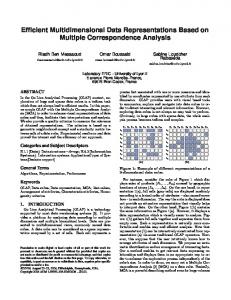
It follows that the segment of the boundary between P and Q under corresponding transform is a 0 1 -curve. Figure 2.3 demonstrates all descriptor points and their types of a digital set.

17


T

4

T3

T5

S1

S0

S

7

S

2

S6 S3

S 4 S

S

5

0

S1

S7

T2

T6

T

T0

T1

T7 T0

T1

7

Figure 2.3: Digital set “Letter A”. Descriptor points and their types are indicated.

18


Chapter 3 Digital Convexity The term of convexity is a central subject of many geometrical investigations. Particularly, in the application oriented disciplines of geometry it plays an important role. The basic constructions of digital geometry are discrete lines, discrete line segments and digitally convex sets. They belong since beginning of the research in digital geometry to the frequently examined objects.

3.1 Discrete Lines We adapt the definition of discrete lines introduced by J.-P. Reveillès [40].

Definition 3.1 A discrete line with a slope a b b 0 and pgcd a b 1, lower bound µ, arithmetical thickness ω is the set of grid points which satisfies the double diophantine inequality µ ax by µ ω

with all integer parameters. A (finite or infinite) subsequence of a discrete line is called a discrete line segment.

We denote the preceding discrete line D a b µ ω . We are mostly interested in na¨ıve lines which verify ω sup a b , we shall denote them D a b µ . Without loss of generality we may consider discrete lines under restrictions a b 0 and b. a b, therefore ω max a b The real straight lines ax by µ and ax by µ b 1 are called upper leaning line and lower leaning line of D a b µ , respectively. There are no grid points of the complement D a b µ between the upper and lower leaning lines and D a b µ . The grid points satisfying the leaning line equalities are called upper and lower leaning points. We remark that the distinction between lower and upper leaning points depends on the equation, there is here no geometrical invariancy. It can be shown [40] that a discrete line D a b µ with slope a b 1 has exactly one grid point on each vertical line. If a b 1 then the intersection between

19

20

Digital Convexity

D a b µ and any horizontal line is composed by b a or b a

1 successive grid points, where means the integer part. Thus, according to Proposition 3.2 (see below) and considering discrete line segments with minimal parameters a and b, we may denote UF (LF ) the upper (lower) leaning point of a discrete line segment with slope a b 1 whose x-coordinate is minimal. In the same way, we denote UL (LL ) the upper (lower) leaning point whose x-coordinate is maximal. An example in Figure 3.1 shows a segment of the discrete line D 5 8 4 with its leaning points and leaning lines.

UL

L

L

UF LF

Figure 3.1: Segment of discrete line D 5 8 4 . Dashed lines represent upper and lower leaning lines of the segment. Upper and lower leaning poins are indicated by pale and dark triangles.

A discrete line D a b µ , where 0 a b, satisfies the chord property and is 8-connected [8, 40]. It follows that a discrete line segment is a digital straight line segment in sense of Hübler, Klette, Voss [21]. The finite digital curves with the chord property are discrete line segments. There are infinite digital curves which satisfy the chord property and, however, are not discrete lines [20]. We collect some simple properties of discrete lines. The proof of the following proposition can be found in [40].

Proposition 3.1 A discrete line D a b µ with 0 a b is an 8-curve.

b is a 0 1 -curve.

This result implies that the movement from left to right along a discrete line with 0 a b occurs by using of two translations either x y x 1 y or x y x 1 y 1 . We have shown:

Proposition 3.2 Each discrete line D a b µ with 0 a

Since a discrete line D a b µ is an 8-curve the concept of levels and their lengths of D a b µ are justified, it coincides with the definition for a digital curve.

Digitally Convex Sets

21

Proposition 3.3 The lengths of horizontal levels of a discrete line D a b µ with 0 a b are different mostly by one.

Proof The intersection between D a b µ and any horizontal line is composed by b a or b a 1 which are possible lengths of the levels.

Proposition 3.4 Let D a b µ with 0 a b be a discrete line. Then the upper and lower leaning points of D a b µ belong to such horizontal levels of the discrete line which possess the maximal lengths. Proof Trivial. Clearly this proposition is not true for discrete line segments.

Proposition 3.5 Given a discrete line D a b µ with 0 a b. Assume lengths of the horizontal levels of D a b µ are i and i 1. Then i 1 1 ab 1i .

Proof The slope ab of the discrete line is at least i 11 whenever all horizontal levels have lengths i 1. Othewise, it can be at most 1i if all levels have lengths i.

3.2 Digitally Convex Sets In Euclidean geometry a set in d is said to be convex if whenever it contains two points, it also contains the line segment joining them. Already in two-dimensional case there were observed difficulties by direct transfer of this definition into digital circumstances (see e.g. [20]). In the literature there exist different types of digital convexity. The most common of them are studied in [22, 23, 24, 37]. We will introduce some useful concepts from ordinary geometry.

Definition 3.2 A polygonal curve Π V E in 2 consists of a cyclically ordered 2 and a set of edges E set of vertices V v 0 v1 vn V V . E is the set of all line segments joining vi and vi 1 , i 0 1 n 1. Usually it is assumed that there are finitely many vertices. Sometimes also infinite edges are allowed. A polygonal curve Π V E is said to be

bounded if V is a finite set and if there are no infinite edges; closed if each vertex belongs to exactly two edges; simple if two edges are either disjoint or meet in a vertex, and if vi

v j for i

Π

A polygonal set Π is a finite set of simple closed curves Π1 Π2 are mutually disjoint.

n

j.

which

22

Digital Convexity

2 and three successive vertices x y , Definition 3.3 Given a polygonal curve Π 1 1 x2 y2 and x3 y3 on Π. The point x2 y2 is a convex vertex of Π if the determinant

x2 y2

x1 x3 y1 y3

x2 y2

Definition 3.4 Let Π be a polygonal curve. A part of the curve is said to be a maximal convex part if it is consists of a set P P P of successive vertices of Π together with the lines joining them such that P and P are concave vertices of Π and P P P are convex vertices of Π. If Π has only convex vertices, the is positive. x2 y2 is a concave vertex of Π if the determinant is negative. If the determinant vanishes then points x1 y1 x2 y2 and x3 y3 are collinear.

1

2

1

2

3

k

k

k 1

only convex part of Π is Π itself. In this case Π is called convex curve. A maximal concave part of Π is defined in the same manner by replacing in the above definition the terms “convex” and “concave”.

We here have a perfect duality: If we replace a polygonal set by its complement, the orientation of the curve is reversed and maximal convex parts become maximal concave parts and vice versa. Furthermore, the common part of two successive maximal parts is one single edge of the curve. Let K κ1 κn be a segment of a discrete line D a b µ . The problem to determine the convex hull of the elements of K is solved in [9]. The convex hull of K is a closed polygonal curve which can be subdivided into two polygonal curves joining κ1 and κn : the lower frontier and upper frontier of the convex hull. It is clear that the lower leaning points of this segment belong to the lower frontier, upper leaning points belong to the upper frontier. How to detect all points of the lower and upper frontier is shown in [9, Proposition 3, p.120] (see also Proposition 4.3, p. 41). Since K is a segment of a discrete line the intersection of K and its convex hull consists only of elements of K . Moreover, all vertices of the lower and upper frontier of K are convex. These facts justify the following concept of digitally convex sets of d : d. Let denote convS the convex hull of S

Definition 3.5 A set S

d

is called digitally convex whenever S

d

convS

2 is digitally convex if and only if there exists a Corollary 3.1 A digital set S 2 such that Π 2 convex polygonal set Π S .

23

Fundamental Segments of 8-curves

Proof Trivial. Segments of discrete lines are simpliest examples for digitally convex sets. In general digitally convex sets are not necessarily 8-connected, e.g. the set consisting of x y and x 2 y 1 is digitally convex, but not 8-connected. Testing convexity of 8-connected digital sets in 2 can be restricted to testing convexity of their boundaries which can be subdivided into k k 1 mod 8 -curves (see Lemma 2.2, p. 15). In order to introduce convexity of digital curves we define:

Definition 3.6 Let K κ1 κn be a finite 0 1 -curve. K is said to be lower digitally convex (upper digitally convex) if there is no grid point between K and the lower (upper) frontier of the convex hull of K . The algorithm SegConv for testing convexity of digital curves from [9] can be applied for testing convexity of 8-connected sets (see Theorem 3.2, p. 29 and Theorem 3.3, p. 30). This algorithm has the linear time complexity.

3.3 Fundamental Segments of 8-curves

We consider a segment Σ of a discrete line D a b µ , where 0 a b, and x 1 y1 and xn yn are the first and last points of the discrete segment, respectively. Let us suppose that the point x y with x y xn 1 yn or x y xn 1 yn 1 is ¯ added to Σ. Is Σ Σ x y a discrete line segment and, if it is the case, that are its characteristics a¯ b¯ µ¯ ? Based on Theorem 3.1 (see below) linear Algorithm AddPoint describing solution of this problem was proposed in [8] (see also [9]). For this reason an indicator for each grid point x y called remainder was introduced. The remainder r x y shows the relationship between a point x y and a discrete line D a b µ .

Definition 3.7 The number

r x y ax

For a discrete line D a b 0 the remainder r x y represents within multiplicator a b Euclidean distance between x y and the real line ax by 0. Theorem 3.1 Let r x y be remainder at x y with respect to D a b µ . 1. If µ r x y µ b then x y D a b µ and Σ x y is a segment of the discrete line D a b µ . 2. If r x y µ 1 then Σ x y is a segment of the discrete line with slope U x y . by

is called remainder at x y with respect to D a b µ . 2

2

F

1 2

24

Digital Convexity

µ b then Σ x y is a segment of the discrete line with slope µ b then Σ x y is not a segment of a discrete 4. If r x y µ 1 or r x y 3. If r x y LF x y .

line.

Algorithm IV AddPoint adding a point P xP yP to the segment Σ of a discrete line D a b µ .

remainder axP byP ; if µ remainder µ b then if remainder µ then UL xP yP ; if remainder µ b 1 then LL xP yP ; else if remainder µ 1 then LF LL ; UL xP yP ; a yP yUF ; b xP xUF ; µ axP byP ; else if remainder µ b then UF UL ; LL xP yP ; a y P y LF ; b x P x LF ; µ axP byP b 1; else the point may not be added to the segment end end end

Now we are able to introduce fundamental segments of a 0 1 -curve.

Definition 3.8 Let K κ1 κn be a 0 1 -curve. Parameters a and b in discrete line segments considered below are assumed to be minimal. A part κ i κj is called a fundamental segment of K whenever one of the following conditions is true:

1. i 1, j n and κ1 κn is a segment of D a b µ . Then K consists of one single fundamental segment.

25

Convex and Concave Curves

3. i 1, j n and κ κ is a segment of D a b µ such that κ κ is not a segment of any discrete line. Here, κ κ is the last fundamental segment of K . 4. i 1, j n and κ κ is a segment of D a b µ such that κ κ and κ κ are not segments of any discrete line. The fundamental segment κ κ will be denoted F a b µ .

2. i 1, j n and κ1 κ j is a segment of D a b µ such that κ1 κj 1 is not a segment of any discrete line. Here, κ1 κ j is the first fundamental segment of K . i

n

i

i

i

i 1

n

i 1

j

n

j

j 1

i

j

By this definition the convex hull of a fundamental segment of K and the left or right added point consists at least of one grid point of the complement of K [9, Remark 6]. Hence, fundamental segments are maximal possible subsets of K belonging to discrete lines. Moreover, fundamental segments do not depend of the orientation of K . Assume a curve K possesses m fundamental segments. Then all fundamental segments can be ordered in the sense of the oriented curve, we mark these Fi a i b i µ i , i 1 m. It is clear that two successive fundamental segments have allways different slopes and their common part is not empty and it is always a segment of a discrete line. In addition, more than two fundamental segments can possess common parts of K . Clearly, decomposition of a 0 1 -curve into fundamental segments is unique. The problem to find this decomposition is equivalent with the problem to determine subsets of the curve having constant tangents. It can be computed within linear time [17]. In Figure 3.2 fundamental segments of a digital 0 1 -curve are indicated.

3.4 Convex and Concave Curves In Euclidean geometry the boundary of a polygonal set Π can be easily partitioned into maximal convex and concave parts by means of convex and concave vertices of Π. The partition of the boundary of a digital set into the meaningful parts is not a simple task. By Tietze’s theorem [45] convexity of a set in 2 can be decided locally in a time which is proportional to the length of the boundary of the set. In 2 one can easily deduce that convexity of a set cannot be decided locally [11]. So, it becomes an interesting question, how far one can decide whether a part of the boundary of a digital set is convex or concave by a method which is “as local as possible”. In [14] the idea was suggested to determine a corresponding polygonal representation of a digital set S using the concept of exposed points of S (see Definition 4.2, p. 37), the exposed points were defined also for non convex sets. The meaningful parts of the set were defined as meaningful parts of the corresponding

26

Digital Convexity F (1,3,−13) 6

F5(3,5,17) F (8,11,71) 4

F1(1,7,−5)

F (2,5,7) 2

F3(1,4,−1)

Figure 3.2: Fundamental segments Fi ai bi µi , i 1 6 of a digital curve. The first point of the curve is 0 0 . Lower bounds µi , i 1 6 of fundamental segments are computed with respect to 0 0 .

polygonal representation. The obvious and interesting fact is that the parts of the boundary of S between two successive exposed points are discrete line segments. In our considerations we use geometry of digital sets, especially, geometry of discrete line segments. We will introduce another approach how to define convex and concave parts of a digital curve using the concept of fundamental segments. Next definition shows that fundamental segments allow an adaption of the term convex and concave curve from continuous theory.

Definition 3.9 Let K be a 0 1 -curve and Fi ai bi µi , i 1 m are fundamental segments of K . The curve K is called convex (concave) whenever the sequence a a of the slopes of fundamental segments is increasing (decreasing), i.e. b jj b jj 11 aj bj

, 1 j m 1. In the case K is a discrete line segment it is both convex and concave.

aj bj

1 1

Since the sequence of fundamental segments does not depend of the orientation of K the concave curve is a convex one if the orientation of K is reversed. In the following considerations only convex case will be proved, the concave case can be formulated analogously and shown by duality. Lower leaning points of fundamental segments of convex curves are located not arbitrarily. Namely, they appear in the successive order on the curve. This statement is proved in the next proposition. We mark the x- and y-coordinate of a point P as xP and yP , respectively.

Proposition 3.6 Let K be a convex (concave) 0 1 -curve and Fi ai bi µi , i 1 m are fundamental segments of K . Then for lower (upper) leaning points holds x LL j x LF j 1 xUL j xUF j 1

27


for all 1

j m

1.

Proof Given fundamental segments F j a j b j µ j and F j 1 a j 1 b j 1 µ j 1 of K . Let Π be the polygonal set consisting of edges e1 : a j x b j y µ j b j 1 and e2 : a j 1 x b j 1 y µ j 1 b j 1 1 which are lower leaning lines of F j a j b j µ j and F j 1 a j 1 b j 1 µ j 1 . One single vertex V xV yV of Π is the intersection point of e1 and e2 . Obviously, K is above Π. Since the sequence of the slopes is increasing it holds xLL j xV and xV xLF j 1 .

In Figure 3.3 a convex curve with different locations of lower leaning points of fundamental segments is represented. F3(5,6,24) LL3

F (4,7,4) 2

L =L L2 F3

F1(2,5,−1) L LF1=LL1 F2

Figure 3.3: Convex curve and its lower leaning points of fundamental segments Fi ai bi µi , i 1 2 3. For lower leaning points holds xLL1 xLF2 and xLL2 xLF3 . The statement corresponding to Proposition 3.6 about succession of upper leaning points on convex curve is, generally, not true. An example is shown in Figure 3.4. U

L3

U

L2

U UF1=UL1 UF2

F3

F (3,5,16) F (3,8,0) 2

3

F1(3,10,−9)

Figure 3.4: Convex curve and its upper leaning points of fundamental segments Fi ai bi µi , i 1 2 3. For upper leaning points UL1 and UF2 holds xUL1 xUF2 , however, for UL2 and UF3 holds xUL2 xUF3 .

If for leaning points LL j and LFj 1 of F j a j b j µ j and F j 1 a j 1 b j 1 µ j 1 of a convex curve K holds xLL j xLF j 1 then, obviously, LL j LFj 1 is a vertex of

28

Digital Convexity

the lower frontier of the convex hull of K . Before the situation xLL j xLF j 1 will be examined we introduce a concept of supporting lines. A real line L is called a lower supporting line in P K (briefly, LSL) if P L and there exists a (continuous) neighborhood N P of P such that all elements in K N P are lying on or above L. A convex curve K with a fundamental segment F a b µ , whose leaning points are LF and LL , is lying on or above lower leaning line of F a b µ . Hence, ax by µ b 1 is a LSL in LF , LL and all grid points which belong to K on the real line segment LL LF . Moreover, there exists no grid point between the segment LF LL of K and LF LL . If the whole curve K is on or above a LSL, then the LSL is also called a global lower supporting line (briefly, GLSL). If an arbitrary 0 1 -curve K with m fundamental segments Fi ai bi µi and a GLSL in P K such that P LF1 LLm are given, then P belongs to one of lower leaning lines of Fi ai bi µi . Obviously, there can exist a GLSL in P which is before LF1 or after LLm , however, this case does not play any role for our further considerations.

m be Proposition 3.7 Let K be a convex 0 1 -curve and Fi ai bi µi , i 1 fundamental segments of K . Let us assume xLL j xLF j 1 for some 1 j m 1. Then there is no grid point between fundamental segments F j a j b j µ j and F j 1 a j 1 b j 1 µ j 1 and the polygonal set with successive edges e1 : a j x b j y µ j b j 1, e2 : the real line through LL j and LFj 1 , and e3 : a j 1 x b j 1 y µ j 1 b j 1 1.

Proof Real lines e1 and e3 describe lower leaning lines of fundamental segments F j a j b j µ j and F j 1 a j 1 b j 1 µ j 1 . It follows that there is no grid point between the polygonal set with both edges, whose intersection point is the vertex V , and these fundamental segments. Thus, we only must show that elements of LL j LFj 1 are lying above e2 . Let us assume P K is one single point inside the triangle with vertices LL j , LFj 1 , V . Illustration is given in Figure 3.5.

LLj+1

LFj+1 LFj

L

Lj

P V

Figure 3.5: Illustration to Proposition 3.7.

29


We deduce that there exists a GLSL in P. Hence, P is on one of lower leaning lines of fundamental segments, but not on e1 or e3 , i.e. there must exists a fundamental segment between F j a j b j µ j and F j 1 a j 1 b j 1 µ j 1 . It leads to a contradiction that both fundamental segments are successive. Analogously, the case, where more than one points are inside the triangle, leads to this contradiction.

Now we are able to show the equivalence between convex and lower digitally convex curves.

Proof Let F a b µ , i 1 m be fundamental segments of K . 1. Let us assume K is convex. We consider a polygonal curve Π consisting of vertices of the lower frontier of the convex hull of F a b µ before L , intersection points of lower leaning lines of F a b µ and F a b µ , j 1 m 1 and vertices of the lower frontier of the convex hull of F a b µ after L . Since K is convex, Π possesses increasing slopes and there is no grid point between Π and the curve K . By Proposition 3.6, for two successive fundamental segments F a b µ and F a b µ holds x x . If x x L is a vertex of Π. In the case x x , then L for the slope s of the real line segment L L holds s . According to Proposi tion 3.7, there is no grid point between L L and L L . In this case, we modify the polygonal curve Π by replacing the vertex which is intersection point of lower leaning lines of F a b µ and F a b µ by vertices L and κ1 κn be a 0 1 -curve. The curve K is convex if and Theorem 3.2 Let K only if K is lower digitally convex. i

i

i

i

1

j

j

j

1

1

j

1

j 1

F1

j 1

j 1 m

j 1

m

m

m

Lm

j

LL j

LF j

Lj

1

j

j

Fj

j

j 1

j 1

j 1

Fj

1

Lj

j

j

j

aj bj

aj bj

Fj

j

LF j

j 1

LF j

1

1

1 1

Lj

1

j 1

LL j

LL j

1

Lj

j

j 1

Fj

1

Lj

j 1

LFj 1 . Hence, modified Π has all successive vertices of the lower frontier of the convex hull of K and there is no grid point between K and the frontier. 2. We assume that there is no grid point between K and the lower frontier of the convex hull of K . In the case m 1, the statement is, obviously, true. If m 1, then the curve K possesses at least two fundamental segments. It is clear that the points LF1 and LLm are always vertices of the lower frontier. Let us assume m 2 and slopes of F1 a1 b1 µ1 and F2 a2 b2 µ2 are decreasing, i.e. LF1 and LL2 are vertices of the lower frontier and there exists no other vertex between them. Then, there must be at least one grid point between L F1 LL2 and LF1 LL2 . Otherwise, LF1 LL2 is a discrete line segment belonging to the curve contradicting the consecutivity of F1 a1 b1 µ1 and F2 a2 b2 µ2 . For m 2 the similar arguments lead to a contradiction when we assume that slopes of F j a j b j µ j and F j 1 a j 1 b j 1 µ j 1 , 1 j m 1 are decreasing.

Remark 3.1 From the first part of the proof to Theorem 3.2 we deduce that lower leaning points LF1 LL1 LF2 LL2 LFm LLm of a convex curve K with fundamen-

30

Digital Convexity

tal segments Fi ai bi µi , i 1 m are vertices of the lower frontier of the convex hull of K between LF1 and LLm . By duality UF1 UL1 UF2 UL2 UFm ULm are vertices of the upper frontier between UF1 and ULm of a concave curve.

Let us concentrate on linear transforms T k for k end of Section 2.

0 7

described at the

2. Assume S possesses only Theorem 3.3 Given an 8-connected digital set S T -descriptor points. Then the set S is digitally convex if and only if the following conditions are true:

2. The parts of the boundary of S between descriptor points of type k and k 1 mod 8 , k 1 3 5 7 under the transform T are concave curves. Proof We consider an 8-connected digital set S . Using Scherl’s descriptors it is possible to partition the boundary of S into k k 1 mod 8 -curves. For k 0 2 4 6 the part of the boundary under T is a 0 1 -curve, the interior of the set S is on the left side, for k 1 3 5 7 it is on the right side. In the first situation we must consider the lower frontier of the curve, in the second the upper frontier. 1. Let S be digitally convex. Then vertices of the lower (upper) frontier of the described above 0 1 -curve for k 0 2 4 6 (k 1 3 5 7) are vertices of convS and there exists no grid point between the frontier and the curve. By Theorem 3.2 the curve is convex (concave). 2. Assume the 0 1 -curves for k 0 2 4 6 (k 1 3 5 7) of S are convex

1. The parts of the boundary of S between descriptor points of type k and k 1 mod 8 , k 0 2 4 6 under the transform T k are convex curves. k

2

k

(concave). We consider a polygonal set Π having vertices of the lower (upper) frontier of the convex (concave) curves. There is no grid point between curves and 2 the lower (upper) frontier of the convex hull of curves. Thus, we deduce Π S . Since S possesses only T -descriptor points the polygonal set Π is convex. It follows that S is digitally convex.

3.5 Decomposition of Curves into Meaningful Parts

Let us consider a digital 0 1 -curve K . By means of fundamental segments of K and their slopes we are able to define convex and concave parts of K which are maximal.

Definition 3.10 Let K be a finite 0 1 -curve and Fi ai bi µi , i 1 m are fundamental segments of K . A part consisting of successive fundamental segments Fu au bu µu , ,Fv av bv µv , 1 u v m is called a maximal convex part of K whenever one of the following conditions is true:

31

Decomposition of Curves into Meaningful Parts

1. u 2. u

1, v

4. u 1, v 3. u

1, v

1, v

aj bj

m and m,

au bu

m,

av bv

m,

au bu

1 1

,1

au av bu , bv

1 1

av bv

1 1

aj bj

j m

av bv

1 1

and

aj bj

au bu

and

aj bj

1 1

and aj bj

1

aj bj

1

1

1

1. aj bj

aj bj

1 1

for all u

for all 1

j v

for all u

j m

j v

1.

1. 1.

A maximal concave part of K is defined in the same manner by replacing the signs “ ” and “ ” in the above definition.

It is clear that a convex (concave) curve consists exactly of one single maximal convex (concave) part. The maximal parts of a curve K overlap each other. If K is neither convex nor concave then each its maximal convex and concave part has at least two fundamental segments. The common component of two successive meaningful parts consists of exactly one fundamental segment. Let us concentrate on Figure 3.6, where the curve from Figure 3.2 is represented again. The slopes of 6 successive fundamental segments are abii 0 1429, 0 4, 0 25, 0 7273, 0 6, 0 3333. We deduce that the curve possesses four maximal parts: convex consisting of F1 a1 b1 µ1 and F2 a2 b2 µ2 ; concave with F2 a2 b2 µ2 and F3 a3 b3 µ3 ; convex with F3 a3 b3 µ2 and F4 a4 b4 µ4 ; concave consisting of F4 a4 b4 µ4 , F5 a5 b5 µ5 and F6 a6 b6 µ6 . It is an interesting observation that there exists a common point P of more than two maximal convex and concave parts.

(F ,F ,F ) 4 5 6

(F ,F ) 2

P

3

( F3 , F4 ) ( F1 , F2 )

Figure 3.6: Maximal convex and concave parts of the curve from Figure 3.2. The point P belonging to each maximal part is indicated.

Given a digital set S in 2. We are interested in partitionning the boundary of S into maximal possible meaningful parts. We are able to decompose the boundary into k k 1 mod 8 -curves using Scherl’s descriptors. First we can find the predecomposition in the following manner:

32

Digital Convexity

Figure 3.7: Maximal convex and concave parts of “Letter A” indicated by dark and pale triangles, respectively.

33

Fundamental Polygonal Representations of Digital Curves

1. The segments of the boundary of S between descriptor points of type k and k 1 mod 8 , k 0 2 4 6 are convex (concave) parts of S whenever they are convex (concave) parts of the corresponding 0 1 -curve.

2. The segments of the boundary of S between descriptor points of type k and k 1 mod 8 , k 1 3 5 7 are convex (concave) parts of S whenever they are concave (convex) parts of the corresponding 0 1 -curve.

Obviously, the pre-decomposition possesses no maximal possible parts. Using the fact that T -descriptor points always belong to a convex part and S-descriptor points to a concave part we can determine the maximal convex and concave parts of the boundary of S . In the case we can replace T - and S-descriptor points by reversing the orientation we have again the perfect duality: the convex parts will become the concave and vice versa. In Figure 3.7 the partition of the boundary of a digital set into convex and concave parts is shown.

3.6 Fundamental Polygonal Representations of Digital Curves

In this section we shortly discuss an important application of decomposition curves into fundamental segments. Let K be a finite 0 1 -curve and F a b µ a fundamental segment of K . The (whole) segment F a b µ is located above the lower leaning line ax by µ b 1 and under the upper leaning line ax by µ. Moreover, there is no grid point between the segment and the leaning lines. We consider two successive fundamental segments F j a j b j µ j and F j 1 a j 1 b j 1 µ j 1 . The common part of the segments is not empty and located above the both lower leaning lines a j x b j y µ j b j 1 and a j 1 x b j 1 y µ j 1 b j 1 1, also under the both upper leaning lines a j x b j y µ j and a j 1 x b j 1 y µ j 1 . Hence, the segments F j a j b j µ j and F j 1 a j 1 b j 1 µ j 1 is above (under) the polygonal curve Π with edges given by mentioned real lines and the vertex given by their intersection point, respectively. There exists no grid point between the polygonal curves and the fundamental segments. These considerations allow to introduce a concept of fundamental polygonal representations:

Definition 3.11 Let K be a finite 0 1 -curve and Fi ai bi µi , i 1 m are fundamental segments of K . A polygonal curve Π with edges given by lower (upper) leaning lines of Fi ai bi µi and vertices given by their intersection points in successive order is called lower (upper) fundamental polygonal representation of K.

Figure 3.8 demonstrates the upper and lower fundamental polygonal representations of the curve from Figure 3.2. We collect some simple properties of fundamental polygonal representations:

34

Digital Convexity

Figure 3.8: Fundamental polygonal representations of the curve from Figure 3.2. 1. There is no grid point between fundamental polygonal representations and the digital curve. 2. Vertices of fundamental polygonal representations are, generally, not grid points. 3. The lower (upper) fundamental polygonal representation of a convex (concave) digital curve possesses only convex (concave) vertices. 4. The fundamental polygonal representations have the same convexity properties as the digital curve. 5. The representations are translations of each other and have the same Euclidean lengths.

6. If for lower (upper) leaning points of fundamental segments F i ai bi µi , i 1 m of a convex (concave) curve holds LL j

LF j

1

U Lj

UFj

1

1

j m

1

then vertices of the lower (upper) fundamental polygonal representation are vertices of the lower (upper) frontier of the convex hull of K between L F1 and LLm (UF1 and UFm ).

Chapter 4 Polygonal Representations of Digital Sets In Section 3.2 we introduced such concepts of Euclidean Geometry and Convexity Theory like polygonal curves, polygonal sets, convex and concave vertices of polygonal curves. In the plane 2 the boundary of a polygonal set can be decomposed into convex and concave parts in an obvious way. On the other hand, we have shown how to partition the boundary of a digital set in 2 into meaningful parts by means of Scherl’s descriptors and fundamental segments. However, in spite of the precision, proposed decomposition has also different disadvantages, e.g. before the set can be partitioned into convex and concave parts one needs information about slopes of fundamental segments, more than two parts can possess common elements, the decomposition is less suitable for our visual system. Therefore, the aim of this chapter is to describe digital sets by means of polygonal sets in 2 with corresponding convexity properties. We state some important characteristics of polygonal sets in the plane 2 .

1. For a polygonal set we can define in an obvious way such topological concepts like connected components, simply connected polygonal sets or holes of the set. 2. The famous Jordan Curve Theorem states that any (bounded) simple closed polygonal curve Π separates the plane into the interior and the exterior with respect to the curve. More formally: The set 2 Π consists of exactly two disjoint connected components. One of them is declared as the interior and the other as the exterior with respect to Π. 3. In the definition of convex and concave parts of a polygonal curve we have a perfect duality: If we replace a polygonal set by its complement, the orientation of the boundary is reversed and convex parts become concave parts and vice versa. 35

36

Polygonal Representations of Digital Sets

2. A polygonal representation of S is a Definition 4.1 Given a digital set S polygonal set Π V E with vertices V and edges E such that

x

S

x

Π

2

A polygonal set representing a digital set is not unique. We are free to require a number of additional characteristics. The polygonal representation Π of a digital set S is said to be

discrete if all vertices of Π are in

2;

faithful if convex parts of the boundary of S correspond to convex parts of the boundary of Π, and if the same is true for concave parts.

2 may belong to more than Remark 4.1 A boundary point of a digital set S two maximal parts. To be more precise, a representation Π is faithful if the succession of convex and concave parts of the boundary of S corresponds to the succession of convex and concave parts of the boundary of Π.

The chain code representation of the boundary of a digital set is a discrete polygonal representation having a maximal number of vertices. It is, however, not faithful. Using fundamental polygonal representations of the boundary of a digital set S (see Section 3.6) we are able to determine a faithful polygonal representation of S . Generally, this representation is not discrete. In our further considerations we are mostly interested in polygonal representations of digital sets which are both discrete and faithful. We distinguish between two situations: first, the polygonal representations of digitally convex, and, second, of non convex sets. The first case is far better studied in [9, 14, 21]. Evidently, the unique discrete and faithful polygonal representation of a digitally convex set is the convex hull of the set. Linear algorithms for determination the convex hull of a digital set and testing convexity are developed [9, 21]. We introduce another implementation which is based on the concept of fundamental segments of a digital curve. Since in the literature it is more usual to consider lower polygonal representations, in Section 4.1 convex curves and their lower polygonal representations are studied. In Section 4.2 upper representations of general curves are considered (in this case upper representations are convenient for computation). Furthermore, we will show the existence of a linear algorithm which detects discrete polygonal representation of a digital set with “only few” uncorresponding parts.

4.1 Convex Case

η with η is ηequipped and

We need concepts from ordinary convexity theory. Assume Euclidean geometry, i.e. to an arbitrary pair of vectors x

d

1

2

d

37

Convex Case

ζ ζ ζ the inner product x y

y

1

2

d

d

∑ η jζ j

j 1

is assignet.

d . A point x Definition 4.2 Given a convex set S S is an exposed point of S 0 if there exists a nonzero vector x such that x0 x x x for all x S x0 . d is digitally convex then x is an exposed point of S if it is an exposed If S 0 point of convS .

It is well known from convexity theory that the convex hull of a polygonal set is the convex hull of its exposed points [46]. On the other hand vertices of a convex polygonal set are exactly its exposed points. For digitally convex sets there exists a simple characterization of exposed points (the following lemma is proved in [15]):

2 be a digitally convex set. A point P Lemma 4.1 Let S S is an exposed point of S if and only if P is a vertex of each discrete polygonal representation Π of S .

Lemma 4.1 can be shown also for the digitally convex sets from d . The discrete polygonal representation must be understood as a polyhedral representation with all vertices in d . d and x is a vertex of each Proof 1. Assume given a digitally convex set S 0 discrete polyhedral representation of S . Since convS is a discrete polyhedral representation of S so x0 is also a vertex of convS . The exposed points of a convex set are exactly its vertices. Hence, x0 is an exposed point of convS and of S as well. 2. Let Π be a discrete polyhedral representation of S . If x0 is an exposed point of S then there exists a nonzero vector x such that x0 x x x for all d x S x0 , also for all x Π x0 . For

H:

x d x0 x

xx

holds Π H. The point x0 is a (topological) boundary point of H and, consequently, it is also a boundary point of Π. In d this implies that x0 belongs to a facet of Π which is d 1 face of Π (definitions see Section 5.5). The point x0 is exposed, it must belong to the boundary of the facet, thus, to the d 2 face. In all cases x 0 belongs to the boundary of i-face, i 1 d 1. We deduce that x0 is a vertex of Π.

These considerations justify the following definition for exposed points of digital sets which are not necessarily digitally convex.

38


2. A point P Definition 4.3 Given a digital set S S is called an exposed point of S whenever a discrete and faithful polygonal representation Π of S exists and P is a vertex of Π.

It is clear that exposed points in Definitions 4.2 and Definition 4.3 in the case when S is digitally convex are the same points. Thus, exposed points of a digitally convex set S are exactly vertices of the convex hull of S . Our goal is to detect all successivelly ordered exposed points on the boundary of an 8-connected digitally convex set. Assume, S is 8-connected and digitally convex, the boundary of S is oriented. Then there exists the unique polygonal representation which is discrete and faithful. This representation is the convex hull convS of S . Since the boundary of a digitally convex set possesses only T -descriptor points and can be decomposed into convex and concave 0 1 -curves (see Theorem 3.3, p. 30), we may restrict our considerations to convex 0 1 -curves. The polygonal representation of a 0 1 -curve K κ1 κn can be subdivided into two polygonal curves between κ1 and κn : lower and upper polygonal representation. Thus, computation exposed points of a digitally convex set can be restricted to computation vertices of discrete and faithful lower polygonal representations of convex curves. Obviously, the discrete and faithful lower polygonal representation of a curve K is lower frontier of the convex hull of K . Assume Fi ai bi µi are fundamental segments of K with lower leaning points LFi and LLi , i 1 m. Then by Remark 3.1, p. 30 vertices of the discrete and faithful polygonal representation between LF1 and LLm coincide with leaning points LF1 LL1 LF2 LL2 LFm LLm of fundamental segments of K . However, for computation vertices of the lower polygonal representation it is not recommendable to determine all fundamental segments of K and their leaning points. In spite of linearity, this technique is applicable only to convex curves. For an arbitrary curve such algorithm is not suitable. We will show how to find leaning points of fundamental segments (within linear time) without computation fundamental segments. In convex as well as in general case we are mostly interested in leaning points of fundamental segments which are last (or, by duality, first) points of horizontal levels of K .

Proposition 4.1 Let K κ1 κn be a convex (concave) 0 1 -curve which is not a segment of a horizontal or diagonal grid line and Fi ai bi µi , i 1 m are fundamental segments of K . Then the lower (upper) leaning points L Fi and LLi (UFi and ULi ) for all 1 i m are last (first) points of horizontal levels of K . Proof Since the lower leaning line of a fundamental segment is a GLSL (global lower supporting line) of K , the proposition is trivially true.

The linear algorithm for detection vertices of the lower polygonal representation of a convex 0 1 -curve K with fundamental segments Fi ai bi µi , i 1 m

39

Convex Case

(not known) can be construct on the basis of Algorithm AddPoint. We apply Algorithm AddPoint to K and if the situation “the point may not be added to the segment” appears then the algorithm will be restarted at the last leaning point L L . This procedure is presented in Algorithm MainLoop. A similar algorithm was proposed in [9] for computing the convex hull of a digitally convex set.

Algorithm V MainLoop computing (some) vertices of the lower polygonal representation of a 0 1 -curve K κ1 κn .

V vertices of the lower polygonal representation START κ1 ; start point repeat Determine the segment START κ j of a discrete line D a b µ such that j n or START κ j 1 is not a segment of any discrete line; V V L F LL ; if START κ j 1 is not a segment of any discrete line then START LL ; else ST OP; end until ST OP;

The algorithm can be used for computation upper polygonal representations of concave curves when the lower leaning points are replaced by upper leaning points, i.e. following lines have to be changed: V

V

LF

LL ;

by V

LL ;

by

V

UF UL ;

and START

START

UL ;

The described technique is similar to method for segmentation digital curves into discrete line segments by Debled-Rennesson and Reveillès [8]. The latter algorithm is linear, the both algorithms differ only in the points, where they are restarted. We deduce that Algorithm MainLoop is linear, too. The next proposition shows the principle the algorithm MainLoop works if the given 0 1 -curve is convex.

Proposition 4.2 Let K κ κ be a convex 0 1 -curve and F a b µ , i 1 m are fundamental segments of K . Then L F a b µ for all 1 j m 1. If K is concave then U F a b µ for all 1 j m 1. Proof By Proposition 3.6 one has x x for all 1 j m 1. In the case x x the statement of the proposition is trivially true. We concentrate on the situation x x . Assume L F a b µ for some 1

n

i

Lj

Lj

j 1

j 1

LL j

LL j

LF j

j 1

LF j

j 1

j 1

j 1

j 1

j 1

j 1

j 1

1

1

LL j

LF j

1

Lj

j 1

i

i

j 1

i

40 1


K between lower leaning line of L (see sketch in Figure 4.1).

j m 1. Then there exists a grid point P F j 1 a j 1 b j 1 µ j 1 and the segment LL j

Lj

1

L

Lj+1

LFj+1 L

LFj

Q

Lj

P

Figure 4.1: Illustration to Proposition 4.2

Remark 4.2 By symmetry it holds L F a b µ for convex and U F a b µ for all 1 j m 1 for concave curves. Assume Algorithm MainLoop is applied to a convex 0 1 -curve K and the leaning points L and L are detected in some repeat-loop. According to Proposition 4.2 one has L F a b µ . Since x x the algorithm

By the symmetry there is a grid point Q K between lower leaning line of F j a j b j µ j and the segment LFj LFj 1 . We deduce that LFj LF j 1 and LL j LL j 1 are not segments of any discrete line. Then there exists a fundamental segment F a b µ of K such that F a b µ LFj 1 LL j 1 1 , i.e. F a b µ is a fundamental segment whose first point is lying after L Fj and last point is lying before LL j 1 . It leads to a contradiction that F j a j b j µ j and F j 1 a j 1 b j 1 µ j 1 are successive. Lj

j

j

j

j

1

j

j

j

Lj

1

j

Fj

Lj

Lj

j 1

j 1

j 1

LL j

j 1

LF j

1

detects by starting at LL j either the leaning points LFj 1 and LL j 1 , or LFj 2 and LL j 2 is also possible. An example (here, the dual case for concave curve and its upper polygonal representation), where the latter situation appears, is demonstrated in Figure 4.2. In such situations Algorithm MainLoop fails. The solution of this problem is described in [9]. Let r x y ax by be remainder at x y with respect to a discrete line D a b µ . We consider a 0 1 -curve K κ1 κn which is a segment of the discrete line D a b µ . One has, obviously, r LF r LL and r UF r UL . The lower and upper leaning lines are global lower and upper supporting lines of K . Hence, for all κi , i 1 n holds r LF r LL r κi r UF r UL .

Proposition 4.3 Given a 0 1 -curve K κ κ which is a segment of a dis1

n

crete line. Then the vertices of the lower (upper) frontier of K are following points:

1. κ1 , κn and lower (upper) leaning poins LF and LL (UF and UL ) of the curve K;

41

General Case UL3 U =U F2 L2

U

F3

UL1 UF1

F2(3,8,−11)

F (3,10,−20) 3

F1(3,5,0)

Figure 4.2: An example, where Algorithm MainLoop fails. The vertex UF2 UL2 of the discrete and faithful upper polygonal representation of a concave curve will be not detected.

3. between L and κ (U and κ ): the maximal sequence of the points P , i 1 k such that r κ r P r P r L (r κ r P r P r U ). 2. between κ1 and LF (κ1 and UF ): the maximal sequence of the points Pi , r Pk r LF (r κ1 r P1 i 1 k such that r κ1 r P1 r Pk r UF );

L

n

L

n

n

k

i

1

k

L

n

1

L

Situations described in this proposition are visible in Figure 4.3. Points indicated in bold style justify Proposition 4.3. We modify Algorithm MainLoop for concave curves and their discrete and faithful upper polygonal representations (in general case the upper polygonal representation is convenient for computation, see Section 4.2, Remark 4.3). In each repeatloop we test if elements between start-point and the detected first upper leaning point UF satisfying Proposition 4.3 exist. In this way we will also detect vertices of the polygonal representation before UF1 . Furthermore, we must test if some vertices of the polygonal representation after ULm exist. Algorithm UpPolRep (on p. 43) detects all vertices of the discrete and faithful upper polygonal representation of a concave 0 1 -curve. Obviously, the algorithm has the complexity O n . The described technique is similar to the method for testing convexity from [9]. There is another proposal how to detect all exposed points of a digitally convex set introduced in [14]. It leads also to a linear algorithm.

4.2 General Case By digitally convex sets the existence of exposed points is guaranted. Moreover, exposed points are uniquelly given. In the general case the digital sets must be tested if a faithful and discrete polygonal representation really exists. On the other hand, as

42

Polygonal Representations of Digital Sets UL −4 −1 −3 2 0 −2 3 −4 1

LL

−1 −3 2 0 UF

−2 3 −4 1

L

F

−1 −3 2 0

Figure 4.3: Convex hull of a segment of the discrete line from Figure 3.1. The remainder of each point is represented. The dark voxels show upper and lower leaning points. Convex hull of the segment is convex hull of points indicated in bold style with following remainders 0 2 3 3 2 1 4 4 3 0 (beginning by first point of the segment in the order given by left hand side orientation).

it will be demonstrated below, some sets which are not digitally convex can possess more than one of such representations. It means that in Definition 4.3 exposed points of a digital set depend on a discrete and faithful polygonal representation of the set. Exposed points of some representation are not necessarily exposed points of the other. Let us consider a convex (concave) 0 1 -curve K κ1 κn . There exists the discrete and faithful lower (upper) polygonal representation of K , it is lower (upper) frontier of the convex hull of K with only convex (concave) vertices. Exists an upper (lower) polygonal representation which is discrete and faithful of a convex (concave) curve, i.e. a discrete representation having only convex (concave) vertices? The existence of a faithful upper (lower) polygonal representation was shown in Section 3.6. It is upper (lower) fundamental polygonal representation of K . However, this representation is in general not discrete. The following proposition shows that the curves which do not possess disrete and faithful polygonal representations are not exceptional.

Proposition 4.4 Let K κ1 κn be a convex (concave) 0 1 -curve which is not a segment of a horizontal or diagonal grid line. If for the chain code direction holds

1 (ν κ κ 0), or 2. ν κ κ 0 (ν κ κ 1)

1. ν κ1 κ2 n 1

1

n

2

n 1

n

43

General Case

AlgorithmVI UpPolRep computing vertices of the upper polygonal κ1 κn . representation of a 0 1 -curve K

V vertices of the upper polygonal representation START κ1 ; start point repeat Determine the segment START κ j of a discrete line such that j or START κ j 1 is not a segment of any discrete line; V V maximal sequence Pi 1 k between START and UF satisfying Proposition 4.3; V V UF UL ; if START κ j 1 is not a segment of any discrete line then START UL ; else ST OP; end until ST OP; V maximal sequence Pi 1 k between UL and κn satisfying V Proposition 4.3;

n

then there exists no discrete and faithful upper (lower) polygonal representation of the curve K .

Proof Assume the curve is convex. If the chain code direction ν κ 1 κ2 1 then, obviously, there exists an element κi , i 2 which belongs to each upper discrete polygonal representation of K , since the slope through κ1 and κi is 1. It follows that the vertex κi is always concave. An example is demonstrated in Figure 4.4 (see p. 46). Here, the chain code is ν κ1 κ2 1 and i 2. The point κ2 is a concave vertex of each upper discrete polygonal representation. Other cases can be shown analogously.

To show more examples, where curves do not possess discrete and faithful polygonal representations, we consider the first F1 a1 b1 µ1 and last Fm am bm µm fundamental segments of a convex (concave) curve K . It is possible that the situations described in Proposition 4.3 appear. It follows that the sequences of points Pi between κ1 and UF1 or ULm and κn (between κ1 and LF1 or LLm and κn ), if not empty, belongs to each discrete upper (lower) polygonal representation of K and vertices Pi are concave (convex). Hence, also here there exists no discrete and faithful upper (lower) polygonal representation of the curve K . For example, the vertices described in Proposition 4.4 belong to the sequence Pi . The elements of Pi are vertices of each discrete polygonal representation and by Definition 4.3 are not exposed, however, they are exposed points in sense of [14]. These facts lead to the idea of defining exposed points locally, that means between first leaning point of first fundamental segment and last leaning point of last

44


fundamental segment:

Definition 4.4 Given a 0 1 -curve K κ1 κn . Let Fi ai bi µi , i 1 m be fundamental segments of K . A point P K is called a locally exposed point of K whenever one of the following conditions is true:

1. The point P is a vertex of each upper (lower) discrete polygonal representation. 2. There exists a discrete upper (lower) polygonal representation Π such that between UF1 and ULm (LF1 and LLm ) the convex and concave parts of Π correspond to the convex and concave parts of K , and P is a vertex of Π. 3. There exists no upper (lower) discrete and faithful polygonal representation between UF1 and ULm (LF1 and LLm ), and P is a vertex of a discrete upper (lower) polygonal representation Π of K such that the number of uncorresponding parts in Π is minimal. Unlike the convex case, where we considered only the leaning points of fundamental segments, in the general case there can exist exposed points which are not necesserily leaning points of fundamental segments. Moreover, we have again to treat different locations of upper and lower leaning points of fundamental segments Fi a i b i µ i , i 1 m of a curve K . It is possible that points UFi or LLi are lying inside horizontal levels of K . However, it is always true that the first upper leaning point UF1 of the first fundamental segment is the first point of a horizontal level, the last lower leaning point LLm of the last fundamental segment is the last point of a horizontal level.

Proposition 4.5 Let K κ1 κn be a 0 1 -curve which is not a segment of a horizontal or diagonal grid line and Fi ai bi µi , i 1 m are fundamental segments of K . Then upper (lower) leaning points ULi (LFi ) for all i 1 m are first (last) points of horizontal levels of K , i.e. points of levels with minimal (maximal) x-coordinate.

Proof In general, the first and last element of a fundamental segment can be located inside horizontal levels of K . Since the whole segment is lying under the upper leaning line, it is possible that UFi , i 2 m is the first element of the segment, hence, is lying inside a horizontal level. However, ULi , i 1 m must be the first point of a horizontal level. Analogously, the mentioned segment is above the lower leaning line. Then LLi , i 1 m 1 can be located inside a horizontal m is allways the last point of a horizontal level of K . level, however, LFi , i

Remark 4.3 A problem in the general case is the fact that leaning points of successive fundamental segments can be successive elements of K or not (see Figure 3.4, p. 27), and may be located inside horizontal levels.

45

General Case

The situation, where some leaning points of fundamental segments lying inside horizontal levels of K , becomes much simplificated if we use the fact that fundamental segments of a 0 1 -curve K κ1 κn do not depend of the orientation and by Proposition 4.5 leaning points ULi and LFi , i 1 m are first and last points of horizontal levels, respectively. A lower polygonal representation of K is one from all upper polygonal representations of the 0 1 -curve K¯ with reversed orientation defined as follows:

K¯ κ κ

n

1

1 0

0 1

Hence, our considerations can be restricted to upper polygonal representations of digital curves that is convenient for computation. We will show that the existence of a polygonal representation which is discrete and faithful depends on the locations of leaning points of successive fundamental segments.

Lemma 4.2 Given a convex 0 1 -curve K κ1 κn . Let Fi ai bi µi , i 1 m, m 2 be fundamental segments of K . If upper leaning points of fundamental segments F j a j b j µ j and F j 1 a j 1 b j 1 µ j 1 for some 1 j m 1 satisfy xUL j xUF j 1 then there exists no discrete and faithful upper polygonal representation of the curve K . Moreover, there exists at least one point P UL j UFj 1 which is a concave vertex of each discrete polygonal representation.

Proof We treat two possibilities yUL j yUF j 1 and yUL j yUF j 1 (yUL j yUF j 1 is not possible) and show that in the both cases the discrete and faithful polygonal representation does not exist. 1. The restriction yUL j yUF j 1 means that the leaning points UL j and UFj 1 belong to the same horizontal level of K . Obviously, the predecessor of UFj 1 is located above the upper leaning line a j 1 x b j 1 y µ j 1 of the fundamental segment F j 1 a j 1 b j 1 µ j 1 . It follows that the first element of this fundamental segment is also the first leaning point UFj 1 . We check the possible discrete polygonal representations. The slope of the real line through UL j and UFj 1 is 0. The representation with vertices UFj ,UL j ,UFj 1 ,UL j 1 is not faithful, such one with vertices UFj ,UL j ,UL j 1 is not allowed. Furthermore, it is clear that the element UL j , which is by Proposition 4.5 the first point of a horizontal level of K , is a concave vertex of each discrete upper polygonal representation. 2. Assume yUL j yUF j 1 . We distinguish between different locations of the intersection point x y of upper leaning lines a j x b j y µ j and a j 1 x b j 1 y µ j 1. If x xUL j (an example see Figure 4.4, the intersection point x y of upper leaning lines is indicated) then UFj 1 F j a j b j µ j . We deduce that UFj 1 cannot be the first point of the fundamental segment F j 1 a j 1 b j 1 µ j 1 . It follows that

46


UFj 1 is the first point of a horizontal level and UFj 1 or the point P between UL j and UFj 1 satisfying Proposition 4.3 is a concave vertex of each upper discrete polygonal representation. UFj+1=ULj+1 P (x,y) U

Lj

UFj

F

(5,8,0)

j+1

Fj(1,3,−2)

Figure 4.4: Dashed line represents the upper leaning line of F j 1 a j 1 b j 1 µ j 1 . Polygonal set with vertices UFj UL j UFj 1 is given in solid style. Upper leaning points UFj UL j UFj 1 of a convex curve cannot be successive vertices of a discrete upper polygonal representation since P K is lying above UL j UFj 1 .

Let us assume that x xUF j 1 . Analogously to the case above we deduce UL j F j 1 a j 1 b j 1 µ j 1 and there is an element P UL j UFj 1 which is a concave vertex of each upper discrete polygonal representation. Otherwise, let xUL j x xUF j 1 (an example see Figure 4.5). It holds UL j F j 1 a j 1 b j 1 µ j 1 and UFj 1 F j a j b j µ j . Hence, the set with vertices UFj , UL j , UFj 1 , UL j 1 is not a polygonal representation. The points UL j and UFj 1 are concave vertices of each upper discrete polygonal representation.

U

Lj+1

UFj+1 U

Lj

P

UFj

Fj+1(3,5,7) Fj(2,5,0)

Figure 4.5: Upper leaning points UFj UL j UFj 1 UL j 1 of a convex curve cannot be successive vertices of a discrete upper polygonal representation since P K is lying on UL j UFj 1 .

In the next proposition we examine situations, where discrete and faithful polygonal representations exist locally.

Proposition 4.6 Given a convex 0 1 -curve K

κ κ . Let F a b µ , 1

n

i

i

i

i

47

General Case

i 1 m, m 2 be fundamental segments of K . Assume for some 1 one of the following conditions is true:

j m

1. xUF j

1

1

xUL j ,

2. xUF j 1 xUL j and there is no element κ K such that xUL j xκ xUL j κ is lying above the real line through UL j and UL j 1 ,

1

3. xUF j 1 xUL j and there is no element κ K such that xUF j xκ xUF j κ is lying above the real line through UFj and UFj 1 ,

1

and

and

then there exists a discrete and faithful upper polygonal representation of the segment of K between UFj and UL j 1 .

Proof 1. If condition 1. is true then, obviously, the set with vertices UFj ,UFj 1 UL j and UL j 1 is a discrete and faithful polygonal representation. 2. It is clear that UFj UL j and UL j 1 are successive vertices of a discrete polygonal representation. Without loss of generality we may assume that the leaning points do not coincide. The point UFj 1 is lying not above the upper leaning line a j x b j y µ j . Since the slope s j 1 of the upper leaning line a j 1 x b j 1 y µ j 1 is greater than s j of a j x b j y µ j and xUL j xUF j 1 it follows that the intersection point of these real lines is on the left side of UL j . For the slope s through UL j , UL j 1 holds s j s j 1 s and the segment between UL j and UL j 1 located under the polygonal representation (an example see Figure 4.6).

U

Lj+1

ULj UFj+1

UFj

F Fj(3,8,−5)

(4,9,−2)

j+1

Figure 4.6: The set with vertices UFj UL j UL j 1 (sketched) is a discrete and faithful upper polygonal representation of the convex segment UFj UL j 1 . In addition, the set with vertices UFj UFj 1 UL j 1 (not sketched) is a discrete and faithful polygonal representation of this segment, too.

3. Analogously to condition 2. we can show that the set with vertices UFj ,UFj and UL j 1 is a discrete and faithful polygonal representation.

1

An example in Figure 4.7 shows the invalidity of the second part of the condition 2. from Proposition 4.6.

48

Polygonal Representations of Digital Sets ULj+1 Q P U UFj UFj+1 Lj Fj+1(8,11,21)

Fj(1,4,−2)

Figure 4.7: Polygonal set with vertices UFj UL j UL j 1 is given in solid style, one with vertices UFj UFj 1 UL j 1 is represented by dashed lines. Since points P Q K of a convex curve are lying above UL j UL j 1 the second part of the condition 2. from Proposition 4.6 is injured, however, not of the condition 3.

κ1 κn be a segment of a discrete line D a b µ . If Proposition 4.7 Let K κ1 UF then there exists no element κ K such that κ is lying above the real line through UF and UL .

Proof Trivial. Using Proposition 4.6 we are able to show following lemma:

Lemma 4.3 Let K κ1 κn be a convex 0 1 -curve and Fi ai bi µi , i 1 m, m 2 are fundamental segments of K . For each fundamental segment Fj aj bj µj , j 1 m 1 the sequence of first leaning points UFj i , i 1, j i m such that xUF j i xUL j is not empty. Assume for the sequence UFj i the index i is maximal and the following condition is true:

there is no element κ K such that xUL j xκ xUL j above the real line through UL j and UL j i ,

i

and κ is lying

then there exists a discrete and faithful upper polygonal representation of the segment of K between UF1 and ULm .

Proof We start with UF1 and UL1 . By assumption we can find the maximal sequence of the first leaning points for j 1 m 1 such that xUF2 xUFj i xUL1 with j i m. If j i m then by Proposition 4.6 the point UL1 is a convex vertex of a discrete and faithful upper polygonal representation with vertices UF1 ,UL1 ,ULm and we can stop. If j i m then the set with vertices UF1 ,UL1 ,UL j i is a discrete and faithful polygonal representation between UF1 and UL j i . We set j i k. By constraction xUFk 1 xUL1 . The maximal sequence UFk i , i 1, k i m such that xUFk i xUk j is not empty. Moreover, all elements of this sequence are not above

49

General Case

the real line through UL1 ,ULk . It follows the point ULk is a convex vertex of the set with vertices UF1 ,UL1 ,ULk and ULk i . The described procedure leads to a discrete and faithful upper polygonal representation between UF1 and ULm . In this situation the last leaning points of special fundamental segments F j a j b j µ j , j 1 are vertices of the representation. An example of a suitable convex curve is shown in Figure 4.8.

UL7 UL5

UL6

U

F7

U

U U F3 F4

U

UL2=UF5

U

U

F6

L1

UF1 UF2 F (4,13,5) 3 F1(3,13,−7)

F (5,11,48) 7

L4

L3

F4(5,14,18)

F6(9,22,57)

F (9,23,47) 5

F2(4,15,−3)

Figure 4.8: Convex curve with fundamental segments Fi ai bi µi , i 1 7 satisfying Lemma 4.3 is demonstrated. First and last upper leaning points of fundamental segments are marked by pale triangles. Vertices UF1 UL1 UL4 UL6 UL7 of a discrete and faithful upper polygonal representation between UF1 and UL7 are indicated by . The slopes of the representation are 0 2308, 0 3636, 0 4118, 0 5000.

In Lemma 4.3 conditions 1. and 2. of Proposition 4.6 are required. In the similar way, we are able to formulate a lemma, where conditions 1 and 3 of this proposition can be used.

Lemma 4.4 Let K κ1 κn be a convex 0 1 -curve and Fi ai bi µi , i 1 m, m 2 are fundamental segments of K . For each fundamental segment Fj aj bj µj , j 2 m the sequence of last leaning points UL j i , i 1, j i 1 such that xUF j xUL j i is not empty. Assume for the sequence UL j i the index i is maximal and the following condition is true:

there is no element κ K such that xUF j xκ xUF j above the real line through UFj and UFj i ,

i

and κ is lying

then there exists a discrete and faithful upper polygonal representation of the segment of K between UF1 and ULm .

50


Proof The lemma can be shown in the same manner as Lemma 4.3. We must start with ULm and UFm and run the whole curve in the opposite direction until the point UF1 is reached.

In the both last lemmas for all fundamental segments the inequality xUF j 1 xUL j for all j 1 m 1 must be fulfilled. We know that fundamental segments of a curve do not depend of the orientation, i.e. Proposition 4.6, Lemma 4.2, Lemma 4.3 and Lemma 4.4 can be easily formulated for concave curves and their lower polygonal representations. From numerical point of view, since the first upper and the last lower leaning points of fundamental segments can be located inside a horizontal level, it follows that the Lemma 4.3 is much useful for upper polygonal representations. The reformulation of Lemma 4.4 is much useful for lower polygonal representations.

4.3 Numerical Implementation We remind:

Each convex and concave part of a curve consists at least of two fundamental segments.

The common segment of successive convex and concave parts is exactly a fundamental segment.

Upper leaning points of fundamental segments of a concave part F i Fj are successive elements on the curve, i.e. xULi xUFi 1 xUL j 1 xUF j .

Following simple statements are useful: UF1 , UL1 and ULm are always vertices of the polygonal representation com-

puted by Algorithm UpPolRep.

The curve is concave if and only if the algorithm detects all concave vertices.

On a concave curve the algorithm does not stop twice at the same point.

If on a convex curve conditions of Lemma 4.3 are satisfied then the algorithm detects discrete and faithful representation (between UF1 and ULm ).

Algorithm UpPolRep calculates a convex vertex least one convex part.

On a convex part only situations described in Lemma 4.2 and Lemma 4.3 (with or without the last condition) are available, i.e. for upper leaning points of successive fundamental segments holds one of the following conditions:

the curve possesses at

Numerical Implementation

1. xUL j xUF j 2. xUF j

1

1

xUL j

51

for all fundamental segments F a b µ , further, for the

for a fundamental segment F a j b j µ j of the part;

sequence UFj i with xUF j conditions is true:

j

i

j

j

xUL j and the maximal index i one of the

a) there is no element κ K such that xUL j xκ xUL j i and κ is lying above the real line through UL j and UL j i ; b) there is at least one element κ K such that xUL j xκ xUL j i and κ is lying above the real line through UL j and UL j i .

Assume Algorithm UpPolRep is applied to an arbitrary 0 1 -curve K which has at least two fundamental segments. The algorithm computes UF UF1 and UL UL1 of F1 a1 b1 µ1 . Following situations are available: UL1 Fi ai bi µi , i 2 or UL1 F2 a2 b2 µ2 . The first situation is clear: the algorithm detects in the next loop ULi j Fi j ai j bi j µi j for some j 0. In the second situation the algorithm starts by UL1 and computes leaning points of the part of F1 a1 b1 µ1 behind UL1 . Here, fundamental segments F a1 b1 µ1 and F a2 b2 µ2 belong to a maximal convex part (otherwise, it contradicts Proposition 3.6) and the vertex UL UL1 is concave. Moreover, the algorithm stops at least twice at the same point. We deduce

If the algorithm does not stop twice at the same point then it computes UL ULi , i 2 of some fundamental segment.

On a convex curve Algorithm UpPolRep may stop twice at the same point.

Let Fi F j be a maximal convex part and F j Fk a maximal concave part. Assume UFl ULl for all i l k (the case when UFl ULl for some l can be considered similar). Since for F j a j b j µ j holds xUF j xUL j , Algorithm UpPolRep computes the vertex UL j which is concave. Moreover, vertices UFj 1 , UL j 1 , , UFk 1 , ULk 1 , UFk are concave, too. We deduce that to a maximal concave part the algorithm calculates a corresponding part of a polygonal representation with only concave vertices. Let Fi F j and F j Fk be successive maximal concave and convex parts of the curve. From considerations above follows UFj is a concave vertex of Fk only the representation. Furthermore, UL j will be computed. Since on F j the situations 1., 2.a) or 2.b) described above are possible, it follows that either UL j is convex (examples are demonstrated in Figure 4.4, Figure 4.7, and Figure 4.8 for j 1), or UL j is concave, however, in the next step the algorithm detects a convex vertex (see Figure 4.5). Hence, the algorithm detects at least one convex vertex which is either UL j , or an element on F j a j b j µ j behind UL j . Thereafter, a corresponding to F j Fk part computed by Algorithm UpPolRep is faithful (the situation 2.a), or may possess concave vertices (situations 1. and 2.b). In the situation 2.b) the curve may possess a discrete and faithful polygonal representation

52


as it shown in Figure 4.7. However, this representation will not be computed by the algorithm. It is the only one situation where Algorithm UpPolRep fails. From both considered cases we deduce that the polygonal representation may have “only few” uncorresponding parts, where “only few” means that the curve possesses no discrete and faithful polygonal representation, or a situation similar to one from Figure 4.7 appears. Thus, the polygonal representation computed by Algorithm UpPolRep is a good approximation of a representation with the same convexity properties. Faithfulness of the calculated discrete representation can be decided from the fundamental polygonal representation whose edges are leaning lines of fundamental segments. The fundamental polygonal representation can be computed within linear time. If the succession of maximal convex and concave parts of the fundamental polygonal representation corresponds to the succession of maximal parts of the representation calculated by Algorithm UpPolRep then it is faithful. An example, where Algorithm UpPolRep is applied to the curve from Figure 3.2 (on p. 26), is demonstrated in Figure 4.9. This example shows that, in general, the existence of a discrete and faithful polygonal representation may not be decided locally. U

L6

0.3333

U

L4 0.6000

0.7500

UF3 UF1

1.0000 0.2500

(F ,F ) 3

4

0.5000 slope = 0.1429

Figure 4.9: An upper discrete and faithful polygonal representation between UF1 and UL6 of the curve from Figure 3.2 computed by Algorithm UpPolRep. Vertices of the representation are marked by , slopes of edges are indicated. The part consisting of F3 a3 b3 µ3 and F4 a4 b4 µ4 represented by dark voxels is maximal convex, however, between UF3 and UL4 Algorithm UpperPolRep does not compute a polygonal representation which is faithful.

For upper polygonal representations of a discrete curve we used the fact that the last upper leaning points of all fundamental segments are first points of the horizontal levels of the curve. Moreover, if we start at the first point of a horizontal level then the both upper leaning points of the detected discrete line will always be first points of horizontal levels. Mostly, a lower polygonal representation of a curve

53

Numerical Implementation

is different from an upper. Thus, there is another possibility to detect a discrete polygonal representation which is faithful. By construction of the lower polygonal representation we must allow that the last lower leaning points of fundamental segments can be located inside of horizontal levels of a curve. In such situation, Remark 4.4 can be helpful, however, not in each case.

Remark 4.4 In situations, where the last point of a fundamental segment F a b µ of a curve K is the last lower leaning point and is lying inside a horizontal level of K , the lower leaning point which is the last point of a horizontal level can be find by subtraction of the vector b a , i.e. LL b a . Here, the case LF LL ba must be studied deeply.

Polygonal representation of “Letter A” is demonstrated in Figure 4.10. T - and Sdescriptor points are assumed to be always vertices of the polygonal representation. Considering non empty boundary parts between successive descriptors 1. Tk and Sk ;

1 mod 8 ; 3. Sk 1 mod 8 and Tk 1 mod 8 , 2. Sk and Sk

we deduce that by Proposition 4.4 the first vertex: in first case before S k -descriptor points is convex, in second case before Sk - and after Sk 1 mod 8 -descriptor points is convex, in third case after Sk 1 mod 8 -descriptor points is convex.

54


Figure 4.10: Polygonal representation of “Letter A” computed by Algorithm UpPolRep (with the left hand side orientation). Vertices of the representation are marked by .

Chapter 5 Some Applications in higher Dimension At the beginning of this chapter we give theoretical foundations of characteristics which sets inherit from their lower-dimensional plane sections. The theorems in Sections 5.1 and 5.2 are considered without proofs since they hold consistently from ordinary theory. The studying of plane sections of digital sets and plane sections of sets which are transformed using some affine mapping shows that geometrical and topological structures of these can be described by lower-dimensional theory. All algorithms introduced before (in some cases with few modifications) are applicably. Furthermore, we propose an idea for efficient construction of the convex hull of a digital set from 3. This method can be extended also to higher dimension. Since in ordinary theory convex hulls of point sets define polytopes they are equivalent to geometrical figures representing convex hulls of digital sets. For this reason we give a short introduction into polytope theory. Finely, we introduce the concept of d-convexity. D-convex sets in 2 and 3 are digitally convex sets which have specific properties. We will show how to construct the oriented boundary of the d-convex hull of an arbitrary set from 2 and the dconvex hull of a set from 3.

5.1 Convexity and Plane Sections What are the properties which sets inherit from their lower-dimensional plane sections? In the Euclidean geometry the convexity is certainly one of them. We will observe that one often obtains strong conclusions from weak assumptions on plane sections. We need some definitions from ordinary theory. Definition 5.1 Given a set S

H

x d x x¯ d

55

α

and a vector x¯

d.

A hyperplane H is the set

56

Some Applications in higher Dimension

where x x¯ designates the inner product. The hyperplane H is called supporting hyperplane of S, if α

Definition 5.2 Given a set S H is called a plane section of S.

d.

S .

sup x x¯ x

The intersection S H of S with a hyperplane

The following theorem is a restriction to in d .

3

of a theorem of Aumann [1] for sets

Theorem 5.1 If S is a compact set in 3 , and if each plane section of S is a simply connected compact set, then S is convex. The reverse of Theorem 5.1 is obviously true. The theorem of Aumann was generalized by Liberman [33]. See also Mathematical Reviews, vol. 6, p. 184, 1945. We state it for 3 . Theorem 5.2 Let S be a compact set in 3 . Suppose the intersection of S with every supporting hyperplane of S is a simply connected compact set. Then the boundary of S is the boundary of a convex set. The proofs of Theorems 5.1 and 5.2 can be found in [46]. If in addition to the hypothesis of Theorem 5.2 one also assumes that S does not bound any residual bounded holes (it means that S should be simply connected) then S will be convex. In digital space we have the advantage that there exist finitely many plane sections of a digital set which are not empty. However, plane sections of a digital set S possess, generally, different topological structures. Thus, there is no possibility for the direct translation of these theorems into digital world. In Theorems 5.1 and 5.2 one needs topological assumptions (connectedness, S is required to be compact). The simply connectedness in digital plane can be easily defined by means of the connectedness of the complement. Here, it will be used the validity of the Jordan’s curve theorem for 8-connected sets and their 4-connected 2. S is said to complements. We may define: Given an 8-connected set S be 8-simply connected if the complement S is a 4-connected set. Obviously, a digitally convex set which is 8-connected is 8-simply connected as well. For the sake of simplicity we designate the Y Z-coordinate plane as X -plane, X Zcoordinate plane as Y -plane and XY -coordinate plane as Z-plane. The following statement is trivially true.

3 be a 26-connected digitally convex set. Then a non Proposition 5.1 Let S empty intersection of S with a plane which is parallel to X -, Y - or Z-coordinate plane is a digitally convex set of 2.

Remark 5.1 Plane sections of 26-connected digitally convex sets from Proposition 5.1 are not necesserily 8-connected. An example is shown in Figure 5.1.

57

Convexity and Plane Sections

Z

X

Y

131

211

130

210

3 is digitally convex. Figure 5.1: The represented 3-dimensional digital set S The plane section z 1 S consisting of elements 2 1 1 and 1 3 1 is not 8-connected.

Algorithm VII PlaneSec Parallel to X -coordinate plane sections of a finite 3. point set S

n 3 S x S y S zS PlaneSec is one single plane section for i min xS to max xS do / PlaneSec i 0; for j 1 to n do if xS j i then PlaneSec i PlaneSec i yS end end end

j z j ;

S

It is very easy to find algorithmically all plane sections of a finite point set 3 which are parallel to X -, Y - or Z-coordinate plane. Algorithm PlaneSec S describes this procedure. The complexity of Algorithm PlaneSec is O nm , where n is the number of elements of the set S and m max xS min xS 1.

The parallel to X -, Y - or Z-coordinate plane sections of a 26-connected set from can be treated in the same manner as sets from 2 using 8-topology. On such plane sections we are able to define 8-connected sets, interior and closure of a set, boundary of a set, etc. 3

58


5.2 Convexity and Affine Transformations The affine hull affS of S

d

n

∑ λi x i x 1

is the set

i 1

x S n

n

∑ λi

i 1

1

of all

affine combinations of points of S. The set S is termed affine set whenever affS S. Obviously, affine sets are convex. l is called an affine transformation if it preserves affine A mapping T : d structure, in the sense that it maps every affine combination of points of d onto the same affine combination of their images. Such transformations map affine sets onto affine sets. l is an affine transformation whenever Hence, a mapping T : d n

∑ λi x i

T

i 1

for any finite set of points xi

n

∑ λi T

i 1

x i

i 1 n and ∑ λ 1. For each vector defined by the equation T x x q is an affine n

d

i

i 1

d , the mapping T : d d q transformation called the translation of d through q. It is easy to show that the composite of affine transformations is an affine transformation. Moreover, affine transformations preserve parallelism between affine l is an injective (surjective,bijective) affine transformation sets and if T : d then l d (l d l d) [49]. Clearly every linear transformation from d to l is also an affine one. That not every affine transformation is linear follows from the observation that it does not need map the zero vector of d onto the zero vector of l . The following theorem is well known from ordinary theory [49].

l are precisely those mappings Theorem 5.3 The affine transformations T : d which can be expressed in the form T x Q x q, for some real l d matrix Q and some real l 1 matrix q. If T is non singular then inverse T 1 is an affine transformation.

l determines the matrices Q We note that the affine transformation T : d and q uniquely. l (d Affine transformations preserve convex sets. Moreover, if f : d 2) is an injective mapping which preserves convex sets then f must be an affine transformation [49]. This result was proved in 1971 by W. Meyer and D. C. Kay. The affine transformations play a central role in the study of convexity-preserving mappings. Notice that not every convexity-preserving mapping is affine. To see that this is so, we note that every continuous mapping from d into is convexitypreserving.

Theorem 5.4 Let S Then T S is convex.

d

be convex and T :

d

l

be an affine transformation.

59

Transformations of Point Sets on 2D and 3D Lattices

5.3 Transformations of Point Sets on 2D and 3D Lattices In this section we will study properties of point sets on lattices.

Recall, a basis B b b is called orthogonal if b b 0 for i j and orthonormal if moreover b 1 for all i. We refer to [35] for a comprehensive view of lattice theory. The space is an example of the lattice in with an

Definition 5.3 A lattice in d is a subgroup Λ of d which satisfies the following property: there exists a basis B b 1 b2 bd of d such that Λ is the set of all -linear combinations of the bi . In this case B is called a basis of the lattice. 1

i

d

j

i

d

d

2

3

orthonormal basis. It is clear that on an arbitrary lattice in or which possesses an orthonormal basis we are able to define 8- or 26-topology, respectively. Our further considerations we may restrict without loss of generality to non d with T x singular affine transformations T : d Q x q such that q 0, i.e. transformations are linear. 2 (we use the same symbol for the matrix A linear transformation T : 2 and the transformation defined by it) is given by a non singular 2 2 matrix

T

a b c d

From ordinary theory it is well known that each non singular linear transformation is bijective and vice versa. If T possesses only integer entries and the determinant of T is 1 then the inverse matrix T 1 of T has only integer elements as well. Hence, in this case T and T 1 are bijective mappings from 2 into 2. A matrix T having integer elements and the determinant 1 is called unimodular matrix. It is immediately clear that the set of all unimodular matrices is a group with respect to matrix multiplication. 2 defined by a non singular 2 Given a linear transformation T : 2 2 1 matrix. Let T be the inverse matrix of T . We introduce the T8 -neighborhood of 2 with T 1 P an element P Q as follows

P T N Q N P T N Q

N0T

T 7

0

7

Since T preserve parallelism and is bijective it follows that an element of 2 and its T8 -neigthborhood belong to some lattice on 2 which depends on the transformation T. We are able to define the T8 -connected and T8 -convex sets, T8 -interior, T8 -closure and T8 -boundary on a lattice of 2 in the same manner as by 8-topology for digital sets on the lattice 2. The interior, closure, boundary and complement with respect to T8 -topology will be marked as intT8 , clT8 , bdT8 and T8 , respectively. The 2 will be denoted as N T8 -neighborhood of an element x T8 x . Obviously, the 8-topology on an arbitrary lattice with an orthonormal basis is available if we choose the identity matrix as the transformation T .

60


Lemma 5.1 Given a finite point set S on a lattice of 2 with an orthonormal basis 2 . Assume the interior, closure and a non singular linear transformation T : 2 and boundary with respect to T8 -topology are intT8 , clT8 and bdT8 , respectively. Then

1. The set S is 8-connected if and only if T S is T8 -connected.

2. The set S is digitally convex if and only if T S is T8 -convex. Furthermore, if S is 8-connected then

T int S T cl S T bd S

intT8 T S clT8 T S bdT8 T S

Proof The transformation T and its inverse T 1 are bijective. 1. The first statement holds from the fact that y N x T y NT8 T x . 2. Since T and T 1 preserve convexity the second statement is obviously true. The rest follows by definition of neighbors NkT P , k 0 7 for P S.

The previous considerations can be extended to 3D case. Given a non singular 3 defined by a 3 3 matrix linear transformation T : 3

T

a11 a12 a13 a21 a22 a23 a31 a32 a33

The T26 -neighborhood of an element P

3

with T

1 P

Q is defined as

T N Q N P T N Q

N0T P

0

T 25

25

A point of 3 and its T26 -neigthborhood form a lattice in 3 which depends on the transformation T . The 26-topology on an arbitrary lattice in 3 with an orthonormal basis is available whenever the transformation T id. Lemma 5.1 can be easily translated into 3D space.

Lemma 5.2 Given a finite point set S on a lattice of 3 with an orthonormal basis 3 . Assume the interior, closure and a non singular linear transformation T : 3 and boundary with respect to T26 -topology are intT26 , clT26 and bdT26 , respectively. Then

1. The set S is 26-connected if and only if T S is T26 -connected.

2. The set S is digitally convex if and only if T S is T26 -convex.

61

Plane Sections of Transformed 3D Sets

Furthermore, if S is 26-connected then

T int S T cl S T bd S

intT26 T S clT26 T S bdT26 T S

Proof This lemma is an extension of Lemma 5.1 to 3D case.

5.4 Plane Sections of Transformed 3D Sets Since affine transformations preserve parallelism and convexity the structure of the plane sections of transformed 3D sets is not arbitrary. We consider a transformation 1 3 are row T given by a 3 3 matrix T a1 a2 a3 a1 a2 a3 , where ai

vectors, a are column vectors, i 1 2 3. We note that in general a a , i.e. a and a are different vectors. α β , Y α 0 β The transformed by T coordinate planes X 0 α β α β and Z α β 0 α β will be denoted as X -, Y - and Z -planes, hence, X T X ,Y T Y and Z T Z . Obviously, for hyperplanes X , Y , Z or an arbitrary hyperplane H and a non singular linear transformation T the transformed sets X , Y , Z and T H are hyperplanes, too. and a non singular linear transProposition 5.2 Given arbitrary sets X X formation T : . Then TX X T X T X TX X T X T X TX X T X T X T X T X where means the set theoretical complement and X X X X .

i

T 1

3 1

1

1

1

T

T

T

T

T

T

T

T

1

3

T

3

2

3

1

2

1

2

1

2

1

2

1

2

1

2

1

1

1

2

1

2

Proof The transformation T is non singular, it follows that it is bijective. Thus, for 3 holds an arbitrary set X

T X

T

x

3

x X y

3

y

T X

From the previous proposition we deduce that transformed plane sections of the original set are plane sections of the transformed set.

62


3 . The Proposition 5.3 Given a non singular linear transformation T : 3 3 are parallel to X -, Y - and Z-plane, respectively, hyperplanes HX , HY and HZ if and only if T HX , T HY and T HZ are parallel to XT -, YT - and ZT -plane, respectively.

Proof The inverse T 1 of T is a linear transformation, the both are affine transformations. Furthermore, affine transformations preserve parallelism. Thus, HX

T X X

X

T HX

T

3 and a non singular linear transformation Proposition 5.4 Given a point set S 3 with T T : 3 a1 a2 a3 a1 a2 a3 . Assume HX , HY and HZ are hyperplanes which are parallel to X -, Y - and Z-plane, respectively. If for the matrix T holds

1. a1 2. a2

a

T 1

αe1 then T S HX is parallel to X -plane,

T 2

βe2 then T S HY is parallel to Y -plane,

a

a γe then T S H is parallel to Z-plane, where e e e are unit vectors of and α,β,γ 0 . Proof We will prove only the first statement, the others follow similar. Assume for the matrix T holds a a αe . Then for the x-coordinate of an element h of H and x-coordinate of T h one has αx x . The y- and z-coordinates y and z of T h do not depend of x . If we assume that 3. a3

1

T 3 2 3

3

Z

3

1

1

1

X

h

T h

T h

h

T h

x y z

a b is the matrix T without the first row and first column and c d

HX

then the hyperplane T HX has the form

ay bz z¯ cy dz The hyperplanes H and T H are parallel and from H X and T H X fol lows X X . It holds T S H T S T H is parallel to X , hence, it is x¯ y¯ z¯

T HX

X

3

x¯

αx

const y¯

X

T

X

X

X

X

T

T

parallel to X , too.

One designates the matrices Ti and T i as follows

Ti

T ai

Ti

T ai

which are the matrix T a1 a2 a3 a1 a2 a3 without the row i or column i, respectively. The matrix T without a row i and column j is a 2 2 matrix and will be marked T ji .

63


Proposition 5.5 Given a point set S on a lattice of 3 with an orthonormal basis. Assume HX , HY and HZ are hyperplanes which are parallel to X -, Y - and Z-plane, respectively.

2. If S H is 8-connected (digitally convex) then T S H is T (convex). 3. If S H is 8-connected (digitally convex) then T S H is T

1. If S HX is 8-connected (digitally convex) then there exists a non singular 1 3 such that T S H linear transformation T : 3 X is T1 8 -connected (convex). Y

Y

2 2 8 -connected

Z

Z

3 3 8 -connected

(convex).

Proof We prove the first statement, the second and third follow analogously. a1 a2 a3 a1 a2 a3 given by Let us consider a linear transformation T a non singular 3

3 matrix such that

a1

a αe . By Proposition 5.4 it follows

that T S HX is parallel to X -plane. For

T S HX

x¯ y¯ z¯

3

x¯

αx

T 1

1

x y z

S we have

ay bz z¯ cy dz

const y¯

a b T11 . If S HX is 8-connected (digitally convex) then by Lemma 5.1 c d we deduce T S HX is T11 8 -connected (convex).

where

The extension of Proposition 5.5 is given in the next lemma.

a a a . Assume H , H and H are hyperplanes which are parallel to X -, Y and Z-plane, respectively. Let op be an operator op: op int, op cl or op bd. If a a αe , α 0 then 1. S H is 8-connected (digitally convex) if and only if T S H is T Lemma 5.3 Given a point set S on a lattice of and a non singular linear transformation T : 3 1

2

3

X

1

T 1

Y

3

with an orthonormal basis 3 with T a1 a2 a3

Z

1

X

X

connected (convex).

2. If S HX is 8-connected then

T op S HX

op T 1

1 8

T S H X

1 1 8

64 If a2

a T 2


βe2 , β

0

then

1. S HY is 8-connected (digitally convex) if and only if T S connected (convex). 2. If S HY is 8-connected then

If a3

a T 3

T op S HY γe3 , γ

0

op T 2

2 8

T S H Y

then

1. S HZ is 8-connected (digitally convex) if and only if T S connected (convex). 2. If S HZ is 8-connected then

T op S HZ

op T 3

3 8

HY is T22 8 -

HZ is T33 8 -

T S H Z

Proof We will prove only the first part of the lemma, others are similar. 1. Assume a1 aT1 αe1 , α 0 and S HX is 8-connected (digitally convex) then by Proposition 5.5 it holds T S HX is T11 8 -connected (convex). 0 and T S HX is T11 8 -connected Otherwise, assume a1 aT1 αe1 , α (convex). Then T11 is a linear transformation represented by a 2 2 non singular matrix and it holds 1 0 0 α T 1 0 1 T11 0

The sets S HX and T S HX are both parallel to X -coordinate plane, thus, without loss of generality we may consider only y- and z-coordinates of these sets, which are S HX 1 and T S HX 1 , respectively, (or S HX 1 and T S HX 1 , respectively). One has T S HX 1 T11 S HX 1 (or T S HX 1 T11 S HX 1 ), from Lemma 5.1 it follows that S HX 1 (or S HX 1 ) is 8-connected (digitally convex). 2. The statement holds by Lemma 5.1.

Proposition 5.6 Given a point set S on an arbitrary lattice of 3 , non singular 3 and U : 2 2 and a hyperplane H. If S H linear transformations T : 3 is U8 -connected (convex) then there exists a non singular linear transformation V : 2 2 such that T S H is V -connected (convex). 8

Proof It holds dim S H dim T S H 2, T is bijective and preserve parallelism. According to Lemma 5.1 the statement of the proposition is true.

65


In Proposition 5.5 and Lemma 5.3 we examined only special plane sections of transformed sets. Generally, the linear transformations given by a 3 3 non singular matrix with ai aTi αei , α 0, i 1 2 3 have a very useful property: all plane sections of a transformed 3D set which are parallel to X -, Y - and Z-coordinate plane may be considered with some T8 -topology which we are able to determine. The following lemma is an extension of Lemma 5.3.

Lemma 5.4 Given a point set S on a lattice of and a non singular linear transformation T : 3

a1 a2 a3 and Tii

a b c d

for some i

singular linear transformation. If a1 aT1 αe1 , α 0 ,i

3

with an orthonormal basis 3 with T a1 a2 a3

1 2 3. Assume U :

2

2

is a non

2. If S T Z is U -connected (convex) and d 0 then for V T holds T S Z is V -connected (convex). If a a αe , α 0 , i 2 and 1. If S T X is U -connected (convex) and a 0 then for V T holds T S X is V -connected (convex). 2. If S T Z is U -connected (convex) and d 0 then for V T holds T S Z is V -connected (convex). 0 , i 3 and If a a αe , α 1. If S T X is U -connected (convex) and a 0 then for V T holds T S X is V -connected (convex). 2. If S T Y is U -connected (convex) and d 0 then for V T holds T S Y is V -connected (convex). 0 and S T Y is U -connected (conProof Assume a a αe , α vex). It holds T S T Y T S Y (illustration see Figure 5.2). According to Proposition 5.6 there exists a linear transformation V such that T S Y is V -connected (convex).

1 and

1. If S T 1 Y is U8 -connected (convex) and a 0 then for the non singular linear transformation V T 1 22 holds T S Y is V8 1 -connected (convex). 1

8

1 3 3

8

1 1 1

8

1 3 3

8

1 1 1

8

1 2 2

1

8

2

T 2

2

1

1

8

1

1

8

3

T 3

3

1

1

8

1

1

8

1

T 1

1

1

8

1

1

1

8

One has T

1

1 det T11

det T11 α

0 0

0 d c

0 b a

i.e.

T 1 2 2

1 α

0

0 a det T11

66


X

Y

Z

T

T S

S T

1 Y

Y

Figure 5.2: Illustration to Lemma 5.4.

Then for

x y z

T S It follows

S the set T S

Y

x¯ y¯ z¯

T S

Y

x¯ y¯ z¯

Y has the form

3

x¯

αx y¯ ay bz 0 z¯ cy dz 3

x¯

αx y¯ 0 z¯

det T11 z a

Thus, the statement of the lemma is true. The case where a1 aT1 αe1 , α 0 and S T 1 Z is U8 -connected (convex) with d 0 follows similar. The second and third parts of the lemma can be shown in the same manner as the first.

From ordinary theory it is well known that by using elementary matrix transformations each T can be represented as a matrix with a1 aT1 αe1 , a2 aT2 βe2 or a3 aT3 γe3 . Moreover, if the elements of T are integers then this representation can be implemented in such way that it has only integers, too. Furthermore, Algorithm PlaneSec from Section 5.1 (see p. 57) with few modifications can be applied. Theoretically, plane sections of 3D sets described in Lemma 5.1, Lemma 5.3 and Lemma 5.4 can be treated with 8-topology. However, the inverse of 2 2

d

Polytopes in

67

matrices from these lemmas possess, generally, non integer elements. So, if in the praxis the inverse has non integer elements which are also non computer numbers then the plane sections can be treated with T8 -topology. The “useful” elements of a transformed plane section are some elements in the original plane which can be obtained if the transformed and original elements ordered in the same manner. Thus, the inverse transformation of T is not really required. 3 which are supporting hyperThe special plane sections of a digital set S planes of S can be determined by described transformations. Using 2D theory we are able to obtain the convex hull of elements of S belonging to supporting hyperplanes. It is well known that the convex hull of a 2D set can be computed within linear time. Hence, the described technique leads to detection of the convex hull of S whenever we apply many enough transformations.

5.5 Polytopes in

d

Convex hulls of digital sets can be considered as convex hulls of point sets. The latter objects are called convex polytopes. Polytopes have been investigated since antiquity. They were amongst the first convex sets ever to be studied. Points, line segments, polygons, tetrahedra, cubes, octahedra, dodecahedra, and icosahedra are all discussed in Euclid’s Elements, written around 300BC. Polytopes are of big importance for many mathematical subjects: integration theory, algebraic topology and geometry, linear and combinatorial optimization. In this chapter we give an introduction into polytope theory. We refer to Grünbaum [19] and McMullen, Shephard [36] for a comprehensive view of polytope theory. Definition 5.4 The convex hull of a finite set X

P

conv X :

n

∑ λi x i

x1 x2 xn

λi

of points in

d:

∑ λ 1 n

0

i

i 1

i 1

is called V-polytope. A bounded solution set of a finite system of linear inequalities: P

P A b : x

d

aT x i

bi 1 i m

m d, b m , is called H-polytope. where A d that can be represented as a V-polytope or (equivalently, by the A subset P main theorem below!) as an H-polytope is called polytope. The dimension of a polytope P is defined as the dimension of its affine hull: dim P : dim aff P .

68


The empty set and P itself are improper faces of dimension 1 and d, respectively, of the polytope P. A proper face (or briefly face) of P is the (non empty) intersection of P with a supporting hyperplane. Face of P of dimension 0 1 i or d 1 is called vertex, edge, i-face or facet, respectively. A polytope with all of its vertices in d is called integral polytope or lattice polytope.

By definition polytopes are compact sets of of the polytope theorie holds:

d.

Moreover, by the main theorem

Theorem 5.5 The definitions of V-polytopes and of H-polytopes are equivalent. That is, every V-polytope has a description by a finite system of inequalities, and every H-polytope can be obtained as the convex hull of a finite set of points (its vertices). To see the main theorem at work, consider the following two statements: the first one is easy to see for V-polytope, but not for H-polytope, and for the second statement we have the opposite effect. 1. Projections: Every image of a polytope P under affine map T : x a polytope.

Ax

b is

2. Intersections: Intersection of a polytope with an affine subspace is a polytope. However, the computational step from one of the main theorem’s descriptons of polytopes to the other – a convex hull computation – is far from trivial. Essentially, there are three types of algorithm available: inductive algorithms (inserting vertices, using a so-called beneath-beyond technique), projection, respectively, intersection algorithm (known as Fourier-Motzkin elimination [3, 4, 28], respectively, double description algorithm [38, 39]), and reverse search methods (as introduced by Avis and Fukuda [2]). A convex polytope P can be described in many ways. In our context the most important descriptions are those listed below. 1. Vertex description: The set of all vertices of P specified by their coordinates. 2. Facet description: The set of all facets of P specified by their defining linear inequalities. 3. Double description: The set of vertices of P, the set of all facets of P, and the incidence relation between the vertices and the facets specified by an incidence matrix. 4. Lattice description: The face lattice of P specified by its Hasse diagram (a directed graph of an order relation that joins nodes a to b iff a b and there are no elements between a and b in the sense that a c b then either c a

69

D-Connected Sets in Digital Plane

or c b. For the face lattice the order relation is contaiment), with vertex and facet nodes augmented by coordinates and defining linear inequalities , respectively. 5. Boundary description: A triangulation of the boundary of P specified by a simplical complex, with vertices and maximal simplices augmented by coordinates and defining normalized linear inequalities, respectively. These five descriptions make explicit to varying degrees the geometric information carried by polytope P and the combinatorial information of its facial structure. The vertex description and the facet description each carry only rudimentary geometric information about P. They therefore are called purely geometric descriptions. The other three descriptions are called combinatorial since they also carry more or less complete combinatorial information about the face structure of P. The following problem is known as irredundancy problem: Given a set S of n points in d , compute the vertex description of P conv S. Let λ n d be the time to solve a linear programming problem in d variables with n constraints. O n for fixed d. This problem seeks to compute all points in S that are irredundant, in the sense that they cannot be represented as a convex combination of the remaining point in S. Testing whether a point s S is irredundant amounts to solving a linear programming problem in d variables with n 1 constraints. The straightforward method of successively testing points for irredundancy results in an algorithm with running time O nλ n 1 d , which for fixed dimension d is O n2 . Clarkson [6] has ingeniously improved this method so that every linear program involves only at most m constraints, where m is the number of vertices of P, i.e. the output size. The resulting running time is O nλ d m , which for fixed d is O nm . We note that for the case d 3 there are even algorithms with running time O n log m (see [10]), which can be shown to be asymptotically worst-case optimal [25].

5.6 D-Connected Sets in Digital Plane

In Chapter 2 we introduced T - and S-descriptor points of an 8-connected digital set S . Whenever S is digitally convex and 8-connected it has only T -descriptor points. It is possible to give a characterization of 8-connected sets without Sdescriptor points. In order to do this we need further definition.

2 is said to be d-connected (directional conDefinition 5.5 A digital set S nected) if it is 8-connected and if all intersections of S with horizontal, vertical or diagonal grid lines are 8-connected.

Generally, for slopes s1 sk of real straight lines which are given arbitrarily, it is possible to define d-connected sets in digital plane. In this case the definition must be modificated in the manner such that the intersection of each real line with

70


the slope si , i 1 k and a digital set does not possess any holes which are grid points lying on this line. Remark 5.2 In Definition 5.5 the assumption of 8-connectedness is not unnecessary as Figure 5.3 shows.

Figure 5.3: The set S (points ) is digitally convex and not 8-connected. The intersections of S with horizontal, vertical and diagonal grid lines is 8-connected, however, S is not d-connected.

Obviously, every 8-connected digitally convex set is d-connected, but not vice versa. The Figure 5.4 shows a conterexample. Moreover, 8-connected digitally convex sets are d-connected for an arbitrary set of slopes.

Figure 5.4: Example of a d-connected set which is not digitally convex. The point belongs to the convex hull of the set. The theoretical characterisation of d-connected sets is given in the following lemma (proof see [15]).

Lemma 5.5 Let S be an 8-connected digital set. The set S is d-connected if and only if all its descriptor points are T -descriptor points. In the case a digital set is 8-connected the algorithms for boundary orientation and detection Scherl’s descriptors from previous sections can be used for testing dconnectedness. In general the d-connected sets can be easily recognized by means of special linear transformations.


n n

m

2

2

1 n

1

n

2

1

m

m

T N3 P

T P

T N4 P

T N5 P

n

m

T N6 P

1

m

T N2 P

T N0 P

2

T N1 P

T N7 P

Table 5.1: The table shows changing 8-topology of formation T

71

1 1 1 1

2

using the linear trans-

.

Assume for a transformation T

thus, we have T

T is rotation by 45 with The transformation T with

1 4

T 4

P

a b holds a c d

1 1 1 1

b d

1 and c

id (id denotes the identity matrix) and det T

2

T P

1,

2.

2

changes 8-topology of 2 in the way described in Table 5.1. T is no unimodular matrix, however, it is a bijective mapping from 2 into 2 and its inverse matrix is T

1

Hence, the structures of T and T implementation.

, where T

Proposition 5.7 The set S

the set T S

Proof Trivial.

2

1 2

1 1

1 1

1 will not make any difficulties by numerical is a horizontal or vertical grid line if and only if

1 1 1 1

, is a diagonal grid line.

Let S xS yS be an arbitrary digital set from 2 having n elements. We will check connectedness of the intersections of horizontal grid lines and S . All

72


horizontal grid lines whose intersections with S lowing equations:

are non empty are given by fol-

1 .. . max y

y y

y

min yS min yS

S

We sort elements of S with y-coordinates mentioned above. Hence, we receive I max yS min yS 1 sets which we mark by Yi i 1 I. All elements from the sets Yi have the same y-coordinates. We denote them by yi and consider the set xYi which is the vector corresponding to the x-coordinate of Yi . If all elements

max x y

min xYi yi min xYi 1 yi .. .

Yi

i

belong to Yi then the intersection of the horizontal line y yi with S is obviously 8-connected. In this manner we can check connectedness of the intersections of horizontal grid lines and the set S . The presented considerations are given in Algorithm Intersec. For realization of this algorithm we do not need the condition of 8-connectedness for the given set S . The complexity of the algortithm is O nm , where n is the number of elements of S and m max yS min yS 1. All vertical grid lines such that their intersections with S are non empty are given by equations

1 .. . x max x We receive J max x min x 1 sets which we mark by X j 1 J. All elements from X have the same x-coordinate, they will be denoted as x . If all elements x min y x min y 1 .. x max. y belong to X then the intersection of the vertical line x x with S is an 8connected set. In this manner we can find intersections of vertical grid lines with S and decide if they are connected. x x

min xS min xS

S

S

S

j

j

j

j

j

Xj

Xj

j

j

Xj

j

73


Algorithm VIII Intersec Connectedness of the intersections of horizontal 2. grid lines with S

n 2 S xS yS I max yS min yS 1; number of horizontal grid lines such that their intersections with S is non empty for i 1 to I do / sets of points belonging to intersections of S with horizontal Yi 0; grid lines end / vector with y-coordinates of Y1 y 0; YI for i 1 to I do y y min yS i 1 ; end for i 1 to n do for j 1 to I do if yS i y j then

Yj Yj xS i yS i ; end end end size Yi is number of elements of Yi for i 1 to I do if size Yi max xYi min xYi 1 then Yi is 8-connected end end

The intersections of S

For this purpose we use the linear transformation T

Proposition 5.8 The set S where T

1 1 1 1

x y

with diagonal grid lines are more complicated to find.

L

2

, is a subset L of a horizontal grid line y¯

2

y

y¯ x

.

2 is a diagonal grid line if and only if the set T

x y or a subset L of a vertical grid line x¯ const with x x¯ y 2k or L x y L x y

1 1 1 1

2k or L

2

2

const

S ,

with

2k 1

y

y¯ x

x

x¯ y

2k 1

74


Proof See Table 5.1. It follows that with respect to the topology induced by T we are able to check connectedness of intersections of mentioned subsets of horizontal and vertical grid lines and the set T S . Thus, the non empty intersections of T S with subsets of horizontal digital lines described in Proposition 5.8 can be determined from equations

y y y

S

S S

y max T yS

min T y min T y 2 min T y 4 max T y

.. .

min T y

S

S

Here, we receive I 1 sets which will be denoted Yi i 2 1 I. All elements from Yi have the same y-coordinates yi . If all elements

max x y belong to Y then the intersection is 8-connected. Analogously, the intersections of T S with subsets of vertical digital lines from Proposition 5.8 can be determined from x min T x x min T x 2 x min T x 4 .. . x max T x 1 sets which we mark X j 1 J. All We have J elements from X have the same x-coordinates x . If all the elements x min y x min y 2 x min y 4 .. . x max y

min xYi yi min xYi 2 yi min xYi 4 yi .. . Yi

i

i

S S S

S

max T xS

min T xS

j

2

j

j

j

Xj

j

Xj

j

Xj

j

Xj

75

D-Convex Hull in 2D

belong to X j then the intersection is 8-connected. Whenever the described property is valid for all sets Y1 YI and X1 XJ then it follows that the non empty intersections of S with diagonal grid lines are 8-connected.

5.7 D-Convex Hull in 2D

2 be a convex polygonal set. The convex set S is called d-convex (direcLet S tional convex) if the edges of S are segments of real straight lines απ απ Lα xy : ρ x sin y cos 4 4 with 4 main directions α 0 1 2 3 (considering of the directions 4 5 6 7 is not required since segments with directions 0 1 2 3 are parallel to such with 4 5 6 7, respectively). We denote L α x y briefly L α . Analogously to d-connected sets, it is possible to define dβ -convex sets whenever real straight lines L β : ρ x sin βπ y cos βπ 4 4 with arbitrary directions β are given. Clearly, the intersection of d-convex sets is d-convex. The d-convex hull of S (will be designated by dconv S ) is the smallest d-convex set containing S, i.e.

S¯ S S¯ S¯ is d-convex dconv S It holds S conv S dconv S . Remark 5.3 In general, affine transformations do not preserve d-convexity. However, for transformations T which are rotations of a set S by , k 0 7 obviously nolds: S is d-convex if and only if T S is d-convex. Let us consider directions β such that β α 0 1 2 3. If a set is d -convex then it is d-convex, too. It follows dconv S dconv S Proposition 5.9 Given S . Let β 0 2 and γ 1 3 be directions of real straight lines L β : ρ x sin y cos and L γ : ρ x sin y cos , respectively. Then dconv S dconv S dconv S Proof It holds β α and γ α, thus, dconv S dconv S and dconv S dconv S Hence, we have dconv S dconv S dconv S Since β γ α the statement of the proposition is true. We are able to introduce the concept of d-convexity on digital plane . 2

kπ 4

β

β

2

βπ 4

βπ 4

β

γπ 4

γπ 4

γ

γ

β

β

γ

2

76


. S is said to be d-convex Proposition 5.10 Let S be d-convex. Then S is 8-connected. Proof The proposition follows from the fact that dconv S is 8-connected. 2

Definition 5.6 Given an arbitrary digital set S whenever S dconv S

2

The d-convex sets are digitally convex and d-connected, the reverse statement is not true. In Figure 5.5 the d-convex hull of the digital set from Figure 5.4 which is d-connected but not d-convex is shown.

Figure 5.5: d-convex hull of the digital set from Figure 5.4. Points marked by belong to the d-convex hull but not to the set. The following lemma shows a simple theoretical characterisation of d-convex digital sets using Scherl’s descriptors.

2 be an 8-connected digital set. The set S Lemma 5.6 Let S and only if each boundary point of S is a T -descriptor point.

is d-convex if

Proof 1. It is clear that each boundary point of a d-convex digital set is a descriptor point. Since S is d-convex it follows that S is d-connected. By Lemma 5.5 the set S has only T -descriptor points. 2 is an 8-connected digital set and each boundary point of S 2. Assume S is a T -descriptor point. It follows that S is 8-simply connected. The polygonal set which describes the boundary is local convex at each point, hence, it is convex [46]. Then S is digitally convex. Furthermore, all boundary points are lying on L α with 4 main directions α 0 1 2 3. Hence, S is d-convex.

In the case an 8-connected digital set is given testing d-convexity is possible using Lemma 5.6. Otherwise, Proposition 5.9 can be easily applied on an arbitrary digital set for construction its d-convex hull.

77

D-Convex Hull in 2D

We are interested in computation the oriented boundary of the d-convex hull. 2. Let β Given an arbitrary digital set S xS yS 0 2 and γ 1 3 be directions of L β and L γ , respectively. Construction the boundary of the set 2 depends on boundary points which belong to extrema of linear dconvβ S functionals L β corresponding to directions β 0 and β 2. We have four possibilities: points belong to the minima and maxima of linear functionals corresponding to β 0 and minima and maxima corresponding to β 2. Hence, the oriented 2 is given by following elements: boundary of the set dconvβ S

min x min y min x . 1 min y .. max x min y y 1 max x min .. . max x max y max x . 1 max y .. min x max y min x max y 1 .. . min x min y 1 The oriented boundary of the set dconv S for directions γ 1 and γ 3 can be determined using the linear transformation T . In the manner described above, we construct the oriented boundary of the set dconv T S . Altogether we have 8 ordered digital subsets which are 8-connected segments of grid lines. Obviously, the set dconv S and T dconv T S have common points which are vertices of the d-convex hull of S . Furthermore, the oriented boundary of the set dconv S can be determined if we use the fact that diagonal grid lines can possess only 4 steps x y x 1 y 1 , x y x 1 y 1 , x y x 1 y 1 and x y x 1 y 1 . Thus, from segments of horizontal and vertical grid lines of dconv S and all possible diagonal grid lines of dconv S the boundary of the d-convex hull of S can S

S

S

S

S

S

S

S

S

S

S

S

S

S

S

S

S

S

2

γ

1 1 1 1

β

2

β

γ

1

β

2

2

2

2

β

2

γ

be easily computed. A part of the described procedure is implemented in Algorithm DHull2D. We discuss the complexity of Algorithm DHull2D. Clearly, the complexity of for-loops are O m , where m max λ min λ 1 and λ xS for the first and last loops, λ yT S for the second, and λ yS for the third loop. The determination of the common point of two sets cosumes the time O m2 , where m is maxi-

78


Algorithm IX DHull2D Part of the oriented boundary of the set 2 for an arbitrary digital set S 2. dconv S

S xS yS 2 belonging to the / ordered elements of dconvβ S MIN 0 0; minima of L β x y for β 0 2 on the / ordered elements of T 1 dconvβ T S 0; MIN 1 (continuous) boundary of dconvγ S belonging to the minima of L γ x y for γ 1 / the same as MIN 0 for β 2 0; MIN 2 / part of the oriented boundary 0; PART for i min xS to max xS do

MIN 0 MIN 0 i min y ; end for i min y to max y do MIN 1 MIN 1 T max x i ; end for i min y to max y do MIN 2 MIN 2 max x i ; end find the common point I x y of MIN 0 and MIN 1 ; find the common point J x y of MIN 1 and MIN 2 ; for i 0 to x x do PART PART x i y i ; end S

T S

T S 1

S

T S

S

S

J

I

I

J

J

I

I

I

mum of both numbers of elements of sets, i.e. we have m

1 and m

min λ

y

max

λ yS

max λ

1 .

min λ

T S

y max λ

max

λ xS

T S

5.8 D-Convex Hull in 3D We extend the considerations from Section 5.7 to 3D case. Given following planes:

ρ P α x y z : ρ P α x y z : ρ

P1 α x y z : 2

3

απ 4 απ y sin 4 απ z sin 4

x sin

απ 4 απ z cos 4 απ x cos 4

y cos

79

D-Convex Hull in 3D

0 1 2 3. We denote P α x y z , i 1 2 3 briefly Proposition 5.11 For planes P α , P α and P α , α 0 1 2 3 holds P 0 P 2 P 0 P 2 P 0 P 2

with 4 main directions α Pi α .

i

2

1

3

1

2

2

3

3

1

Proof Trivial.

3 be a convex polytope. The convex set S is called d-convex (direcLet S tional convex) if the faces of S can be represented by planes P1 α , P2 α and P3 α , α 0 1 2 3. According to Proposition 5.11 each d-convex set can possess maximal 18 faces. In general, it is possible to define dβ -convex sets in 3 whenever at least three non parallel planes P β are given. We consider planes P1 0 , P2 0 , P3 0 (or P1 2 , P2 2 , P3 2 ). The corresponding to these planes d-convex hull will be denoted as dconv β . Then, obviously, 3 holds for every set S

dconv S

dconvβ S

Proposition 5.12 Let S be an arbitrary set. Then dconv S dconv S dconv

For planes P3 0 , P2 1 , P2 3 the corresponding d-convex hull will be denoted as dconvβ1 , for P1 0 , P3 1 , P3 3 as dconvβ2 , and for P2 0 , P1 1 , P1 3 as dconvβ3 . It follows dconvβi S dconv S dconvβ S i 123

3

β

βi

i 123

S

Proof The polytope dconvβ S has at most 6 different faces. Also the polytopes dconvβi S possess at most 6 different faces. Two faces of them are represented by Pi 0 , i 1 2 3. Thus, we have altogether 18 faces which represent d-convex hull of the set S. We note that Proposition 5.12 can be considered as an extention of Proposition 5.9 to 3D case.

3 is d-convex. Then each plane section S H, where H Lemma 5.7 Assume S is a hyperplane which is P1 α , P2 α or P3 α , α 0 1 2 3, is d-convex.

80


Proof Assume S is d-convex, hence, it is convex, too. From ordinary theory follows that each plane section S H dconv S H is convex. Without loss of generality we may consider the plane P1 2 : ρ x, others follow in the same manner. Let H be the hyperplane x const. The polygonal convex set S H has maximal 8 edges which are segments of real lines L α with directions α 0 1 2 3. We deduce that S H is d-convex.

We introduce d-convexity in digital space

3.

. S is said to be d-convex whenever S dconv S 3

Definition 5.7 Given a digital set S

3

We are interested in computation d-convex hull of an arbitrary finite digital set x y z in . Linear functionals P α , i 1 2 3 with directions α 0 1 2 3 possess on the compact set S maximum and minimum. It follows planes P α with ρ P α x y z are supporting hyperplanes of max P α x y z and ρ min S . Hence, one has 18 supporting hyperplanes H , j 1 18. Let H¯ be the halfspace bounded by H such that S H¯ for all j 1 T 18. Then holds H¯ dconv S Given linear transformations T T T : by non singular 3 3 matrices 1 0 0 a 0 b a b 0 T 010 T cd0 0 a b T S

S

S

n 3

S

i

i

xyz

i

S

xyz

i

S

j

j

j

j

18

j

j 1

X

X

Y

Z

3

3

Y

Z

0 c d

c 0 d

such that for the set S we have

0 0 1

S T

TX S

X

TY S TZ S are defined in the same manner. If the elements a b c and d are integers then the transformations map 3 into 3. T , T and T do not change the x-, y- and z-coordinate of S , respectively, so X Y Z they are rotations around the X -, Y - and Z-axis.

If we choose

a b c d

1 1 1 1

TT 1 1

2 2

T33 then TX , TY and TZ are

rotations by 45 . The set dconvβ S from Proposition 5.12 is computed as shown below. The complexity of this procedure is O m3 , where m max max λS min λS 1 . λ x y z

81

D-Convex Hull in 3D

/ dconvβ 0; for i min xS to max xS do for j min yS to max yS do for k min zS to max zS do dconvβ dconvβ i j k ; end end end

Further, the sets dconvβi from Proposition 5.12 have to be determined. Then the elements of d-convex hull of S can be sorted out from sets dconvβ S and dconvβi S . For numerical implementation we recommend to calculate an extended set dconvβ1 (dconvβ2 and dconvβ3 , analogously) as follows:

/ dconvβ1 0; T S TX ; for i min xS to max xS do for j min yT to max yT do for k min zT to max zT do dconvβ1 dconvβ1 TX 1 i j k ; end end end

It holds dconvβi dconvβi , however, elements which do not belong to dconvβi will not be choosen by the command:

dconvβ j means j-th element of the set dconvβ if dconvβ j dconvβi then

i 123

This command is the most time consuming one with the complexity O m 4 and m max size dconvλ , where size means the number of elements of a set. λ β βi 1 2 3 The discussed procedures are demonstrated in Algorithm DHull3D (see p. 86) n 3. Probable the d-convex which computes d-convex hull of an arbitrary set S hull of a 26-connected set (with T8 -connected plane sections) can be computed by an algorithm with a more-optimal time complexity. Figures 5.6 – 5.9 show an example of a 3D digital set and its d-convex hull given in different representations.

82


Figure 5.6: 26-connected digital set in voxel representation. The set is neither digitally nor d-convex.

D-Convex Hull in 3D

Figure 5.7: d-convex hull of the set from Figure 5.6.

83

84


Figure 5.8: Digital set from Figure 5.6 represented as set of grid points.

D-Convex Hull in 3D

Figure 5.9: d-convex hull of the point set from Figure 5.8 as polytope.

85

86


Algorithm X DHull3D D-convex hull of an arbitrary digital set S

x/ y z

S dconvβ for i T S for i for

0; / 1 to 3 do dconvβi 0; TX ; min xS to max xS do j min yS to max yS do for k min zS to max zS do dconvβ dconvβ i j k ; end end for j min yT to max yT do for k min zT to max zT do dconvβ1 dconvβ1 TX 1 i j k ; end end end T S TY ; for i min xT to max xT do for j min yS to max yS do for k min zT to max zT do dconvβ2 dconvβ2 TY 1 i j k ; end end end T S TZ ; for i min xT to max xT do for j min yT to max yT do for k min zS to max zS do dconvβ3 dconvβ3 TZ 1 i j k ; end end end / dconv 0; size (dconvβ ) is the number of elements of dconvβ for j 1 to size (dconvβ ) do dconvβ j means j-th element of the set dconvβ if dconvβ j dconvβi then S

S

S

n 3

dconv end end

i 123

dconv dconvβ j ;

3.

Conclusions Discrete lines, discrete line segments and digitally convex sets are basic constructs of digital geometry. The boundary of a digital set can be decomposed into convex and concave parts by the method proposed here which is exact. This technique is related to the characterization of discrete lines by Debled-Rennesson and Reveillès [8]. For the decomposition we can easily find a polygonal set which represents the shape of the set and has the same convexity properties. However, in spite of the precision the disadvantage of the presented decomposition is the fact that the corresponding polygonal representation can possess vertices whose coordinates are not integers. An alternative possibility would be polygonal representations of digital sets which are no longer faithful. For the boundary of a digital set we can find a polygonal representation which is discrete and possesses “only few” uncorresponding parts. This representation can be performed in the time proportional to the length of the boundary. In both metods the polygonal representation of a set can be used as a basis for further simplification of the representing polygonal set by discrete evolution [34]. The concept of Scherl’s descriptors can be generalized whenever more linear funcionals with different directions are considered. In a more general setting we are able to define descriptors for boundary curves in 2 [16]. In the context of digital boundary one can make use of the property that there is only a finite number of possible tangent directions. It is a well-known fact that sets inherit convexity from their lower dimensional plane sections. Plane sections of digital sets and sections of sets which are transformed using some affine mapping are investigated. We were able to show that the geometrical and topological structures of the sections can be described by lower dimensional theory. Furthermore, the concept of d-convexity is introduced and studied here. A way how to construct the d-convex hull of an arbitrary set from 3 is shown.

87

88

Conclusions

Bibliography [1] Aumann, G.: On a Topological Characterization of Compact Convex Point Sets. Ann. Math., 37:443–447, 1936. [2] Avis, D. and K. Fukuda: A pivoting algorithm for convex hulls and vertex enumeration of arrangements and polyhedra. Discrete Comput. Geom., 8:295– 313, 1992. [3] Baptiste, J., and J. Fourier: Histoire de l’Academie Royale des Sciences de l’Institute de France. Vol. 7, pages xlvii–lv. l’Imprimerie de Du Pont, pere et fils, Paris, 1824. Reprinted in [4]. English translation in [28]. [4] Baptiste, J., and J. Fourier: Œuvres de Fourier. Gauthier-Villars et Fils, Paris, 1890. [5] Brimkov, V.E and R. Klette: Curves, surfaces, and goodpairs. CITR-TR 144, 2004. [6] Clarkson, K. L.: More output-sensitive geometric algorithm. In Proc. 35th Annu. IEEE Sympos. Found. Comput. Sci., pp. 695–702, 1994. [7] Coeurjolly, D., Y. Gerard, L. Tougne, and J.-P. Reveillès. An elementary algorithm for digital arc segmentation. Discrete Applied Mathematics, 139:31–50, 2004. [8] Debled-Rennesson, I., and J.-P. Reveillès: A linear algorithm for segmentation of digital curves. Int. J. Pattern Recognition, Artif. Intell., 9:635–662, 1995. [9] Debled-Rennesson, I., J.L. Rémy, and J. Rouyer-Degli: Detection of discrete convexity of polyominoes. Discrete Applied Mathematics, 125:115–133, 2003. [10] Dyer, M. and N. Megiddo: Linear Programming in Low Dimensions. In Goodman, J.E. and J.O. O’Rourke, editors: Handbook of Discrete and Computational Geometry. CRC Press, Boca Raton, New York, 1997. 89

90

Bibliography

[11] Eckhardt, U.: Digital lines and digital convexity. In G.Bertrand, A.Imiya and R.Klette, editors: Digital and Image Geometry. Lecture Note in Computer Science, 2243:207–226, Springer-Verlag, Berlin, Heidelberg, New York, Barcelona, Hong Kong, London, Milan, Paris, Singapore, Tokyo, 2001. [12] Eckhardt, U., and A. Hübler: Covering the digital plane by digital curves and contours. Hamburger Beiträge zur Angewandten Mathematik, Reihe B, Bericht 25, 1993. [13] Eckhardt, U., and L.J. Latecki: Digital Topology. Hamburger Beiträge zur Angewandten Mathematik, Reihe A, Preprint 89, 1994. [14] Eckhardt, U., and H. Reiter: Polygonal Representations of Digital Sets. Algorithmica, 38:5–23, 2004. [15] Eckhardt, U., and H. Reiter: Polygonal Representations of Digital Sets. Hamburger Beiträge zur Angewandten Mathematik, Reihe A, Preprint 169, 2002. [16] Eckhardt, U., W. Scherl, and Zhangzheng Yu: Representation of plane curves by means of descriptors in Hough space. I. Continuous theory. Rechenzentrum der Universität Hamburg, 1987. [17] Feschet, F., and L. Tougne: Optimal time computation of the tangent of a discrete curve: application to the curvature. DGCI’99, Lecture Notes in Computer Science, 1568:31–40, 1999. [18] Freeman, H.: On the encoding of arbitrary geometry configurations. IRE Trans., EC-10, pp.260–268, 1961. [19] Grünbaum, B.: Convex Polytopes. Interscience, London, 1967. [20] Hübler, A.: Diskrete Geometrie für die Digitale Bildverarbeitung. Dissertation B, Friedrich-Schiller-Universität Jena, 1989. [21] Hübler, A., R. Klette, and K. Voss: Determination of the Convex Hull of a Finite Set of Planar Points Within Linear Time. Elektronische Informationsverarbeitung und Kybernetik, EIK 17, 121–139, 1981. [22] Kim, C.E.: Digital convexity, straightness and convex polygons. IEEE Trans. Pattern Anal. Mach. Intell., 4:618–626, 1982. [23] Kim C.E., and A. Rosenfeld: On the convexity of digital regions. Pattern Recognition, 5:1010–1015, 1980. [24] Kim C.E., and A. Rosenfeld: Digital straight lines and convexity of digital regions. IEEE Trans. Pattern Anal. Mach. Intell., 4:149–153, 1982.

Bibliography

91

[25] Kirkpatrick, D.G. and R. Seidel: The ultimate planar convex hull algorithm. SIAM J. Comput., 15:287–299, 1986. [26] Klette, R.: Digital Geometry – The birth of a new discipline. Computer Science Department of the University of Auckland, CITR at Tamaki Campus, CITR–TR–79, 2001. [27] Klette, R., and A. Rosenfeld: Digital Geometry. Geometric Methods for digital Picture Analysis (The Morgan Kaufmann in Computer Graphics and Geometric Modeling), Morgan Kaufmann Publishers, San Francisco, May 2004. [28] Kohler, D. A.: Translation of a report by Fourier on his work on linear inequalities. Opsearch, 10:38–42, 1973. Translation of [3]. [29] T. Y. Kong, and A. Rosenfeld: Digital Topology: Introduction and Survey. Computer Vision, Graphics, and Image Processing, 48:357–393, 1989. [30] Kovalevsky, V., and S. Fuchs: Theoretical and experimental analysis of the accuracy of perimeter estimates. In: Robust Computer Vision. Foerstner, W., Ruwiedel, S., eds., Wichmann, Karlsruhe, 218–242, 1992. [31] Kulpa, Z.: On the properties of discrete circles, rings and disks. CGIP, 10:348–365, 1979. [32] Kulkarni, S.R., S.K. Mitter, and J.N. Tsitsiklis: Local versus nonlocal computation of length of digitized curves. IEEE Trans. Pattern Analysis and Machine Intelligence, 16:711–718, 1994. [33] Liberman, I.: On Some Characteristic Properties of Convex Sets. Rec. Math. (Mat. Sb.), N.S., 13:239–262, 1943; see also Math. Revs., 6:684, 1945. [34] Latecki, L.J., and R. Lakämper: Convexity rule for shape decomposition based on discrete contour evolution. Computer Vision and Image Understanding, 73(3):441–454, 1999. [35] Martinet, J.: Perfect Lattices in Euclidean Spaces. Springer-Verlag, Berlin, Heidelberg, New York, 2003. [36] McMullen, P., and G. Shephard: Convex Polytopes and the upper bound conjecture. Cambridge Univ. Press, 1971. [37] Minsky, M., and S. Papert: Perceptrons. An Introduction to Computational Geometry. The MIT Press, Cambridge London, 1965. [38] Motzkin, T. S.: Beiträge zur Theorie der linearen Ungleichungen. Dissertation, Universität Basel, 1933. Published in Jerusalem in 1936, English translation in [39].

92

Bibliography

[39] Motzkin, T. S.: Contributions to the theory of linear inequalites. Number 22 in RAND Corporaton Translations. Rand Corporation, 1952. English translation of [38]. [40] Reveillès, J.-P.: Géométrie discréte, calcul en nombres entiers et algorith´ mique. Thése d’Etat, Strasbourg, 1991. [41] Rosenfeld, A.: Digital Straight Line Segments. IEEE Trans., C-23:1264– 1269, 1974. [42] Rosenfeld, A.: Digital Topology. American Mathematical Monthly, 86:621– 630, 1979. [43] Scherl, W.: Bildanalyse allgemeiner Dokumente. (Informatik-Fachberichte, Band 131), Springer-Verlag, Berlin, Heidelberg, New York, London, Paris, Tokyo, 1987. [44] Sloboda, F., B. Zaˇtko, and J. Stoer: On approximation of planar onedimensional continua. In: Advances in Digital and Computational Geometry. Klette, R., Rosenfeld, A., Sloboda, F., eds., Springer, Singapore, 113–160, 1998. [45] Tietze, H.: Bemerkungen über konvexe und nichtkonvexe Figuren. J. Reine Angew. Math., 160:67–69, 1929. [46] Valentine, F.A.: Convex Sets. McGraw-Hill Series in Higher Mathematics. McGraw-Hill Book Company, New York, San Francisco, Toronto, London, 1964. [47] Voss, K.: Integral Geometrie, digitale Kurven und Umfangsmessung. Technical Report, FSU Jena, 1999.

[48] Voss, K.: Discrete Images, Objects and Functions in n. Algorithm and Combinatorics, vol. 11, Springer-Verlag, Berlin, Heidelberg, New-York, 1993. [49] Webster, R.: Convexity. Oxford University Press, Oxford, New York, Tokyo, 1994. [50] Worring, M., and A.W.M. Smeulders: Digitized circular arcs: Characterisation and parameter estimation. IEEE Trans. Pattern Analysis and Machine Intelligence, 17:587–598, 1995.

Name: Helene Dörksen Titel: Shape Representations of Digital Sets based on Convexity Properties Published: 2005

Abstract

The only sets which can be handled on computers are discrete or digital sets that means the sets containing a finite number of elements. The discrete nature of digital images makes it necessary to develop suitable systems and methods since a direct use of classical theories is not possible or not adaptable. The dealing with geometrical properties of digital sets is important in many applications of image processing. The topic of digital geometry is to recognize and to describe these properties. Apart from the theoretical foundations, the efficient procedures and techniques play a key role in scientific computation. In digital geometry it is not a simple task to testing convexity of a set 1 . In 1928, Tietze 2 proved that convexity of a set in 2 can be decided locally in a time which is proportional to the length of its boundary. Unfortunately, in digital plane 2 convexity cannot be observed locally 3 . One deals with the problem to decide whether a part of the boundary of a digital set is convex or not by some method which is “as local as possible”. Discrete lines, discrete line segments and digitally convex sets are basic constructs of digital geometry. The boundary of a digital set on 2 can be decomposed into convex and concave parts by the method proposed in this paper. This technique is related to the characterization of discrete lines by Debled-Rennesson and Reveillès 4 . For this decomposition we can easily find a (continuous) polygonal set which represents the shape of the digital set and has the same convexity properties, i.e. it is faithful. However, the disadvantage of the presented decomposition is the fact that the corresponding polygonal representation can possess vertices whose coordinates are not integers. An alternative possibility would be polygonal representations of digital sets which are no longer faithful. For the boundary of a digital set we can find a polygonal representation which is discrete and possesses “only few” uncorresponding parts. The both representations, i.e. a faithful one and a representation with “only few” uncorresponding parts, can be performed in the time proportional to the length of the boundary. It is a well-known fact that sets inherit convexity from their lower dimensional plane sections. Plane sections of digital sets and sections of sets which are transformed using some affine mapping are investigated. We were able to show that the geometrical and topological structures of the sections can be described by lower dimensional theory. Furthermore, the concept of d-convexity is introduced and studied here. A way how to construct the d-convex hull of an arbitrary set from 3 is shown.

1 Klette,

R.: Digital Geometry – The birth of a new discipline. Computer Science Department of the University of Auckland, CITR at Tamaki Campus, CITR–TR–79, 2001. 2 Tietze, H.: Bemerkungen über konvexe und nichtkonvexe Figuren. J. Reine Angew. Math., 160:67–69, 1929. 3 Eckhardt, U.: Digital lines and digital convexity. In G.Bertrand, et al, eds: Digital and Image Geometry. LNCS, 2243:207–226, Springer-Verlag, 2001. 4 Debled-Rennesson, I., and J.-P. Reveill` es: A linear algorithm for segmentation of digital curves. Int. J. Pattern Recognition, Artif. Intell., 9:635–662, 1995.

Name: Helene Dörksen Titel: Shape Representations of Digital Sets based on Convexity Properties Jahr der Drucklegung: 2005

Zusammenfassung Digitale Objekte sind als Mengen mit ganzzahligen Koordinaten interpretierbar. Die diskrete Natur digitaler Bilder macht es erforderlich, angepasste Begriffsysteme und Methoden zu entwickeln, denn eine direkte Verwendung klassischer Theorien ist nicht möglich. In zahlreichen Anwendungen ist es von großer Bedeutung, Bildinhalte unter Berücksichtigung der geometrischen Eigenschaften zu erkennen und zu beschreiben. Neben der theoretischen Analyse spielt die Entwicklung effizienter Algorithmen eine sehr wichtige Rolle. Die Verifikation der Konvexität einer Menge ist im digitalen Kontext eine nichttriviale Aufgabe 1 . Im Jahre 1928 zeigte Tietze 2 , dass die Konvexität einer Menge aus 2 (sogar allgemein in d Dimensionen) lokal entschieden werden kann mit einem Aufwand, der proportional ist zur Länge ihres Randes. In der digitalen Ebene 2 (und auch im d ) ist dagegen eine lokale Entscheidung nicht möglich 3 . Man befasst sich daher mit dem Problem, zu entscheiden, ob ein Teil des Randes einer digitalen Menge konvex oder konkav ist, indem man ein Verfahren benutzt, welches “so lokal wie möglich” ist. Diskrete Geraden, Strecken und digitale konvexe Mengen sind Grunddefinitionen der digitalen Geometrie. In dieser Arbeit wurde eine Methode entwickelt für die Zerlegung des Randes einer Menge aus 2 in konvexe und konkave Teile. Die Methode basiert auf Eigenschaften von digitalen Geraden nach DebledRennesson und Reveillès 4 . Zu dieser Zerlegung kann eine (kontinuierliche) polygonale Menge bestimmt werden, die die From der digitalen Menge repräsentiert, das heisst, dass ihr Rand gleiche Konvexitätseigenschaften besitzt, wie die digitale Ausgangsmenge. Man bezeichnet eine solche Darstellung als treu. Nachteilig ist hierbei die Tatsache, dass eine treue Darstellung Ecken mit nicht ganzzahligen Koordinaten haben kann. Eine alternative Möglichkeit stellen polygonale Darstellungen dar, die “fast treu” sind und deren Ecken ganzzahlige Koordinaten haben. Sowohl treue als auch “fast treue” Darstellungen können mit einem Aufwand bestimmt werden, der proportinal zur Randlänge ist. Es ist wohlbekannt, dass Mengen die Konvexität von ihren ebenen Schnitten erben. Ebene Schnitte digitale Mengen sowie Schnitte digitaler Mengen unter affinen Transformationen werden hier untersucht. Es wird gezeigt, wie deren geometrische und topologische Strukturen zu beschreiben sind. Ein Algorithmus zur Berechnung der d-konvexen Hülle einer Menge aus 3 beschließt die Arbeit.

1 Klette,

R.: Digital Geometry – The birth of a new discipline. Computer Science Department of the University of Auckland, CITR at Tamaki Campus, CITR–TR–79, 2001. 2 Tietze, H.: Bemerkungen u ¨ ber konvexe und nichtkonvexe Figuren. J. Reine Angew. Math., 160:67–69, 1929. 3 Eckhardt, U.: Digital lines and digital convexity. In G.Bertrand, et al, eds: Digital and Image Geometry. LNCS, 2243:207–226, Springer-Verlag, 2001. 4 Debled-Rennesson, I., and J.-P. Reveill` es: A linear algorithm for segmentation of digital curves. Int. J. Pattern Recognition, Artif. Intell., 9:635–662, 1995.

Lebenslauf Name

Helene Dörksen, geb. Reiter

Geboren

am 24.09.74 in Prischib(Russland)

Staatsangehörigkeit deutsch

1981 1991

1991

Mittelschule in Omsk(Russland), Abschluss Mittlere Reife

1993

Staatsuniversität in Omsk, Fakultät Mathematik

10 1993

Übersiedlung in die Bundesrepublik Deutschland

02 1994

09 1994

Integrationssprachkurs für Studienbewerber, Interkulturelle Bildung Hamburg e.V.

10 1994

02 2001

Universität Hamburg, Studiengang Mathematik (Diplom) Schwerpunktfächer: Optimierung, Approximation, Signalverarbeitung, Mathematische Morphologie

04 2001

03 2004

Wissenschaftliche Mitarbeiterin, Universität Hamburg

Sprachen

Deutsch (Muttersprache) Russisch (2te Muttersprache) Englisch (kommunikationssicher)

Shape Representations of Digital Sets based on

Shape Representations of Digital Sets based on

Suggest Documents

scale-based decomposable shape representations

Tube Representations of Ordered Sets

Shape Analysis of Sets - DROPS

Representations of lattice point sets - Semantic Scholar

Hierarchical Data Representations Based on

color and shape based indexing using scale-space representations

KOROVKIN SETS FOR SEQUENCES OF SHAPE-PRESERVING ...

On the Evaluation of Tensor-based Representations

On optimal signal sets for digital communications

Shape Matching Based on Invariants

Shape Matching Based on Invariants

Shape signatures of fuzzy star-shaped sets based on distance from ...

Shape Priors for Level Set Representations - CiteSeerX

Differences in Body Shape Representations among ...

Adaptation decorrelates shape representations. Nature Communications

Learning Shape Representations for Multi-Atlas Endocardium ...

Active Shape Model-based Segmentation of Digital X-ray Images

Shape Recognition Through Dynamic Motor Representations

Shape Representations and Evolution Schemes - Semantic Scholar

Efficient Multidimensional Data Representations Based on Multiple

Universal quantum computing based on monodromy representations

Neural Representations of Hierarchical Rule Sets - Journal of ...

Optimized Adaptive Streaming Representations based on ... - arXiv

Optimized Adaptive Streaming Representations based on ... - arXiv