GEOPHYSICS, VOL. 72, NO. 2 共MARCH-APRIL 2007兲; P. R29–R36, 13 FIGS., 1 TABLE. 10.1190/1.2433716
Shaping regularization in geophysical-estimation problems
Sergey Fomel1
by an appropriate model reparameterization or preconditioning 共Fomel and Claerbout, 2003兲. However, the difficult situation of trying to satisfy two contradictory goals simultaneously leads sometimes to an undesirable behavior of the solution at the early iterations of an iterative-optimization scheme. In this paper, I introduce shaping regularization, a new general method of imposing regularization constraints. A shaping operator provides an explicit mapping of the model to the space of acceptable models. The operator is embedded in an iterative-optimization scheme 共the conjugate-gradient algorithm兲 and allows for better control on the estimation result. Shaping into the space of smooth functions can be accomplished with efficient low-pass filtering. Depending on the desirable result, it is also possible to shape the model into a piecewise-smooth function, a function following geological structure, or a function representable in a predefined basis. I illustrate the shaping concept with simple numerical experiments of data interpolation and seismic-velocity estimation.
ABSTRACT Regularization is a required component of geophysical-estimation problems that operate with insufficient data. The goal of regularization is to impose additional constraints on the estimated model. I introduce shaping regularization, a general method for imposing constraints by explicit mapping of the estimated model to the space of admissible models. Shaping regularization is integrated in a conjugate-gradient algorithm for iterative least-squares estimation. It provides the advantage of better control on the estimated model in comparison with traditional regularization methods and, in some cases, leads to a faster iterative convergence. Simple data interpolation and seismic-velocity estimation examples illustrate the concept.
INTRODUCTION
REVIEW OF TIKHONOV’S REGULARIZATION
A great number of geophysical-estimation problems are mathematically ill-posed because they operate with insufficient data 共Jackson, 1972兲. Regularization is a technique for making the estimation problems well posed by adding indirect constraints on the estimated model 共Engl et al., 1996; Zhdanov, 2002兲. Developed originally by Tikhonov 共1963兲 and others, the method of regularization has become an indispensable part of the inverse-problem theory and has found many applications in geophysical problems: traveltime tomography 共Bube and Langan, 1999; Clapp et al., 2004兲, migration velocity analysis 共Woodward et al., 1998; Zhou et al., 2003兲, highresolution Radon transform 共Trad et al., 2003兲, spectral decomposition 共Portniaguine and Castagna, 2004兲, etc. While the main goal of inversion is to fit the observed data, Tikhonov’s regularization adds another goal of fitting the estimated model to a priorly assumed behavior. The contradiction between the two goals often leads to a slow convergence of iterative-estimation algorithms 共Harlan, 1995兲. The speed can be improved considerably
If the data are represented by vector d, model parameters by vector m, and their functional relationship is defined by the forwardmodeling operator L, the least-squares optimization amounts to minimizing the least-squares norm of the residual difference Lm − d. In Tikhonov’s regularization approach, one additionally attempts to minimize the norm of Dm, where D is the regularization operator. Thus, we are looking for the model m that minimizes the leastsquares norm of the compound vector 关Lm − d ⑀Dm兴T, where ⑀ is a scalar scaling parameter. The formal solution has the well-known form
ˆ = 共LTL + ⑀2DTD兲−1LTd, m
共1兲
ˆ denotes the least-squares estimate of m, and L denotes the where m adjoint operator. One can carry out the optimization iteratively with the help of the conjugate-gradient method 共Hestenes and Steifel, 1952兲 or its analogs. Iterative methods have computational advantages in large-scale problems when forward and adjoint operators T
Presented at the 75th Annual International Meeting, SEG. Manuscript received by the Editor April 7, 2006; revised manuscript received September 13, 2006; published online February 15, 2007. 1 University of Texas at Austin, John A. and Katherine G. Jackson School of Geosciences, Bureau of Economic Geology, Austin, Texas. E-mail:
[email protected]. © 2007 Society of Exploration Geophysicists. All rights reserved.
R29
R30
Fomel
are represented by sparse matrices and can be computed efficiently 共Saad, 2003; van der Vorst, 2003兲. In an alternative approach, one obtains the regularized estimate by minimizing the least-squares norm of the compound vector 关p r兴T under the constraint
⑀r = d − Lm = d − LPp .
共2兲
Here, P is the model-reparameterization operator that translates vector p into the model vector m, r is the scaled-residual vector, and ⑀ has the same meaning as before. The formal solution of the preconditioned problem is given by
ˆ = Pp ˆ = PPTLT共LPPTLT + ⑀2I兲−1d, m
共3兲
where I is the identity operator in the data space. Estimate 3 is mathematically equivalent to estimate 1 if DTD is invertible and
共DTD兲−1 = PPT = C.
共4兲
Statistical theory of least-squares estimation connects C with the model covariance operator 共Tarantola, 2004兲. In a more general case of reparameterization, the size of p may be different from the size of m, and C may not have the full rank. In iterative methods, the preconditioned formulation often leads to faster convergence. Fomel and Claerbout 共2003兲 suggest constructing preconditioning operators in multidimensional problems by recursive helical filtering.
Smoothness is controlled by the choice of the regularization operator D and the scaling parameter ⑀. Figure 1 shows the impulse response of the regularized smoothing operator in the 1D case when D is the first difference operator. The impulse response has exponentially decaying tails. Repeated application of smoothing in this case is equivalent to applying an implicit Euler finite-difference scheme to the solution of the diffusion equation
m = − DTDm. t
The impulse response converges to a Gaussian bell-shape curve in the physical domain, while its spectrum converges to a Gaussian in the frequency domain. As far as the smoothing problem is concerned, there are better ways to smooth signals than applying equation 5. One example is triangle smoothing 共Claerbout, 1992兲. To define triangle smoothing of 1D signals, start with box smoothing, which, in the Z-transform notation, is a convolution with the filter
Bk共Z兲 =
1 1 1 − Zk+1 , 共7兲 共1 + Z + Z2 + ¯ + Zk兲 = k k 1−Z
where k is the filter length. Form a triangle smoother by correlation of two boxes:
SMOOTHING BY REGULARIZATION Let us consider an application of Tikhonov’s regularization to one of the simplest possible estimation problems: smoothing. The task of smoothing is to find a model m that fits the observed data d, but is in a certain sense smoother. In this case, the forward operator L is simply the identity operator, and the formal solutions 1 and 3 take the form
ˆ = 共I + ⑀2DTD兲−1d = C共C + ⑀2I兲−1d. m
a)
b)
1
1
2
共5兲
共6兲
Tk共Z兲 = Bk共1/Z兲Bk共Z兲.
共8兲
Triangle smoothing is more efficient than regularized smoothing, because it requires twice less floating-point multiplications. It also provides smoother results, while having a compactly supported impulse response 共Figure 2兲. Repeated application of triangle smoothing also makes the impulse response converge to a Gaussian shape, but at a significantly faster rate. One can also implement smoothing by Gaussian filtering in the frequency domain or by applying other types of band-pass filters.
a)
b)
1
1
2
2
3
3
4
4
5
5
2
3
3
4
4
5
5 0
5
10
15
20
25
Time (sample)
30
35
40
–0.4–0.3–0.2–0.1 0 0.1 0.2 0.3 0.4
Frequency (cycle)
Figure 1. 共a兲 Impulse response of regularized smoothing. Repeated smoothing converges to a Gaussian bell shape. 共b兲 Frequency spectrum of regularized smoothing. The spectrum also converges to a Gaussian.
0
5
10
15
20
25
Time (sample)
30
35
40
–0.4 –0.3–0.2–0.1 0 0.1 0.2 0.3 0.4
Frequency (cycle)
Figure 2. 共a兲 Impulse response of triangle smoothing. Repeated smoothing converges to a Gaussian bell shape. 共b兲 Frequency spectrum of triangle smoothing. Convergence to a Gaussian is faster than in the case of regularized smoothing. Compare to Figure 1.
Shaping regularization
SHAPING REGULARIZATION IN THEORY The idea of shaping regularization starts with recognizing smoothing as a fundamental operation. In a more general sense, smoothing implies mapping of the input model to the space of admissible functions. I call the mapping operator shaping. Shaping operators do not necessarily smooth the input, but they translate it into an acceptable model. Taking equation 5 and using it as the definition of the regularization operator D, we can write
S = 共I + ⑀ D D兲
−1
共9兲
⑀2DTD = S−1 − I.
共10兲
2
T
diction operator Zk→k+1, which predicts record k + 1 from record k. A global prediction operator is then
Z=
or
Substituting equation 10 into equation 1 yields a formal solution of the estimation problem regularized by shaping:
R31
冤
0
0
¯
0
0
Z1→2
0
0
¯
0
0
0
Z2→3
0
¯
0
0
0
0
0
0
¯
¯
Z3→4 ¯ ¯ ¯
¯
¯
0
0
0
0
¯ Zn−1→n
0
冥
. 共14兲
The operator Z effectively shifts each record to the next one. When local prediction is done with identity operators, this operation is completely analogous to the Z operator used in the theory of digitalsignal processing. The Z operator can be squared, as follows:
ˆ = 共LTL + S−1 − I兲−1LTd = 关I + S共LTL − I兲兴−1SLTd. m 共11兲 The meaning of equation 11 is easy to interpret in some special cases: • If S = I 共no shaping applied兲, we obtain the solution of unregularized problem. • If LTL = I 共L is a unitary operator兲, the solution is simply SLTd and does not require any inversion. • If S = I 共shaping by scaling兲, the solution approaches LTd as goes to zero. The operator L may have physical units that require scaling. Introducing scaling of L by 1/ in equation 11, we can rewrite it as
ˆ = 关2I + S共LTL − 2I兲兴−1SLTd. m
共12兲
The scaling in equation 12 controls the relative scaling of the forward operator L, but not the shape of the estimated model, which is controlled by the shaping operator S. Iterative inversion with the conjugate-gradient algorithm requires symmetric positive-definite operators 共Hestenes and Steifel, 1952兲. The inverse operator in equation 12 can be symmetrized when the shaping operator is symmetric and representable in the form S = HHT with a square and invertible H. The symmetric form of equation 12 is
ˆ = H关2I + HT共LTL − 2I兲H兴−1HTLTd. m
共13兲
When the inverted matrix is positive-definite, equation 13 is suitable for an iterative inversion with the conjugate-gradient algorithm. Table 1 contains a complete algorithm description.
Table 1. Algorithm for conjugate-gradient iterative inversion with shaping regularization. The algorithm follows directly from combining equation 13 with the classic conjugategradient algorithm of Hestenes and Steifel (1952). CONJUGATE GRADIENTS WITH SHAPING 共L,H,d, ,tol,N兲 1 p←0 2 m←0 3 r ← −d 4 for n ← 1,2, . . . ,N 5 do 6 g m ← L Tr − m 7 g p ← H Tg m + p 8 gm ← Hgp 9 gr ← Lgm 10 ← gTp g p 11 if n = 1 12 then  ← 0 13 0 ← 14 else  ← /ˆ 15 if  ⬍ tol or /0 ⬍ tol 16 then return m
冤冥 冤冥 冤冥
17
sp
gp
sp
sm
← gm gr
+  sm sr
sr
FROM TRIANGLE SMOOTHING TO TRIANGLE SHAPING The idea of triangle smoothing can be generalized to produce different shaping operators for different applications. Let us assume that the estimated model is organized in a sequence of records, as follows: m = 关m1 m2 . . . mn兴T. Depending on the application, the records can be samples, traces, shot profiles, etc. Let us further assume that, for each pair of neighboring records, we can design a pre-
18
␣ ← /关srTsr + 共sTp s p − smTsm兲兴
19
冤冥 冤冥 冤冥 p
p
sp
m
← m r
− ␣ sm sr
r
20 21
ˆ ← return m
R32
Z2 =
Fomel
冤
0
0
¯
0
0
0
0
0
¯
0
0
0
Z2→3Z1→2
0
¯
0
0
0
0
0
0
¯
¯ ¯
Z3→4Z2→3 ¯
0 ¯
¯
¯
0
0
¯ Zn−1→nZn−2→n−1
0
0
冥
Bk = .
共15兲
Z2 =
冤
0
¯
0
0
0
0
0
¯
0
0
0
Z1→3
0
¯
0
0
0
Z2→4 ¯ ¯ ¯
0
0
0
0
冥
共17兲
which is completely analogous to equation 7. Implementing equation 17 directly requires many computational operations. Noting that
共I − Z兲Bk =
1 共I − Zk+1兲, k
共18兲
we can rewrite equation 17 in the compact form
In a shorter notation, we can denote prediction of record j from record i by Zi→j and write
0
1 共I + Z + Z2 + ¯ + Zk兲, k
Bk =
1 共I − Z兲−1共I − Zk+1兲, k
共19兲
which can be implemented economically using recursive inversion of the lower triangular operator I − Z. Finally, combining two generalized box smoothers creates a symmetric, generalized triangle shaper
.
共16兲
Tk = BTk Bk ,
共20兲
which is analogous to equation 8. A triangle shaper uses local predictions from both the left and the right neighbors of a record and aver0 0 ¯ Zn−2→n 0 0 ages them using triangle weights. Figure 3 illustrates generalized triangle shaping by constructing a nonstationary smoothing operator that follows local structural dips. Subsequently, the prediction operator Z can be taken to higher powFigure 3a shows a synthetic image from Claerbout 共2006兲. Figure 3b ers. This leads immediately to an idea on how to generalize box is a local dip estimate obtained with plane-wave destruction 共Fomel, smoothing: predict each record from the record immediately preced2002兲. Figure 3c is the result of applying triangle smoothing oriented ing it, the record two steps away, etc., and average all of those predicalong local dip directions to a field of random numbers. Oriented tions and the actual records. In mathematical notation, a box shaper smoothing generates a pattern reflecting the structural composition of length k is then simply of the original image. This construction resembles the method of Claerbout and Brown 共1999兲. Figure 3d shows the impulse responses of oriented smoothing for a) b) Lateral (km) Lateral (km) several distinct locations in the image space. As 0 0.2 0.4 0.6 0.8 1 1.2 1.4 0 0.2 0.4 0.6 0.8 1 1.2 1.4 illustrated later in this paper, oriented smoothing 0 0 2 can be applied for generating geophysical Earth models that are compliant with the local geologi1 0.2 0.2 cal structure 共Sinoquet, 1993; Versteeg and 0 Symes, 1993; Clapp et al., 2004兲. 0.4 0.4 Appendix A describes general rules for com–1 bining elementary shaping operators. 0.6 0.6
¯
¯ ¯
Time (s)
Time (s)
¯
–2
EXAMPLES
0
0
Two simple examples in data regularization and seismic-velocity estimation illustrate the method of shaping.
0.2
0.2
1D inverse data interpolation
Time (s)
0
0.4 0.6
Lateral (km) 0.2 0.4 0.6 0.8 1
d) 1.2 1.4
0
Time (s)
c)
Distance (km) 0.2 0.4 0.6 0.8 1 1.2 1.4
0.4 0.6
Figure 3. Shaping by smoothing along local dip directions according to operator Tk from equation 20. 共a兲 An example image, 共b兲 local dip estimation, 共c兲 smoothing random numbers along local dips, and 共d兲 impulse responses of oriented smoothing for nine different locations in the image space.
I start with a simple 1D example: a benchmark data-regularization test used previously by Fomel and Claerbout 共2003兲. The input synthetic data are irregular samples from a sinusoidal signal 共Figure 4兲. The task of data regularization is to reconstruct the data on a regular grid. The forward operator L in this case is forward interpolation from a regular grid using linear 共two-point兲 interpolation.
Shaping regularization Figure 5 shows some of the first iterations and the final results of inverse interpolation with Tikhonov’s regularization using equation 1 and with model preconditioning using equation 3. The regularization operator D in equation 1 is the first finite difference, and the preconditioning operator P in equation 3 is the inverse of D or causal integration. The preconditioned iteration converges faster, but its very first iterations produce unreasonable results. This type of behavior can be dangerous in real large-scale problems, when only few iterations are affordable. Figure 6a shows some of the first iterations and the final result of inverse interpolation with shaping regularization, where the shaping operator S was chosen to be Gaussian smoothing with the impulseresponse width of about 10 samples. The final result is smoother, and the iteration is both fast-converging and producing reasonable results at the very first iterations. Thanks to the fact that the smoothing operation is applied at each iteration, the estimated model is guaranteed to have the prescribed shape. Examining the spectrum of the final result 共Figure 7兲, one can immediately notice the peak at the dominant frequency of the initial sinusoid. Fitting a Gaussian shape to the peak defines a data-adaptive shaping operator as a band-pass filter implemented in the frequency domain 共dashed curve in Figure 7兲. Inverse interpolation with the estimated shaping operator recovers the original sinusoid 共Figure 6b兲. Analogous ideas in the model-preconditioning context were proposed by Liu and Sacchi 共2001兲.
a)
R33
Velocity estimation The second example is an application of shaping regularization to seismic-velocity estimation. Figure 8 shows a time-migrated image from a historic Gulf of Mexico data set 共Claerbout, 2006兲. The image was obtained by velocity continuation 共Fomel, 2003兲. The corresponding migration velocity is shown in the right plot of Figure 8. Shaping regularization was used for picking a smooth velocity profile from semblance gathers obtained in the process of velocity continuation. The task of this example is to convert the time-migration velocity to the interval velocity. I use the simple approach of Dix inversion 共Dix, 1955兲, formulated as a regularized inverse problem 共Valen-
a)
b)
Shaping 1
iter=1
iter=1
iter=3
iter=3
iter=5
iter=5
iter=7
iter=7
iter=300
iter=300
Shaping 2
b)
50
100
150
200
50
Sample
Figure 4. The input data 共b兲 are irregular samples from a sinusoid 共a兲.
a)
b)
Regularization
Preconditioning
iter=1
iter=3
iter=3
1.2
iter=5
iter=5
1
iter=7
iter=7
iter=300
iter=300
100
Sample
150
200
150
200
Figure 6. The first iterations and the final result of inverse interpolation with shaping regularization using equation 13. 共a兲 The shaping operator H is low-pass filtering with a Gaussian smoother. 共b兲 The shaping operator H is band-pass filtering with a shifted Gaussian. Shaping by band-pass filtering recovers the sinusoidal shape of the estimated model. The number of iterations is indicated in the plot labels.
iter=1
50
100
Sample
Relative magnitude
Spectrum shaping 2
50
100
150
200
0.8 0.6 0.4 0.2
Sample
Figure 5. 共a兲 The first iterations and the final result of inverse interpolation with Tikhonov’s regularization using equation 1 and 共b兲 with model preconditioning using equation 3. The regularization operator D is the first finite difference. The preconditioning operator P = D−1 is causal integration. The number of iterations is indicated in the plot labels.
0 0
0.05
0.1
0.15 0.2 Frequency (cycle)
0.25
0.3
Figure 7. Spectrum of the estimated model 共solid curve兲 fitted to a shifted Gaussian 共dashed curve兲. The Gaussian band-limited filter defines a shaping operator for recovering a band-limited signal.
R34
a)
Fomel
b)
Lateral position (km) 8
9 10 11 12 13 14 15 16
Lateral position (km)
Lateral position (km) 8
8 9 10 11 12 13 14 15 16
0
0
9
10
11
12
13
14
15
16
0 1.4
2 2
1 2
Time (s)
2
1.8
Velocity (km/s)
1.6
1
Time (s)
Time (s)
1
2 2.5
3
3
Time-migrated image
2.2 3
Picked migration velocity
Estimated interval velocity (km/s)
1.5
3
Figure 8. 共a兲 Time-migrated image. 共b兲 The corresponding migration velocity from automatic picking.
Figure 11. Seismic image from Figure 8 overlaid on the interval-velocity model estimated with triangle plane-wave shaping regularization.
a)
b)
Lateral position (km) 8 9 10 11 12 13 14 15 16
Lateral position (km) 8 9 10 11 12 13 14 15 16
0
0 1.6
2
2.4
Time (s)
2.2
Velocity (km/s)
Time (s)
2
1
1.8 2
Velocity (km/s)
1.6 1.8
1
2
2.6 3
3 2.2
2.8
Interval velocity
Predicted migration velocity
Figure 9. 共a兲 Estimated interval velocity. 共b兲 Predicted migration velocity. Shaping by triangle smoothing.
b)
Lateral position (km)
Lateral position (km)
8 9 10 11 12 13 14 15 16 0
0
2
2 2.5
3
1
Time (s)
1
Velocity (km/s)
1.5
Time (s)
CONCLUSIONS
8 9 10 11 12 13 14 15 16 1.4
1.6
1.8 2 2
3
Velocity (km/s)
a)
2.2
3
Interval velocity
ciano et al., 2004兲. In this case, the forward operator L in equation 11 is a weighted time integration. There is a choice in choosing the shaping operator H. Figure 9 shows the result of inversion with shaping by triangle smoothing. While the interval-velocity model yields a good prediction of the measured velocity, it may not appear geologically plausible, because the velocity structure does not follow the structure of seismic reflectors as seen in the migrated image. Following the ideas of steering filters 共Clapp et al., 1998; Clapp et al., 2004 兲 and plane-wave construction 共Fomel and Guitton, 2006兲, I estimate local slopes in the migration image using the method of plane-wave destruction 共Fomel, 2002兲 and define a triangle planewave shaping operator H using the method of the previous section. The result of inversion, shown in Figures 10 and 11, makes the estimated interval velocity follow the geological structure and thus appear more plausible for direct interpretation. Similar results were obtained by Fomel and Guitton 共2006兲, using model parameterization by plane-wave construction, but at a higher computational cost. In the case of shaping regularization, about 25 efficient iterations were sufficient to converge to the machine-precision accuracy.
Predicted migration velocity
Figure 10. 共a兲 Estimated interval velocity. 共b兲 Predicted migration velocity. Shaping by triangle local plane-wave smoothing creates a velocity model consistent with the reflector structure.
Shaping regularization is a new general method for imposing regularization constraints in estimation problems. The main idea of shaping regularization is to recognize shaping 共mapping to the space of acceptable functions兲 as a fundamental operation and to incorporate it into iterative inversion. There is an important difference between shaping regularization and conventional 共Tikhonov’s兲 regularization from the user perspective. Instead of trying to find and specify an appropriate regularization operator, the user of the shaping-regularization algorithm specifies a shaping operator, which is often easier to design. Shaping operators can be defined following a triangle construction from local predictions or by combining elementary shapers. I have shown two simple illustrations of shaping applications. The examples demonstrate a typical behavior of the method: enforced model compliance to the specified shape at each iteration and, in many cases, fast iterative convergence of the conjugate-gradient it-
Shaping regularization
R35
eration. The model compliance behavior follows from the fact that shaping enters directly into the iterative process and provides an explicit control on the shape of the estimated model.
combining two different shaping operators S1 and S2 can have the form
ACKNOWLEDGMENTS
where one adds the responses of the two shapers and then subtracts their overlap. An example is shown in Figure A-1, where an impulse response for oriented smoothing in two different directions is constructing from smoothing in each of the two directions separately. Combining two operators that work in orthogonal directions can be accomplished with a simple tensor product, as follows:
I would like to thank Pierre Hardy and Mauricio Sacchi for inspiring discussions, TOTAL for partially supporting this research, and three reviewers for helpful suggestions. Publication is authorized by the director, Bureau of Economic Geology, The University of Texas at Austin.
S12 = S1 + S2 − S1S2 ,
Sxy = SxSy , APPENDIX A COMBINING SHAPING OPERATORS General rules can be developed to combine two or more shaping operators for the cases when there are several features in the model that need to be characterized simultaneously. A general rule for
0
5
10
15
X sample 20 25
30
35
35
0
共A-1兲
共A-2兲
where Sx and Sy are shaping operators that apply in orthogonal x- and y-directions, and Sxy is a combined operator that works in both directions. An example is shown in Figure A-2, where two 2D shapers working in orthogonal directions are combined to produce an impulse response of 3D shaping operator that applies smoothing along a 3D plane. Constructing multidimensional recursive filters for helical preconditioning 共Fomel and Claerbout, 2003兲 is significantly more difficult. It involves helical spectral factorization, which may create long, inefficient filters 共Fomel et al., 2003兲.
5
REFERENCES 10
Y sample
15 20 25 30 35 40
Figure A-1. Impulse response for a combination of two shaping operators smoothing in two different directions.
20
20
20 0
40
Y sample
10
10
30
z
sa 20 m pl e
30
20
0
10
20 30 X sample
0
40 40
Figure A-2. 3D impulse response for a combination of two 2D shaping operators smoothing in inline and crossline directions.
Bube, K., and R. Langan, 1999, On a continuation approach to regularization for crosswell tomography: 69th Annual International Meeting, SEG, Expanded Abstracts, 1295–1298. Claerbout, J. F., 1992, Earth soundings analysis: Processing versus inversion: Blackwell Scientific Publications, Co., Inc. ——–, 2006, Basic earth imaging: Stanford Exploration Project, http://sepwww.stanford.edu/sep/prof/. Claerbout, J., and M. Brown, 1999, Two-dimensional textures and prediction-error filters: 61st Annual Conference and Exhibition, EAGE, Extended Abstracts, Session 1009. Clapp, R. G., B. Biondi, and J. F. Claerbout, 2004, Incorporating geologic information into reflection tomography: Geophysics, 69, 533–546. Clapp, R. G., B. L. Biondi, S. B. Fomel, and J. F. Claerbout, 1998, Regularizing velocity estimation using geologic dip information: 68th Annual International Meeting, SEG, Expanded Abstracts, 1851–1854. Dix, C. H., 1955, Seismic velocities from surface measurements: Geophysics, 20, 68–86. Engl, H., M. Hanke, and A. Neubauer, 1996, Regularization of inverse problems: Kluwer Academic Publishers. Fomel, S., 2002, Applications of plane-wave destruction filters: Geophysics, 67, 1946–1960. ——–, 2003, Time-migration velocity analysis by velocity continuation: Geophysics, 68, 1662–1672. Fomel, S., and J. Claerbout, 2003, Multidimensional recursive filter preconditioning in geophysical estimation problems: Geophysics, 68, 577–588. Fomel, S., and A. Guitton, 2006, Regularizing seismic inverse problems by model re-parameterization using plane-wave construction: Geophysics, 71, no. 5, A43–A47. Fomel, S., P. Sava, J. Rickett, and J. Claerbout, 2003, The Wilson-Burg method of spectral factorization with application to helical filtering: Geophysical Prospecting, 51, 409–420. Harlan, W. S., 1995, Regularization by model redefinition: http://billharlan.com/pub/papers/regularization.pdf. Hestenes, M. R., and E. Steifel, 1952, Methods of conjugate gradients for solving linear systems: Journal of Research, National Bureau of Standards, 49, 409–436. Jackson, D. D., 1972, Interpretation of inaccurate, insufficient and inconsistent data: Geophysical Journal of the Royal Astronomical Society, 28, 97– 109. Liu, B., and M. Sacchi, 2001, Minimum weighted norm interpolation of seismic data with adaptive weights: 71st Annual International Meeting, SEG, Expanded Abstracts, 1921–1924. Portniaguine, O., and J. Castagna, 2004, Inverse spectral decomposition: 74th Annual International Meeting, SEG, Expanded Abstracts, 1786– 1789. Saad, Y., 2003, Iterative methods for sparse linear systems: SIAM. Sinoquet, D., 1993, Modeling a priori information on the velocity field in re-
R36
Fomel
flection tomography: 63rd Annual International Meeting, SEG, Expanded Abstracts, 591–594. Tarantola, A., 2004, Inverse problem theory and methods for model parameter estimation: SIAM. Tikhonov, A. N., 1963, Solution of incorrectly formulated problems and the regularization method: Soviet Mathematical Doklady, 4, 1035–1038. Trad, D., T. Ulrych, and M. Sacchi, 2003, Latest views of the sparse Radon transform: Geophysics, 68, 386–399. Valenciano, A. A., M. Brown, A. Guitton, and M. D. Sacchi, 2004, Interval velocity estimation using edge-preserving regularization: 74th Annual International Meeting, SEG, Expanded Abstracts, 2431–2434. van der Vorst, H. A., 2003, Iterative Krylov methods for large linear systems: Cambridge University Press.
Versteeg, R., and W. W. Symes, 1993, Geometric constraints on seismic inversion: 63rd Annual International Meeting, SEG, Expanded Abstracts, 595–598. Woodward, M. J., P. Farmer, D. Nichols, and S. Charles, 1998, Automated 3-D tomographic velocity analysis of residual moveout in prestack depth migrated common image point gathers: 68th Annual International Meeting, SEG, Expanded Abstracts, 1218–1221. Zhdanov, M. S., 2002, Geophysical inverse theory and regularization problems: Elsevier Science Publishing Co., Inc. Zhou, H., S. Gray, J. Young, D. Pham, and Y. Zhang, 2003, Tomographic residual curvature analysis: The process and its components: 73rd Annual International Meeting, SEG, Expanded Abstracts, 666–669.