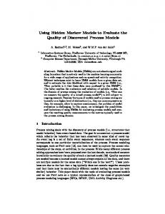
Apr 28, 1991 - âplace 111 112 27 109 114. EY(L,SH) âlation 111 112 27. 68. 21. (a) triphone example. B1. B2. M. E1. E2. AE(K,S) âcastle 113 16 76 105 122.
Shared-Distribution Hidden Markov Models for Speech Recognition Mei-Yuh Hwang Xuedong Huang April 28, 1991 CMU-CS-91-124
School of Computer Science Carnegie Mellon University Pittsburgh, PA 15213
Abstract Parameter sharing plays an important role in statistical modeling since training data are usually limited. On the one hand, we would like to use models that are as detailed as possible. On the other hand, with models too detailed, we can no longer reliably estimate the parameters. Triphone generalization may force two models to be merged together when only parts of the model output distributions are similar, while the rest of the output distributions are different. This problem can be avoided if clustering is carried out at the distribution level. In this paper, a shared-distribution model is proposed to replace generalized triphone models for speaker-independent continuous speech recognition. Here, output distributions in the hidden Markov model are shared with each other if they exhibit acoustic similarity. In addition to detailed representation, it also gives us the freedom to use a large number of states for each phonetic model. Although an increase in the number of states will increase the total number of free parameters, with distribution sharing we can essentially eliminate those redundant states and have the luxury to maintain necessary ones. By using the shared-distribution model, the error rate on the DARPA Resource Management task has been reduced by 20% in comparison with the baseline SPHINX system.
This research was sponsored by the Defense Advanced Research Projects Agency under Contract N00039-91-C0158. The views and conclusions contained in this document are those of the authors and should not be interpreted as representing the official policies, either expressed or implied, of the U.S. Government.
Keywords: Speech recognition, hidden Markov models
Contents 1. Introduction
1
2. The Improved SPHINX System
3
::::::::::::::::::::::::::::::::: Training : : : : : : : : : : : : : : : : : : : : : : : : : : : : : : : : : : : : : : Recognition : : : : : : : : : : : : : : : : : : : : : : : : : : : : : : : : : : : :
2.1. Signal Processing
3
2.2.
3
2.3.
3. Distribution Sharing
:::::::::::::::::: Incorporation of Shared Distributions into SPHINX : 3.2.1. Model Topology : : : : : : : : : : : : : : : 3.2.2. Training and Interpolation : : : : : : : : : : Model-Level and Distribution-Level Clusters : : : :
3.1. Sharing Algorithm 3.2.
3.3.
5 7
: : : : :
: : : : :
: : : : :
: : : : :
: : : : :
: : : : :
: : : : :
: : : : :
: : : : :
: : : : :
: : : : :
: : : : :
: : : : :
: : : : :
: : : : :
4. Performance and Discussions
:::::::::::::::::::::::::::::::: Recognition Performance : : : : : : : : : : : : : : : : : : : : : : : : : : : : :
7 10 10 10 12 16
4.1. Evaluation Database
16
4.2.
16
5. Conclusion and Future Work
19
1. Introduction In speech recognition, hidden Markov models (HMMs) have been successfully used to model various acoustic phenomena [13, 21, 27, 4, 17, 24, 18]. In these systems, each HMM is responsible for representing a specific unit of speech, such as a phoneme or a word. An HMM consists of several states and transition arcs between these states. Associated with each state i is an output distribution, bi (:), representing a distinct acoustic event in that unit of speech.1 State transition probabilities aij ’s specify time-varying properties related to different acoustic events. The output probability can be a mixture of continuous probability density functions [15, 31], or a discrete or semi-continuous output probability distribution [2, 21, 10]. The forward-backward algorithm [2] is generally used to iteratively reestimate both output and transition probabilities, and the Viterbi beam search algorithm [36, 32] is used during recognition to find out the most likely word sequence. Interested readers are referred to [19, 30, 9, 37] for more detailed treatments on HMMs for speech recognition. To improve the structure of the stochastic model of speech, the complexity or dimensionality of the model usually needs to be increased; this leads to the increased effective number of degreesof-freedom in the models. For large vocabulary speech recognition, hidden Markov modeling of words becomes more difficult because of the many repetitions needed to train a single word HMM. Instead, subword units like context-dependent phonetic models are introduced [1, 34, 20] as they are both consistent and trainable units. A triphone is a phone that takes into consideration its left and right phonetic contexts. Triphone models are typically poorly trained because there are so many of them. For example, there are approximately 7500 context-dependent triphones [32, 11] in the DARPA Resource Management (RM) task [29]. If each triphone is represented by a discrete HMM, there will be several millions of parameters to be estimated. To estimate the increased number of free parameters, more training data are generally needed. Conversely, faced with a limited amount of training data, the advantage of improved structure of the stochastic model may not be realized since these free parameters may not be reliably estimated. Thus, one of the most important issues in designing an HMM-based system is how to estimate a huge amount of parameters with only limited training data. Because of the dilemma between detailed model structure and available training data, we must resort to a way of smoothing or reducing free parameters. To smooth parameters, deleted interpolation [14] or heuristic interpolation [34, 32, 3] has been successfully employed to smooth those less well-trained parameters with relative well-trained, but less detailed parameters. The interpolation weights can be determined according to the ability of predicting unseen data [14], or a function of training tokens [33]. For example, parameters of triphone models can be interpolated with parameters of diphone or context-independent phoneme models [34, 20], coocurrence matrices [34, 32], or several layers of intermediate clustered phonetic models constructed by a decision tree [23, 6]. Alternatively, to reduce the amount of free parameters, techniques based on parameter sharing have also been applied successfully in many speech recognition systems. Generalizedtriphone models [20] group similar triphones together when they are poorly trained or when they are close to each other based on an information-theoretic distance measure. Similar approaches based on the number of training tokens are also used in [18, 24]. Another parameter-sharing 1
Output distributions may also be associated with arcs instead of states.
1
example is the semi-continuous (tied-mixture) HMM (SCHMM) [9]. SCHMMs make different continuous probability density functions shared across different phonetic models. In comparison with the discrete HMM, SCHMMs use multiple codewords instead of the best codeword in vector quantization (VQ), which leads to relative well trained parameter sets. In the SPHINX system, generalized triphones [20] are used to merge similar triphones together in order to reduce the amount of parameters, However, clustering at the HMM level may not provide us with very accurate models. This is because clustering two entire models may force output distributions with quite different shapes to be merged together when only parts of the models actually exhibit close resemblance. Shared-distribution models have been successfully employed for speaker-adaptive speech recognition where adaptive distributions are shared across different phonetic models [7]. In this paper, we propose an approach that makes output distributions or HMM states shared across different phonetic models for speaker-independent continuous speech recognition. Unlike model-level clustering, distribution-level clustering merges two distributions only if these distributions themselves exhibit certain acoustic similarity. In a similar manner as the SCHMM where continuous probability density functions are shared across different phonetic models, our new approach shares HMM output distributions across different phonetic models. Shared-distribution models not only provide us with a more accurate representation but also gives us the freedom to increase the number of states in each HMM. It is true that an increase in the number of states for each HMM will result in an increased number of parameters. However, armed with distribution sharing, we can essentially eliminate those redundant states for some phonetic models and have the luxury to maintain more states for others. As long as the number of states in an HMM and the total number of shared distributions are properly determined, we can achieve both detailed and robust modeling of speech signals. The proposed method thus provides us with a general way to reduce the number of free parameters. Moreover, the same principle can be applied to either discrete, continuous, or semi-continuous HMMs. To evaluate the proposed approach, we choose the improved SPHINX speech recognition system [8] as the baseline system. The improved version of SPHINX incorporated four codebooks including both first-order and second-order dynamic features. The discrete HMMs were replaced with the sex-dependent SCHMMs. The improved system reduced the error rate of the original SPHINX system significantly [8], and had the lowest recognition error rate in the June 1990 DARPA Resource Management (RM) evaluation [26]. In this study, we modified the basic HMM topology of the SPHINX system with an increased number of distributions for each model. An information-theoretic distortion measure was used to cluster distributions across different phonetic models. We will demonstrate that distribution-level clustering indeed provides us with better representation. For the 997-word, RM, speaker-independent, continuous speech recognition task, the error rate was further reduced by 20% in comparison with the improved baseline SPHINX system. The organization of this paper is as follows. We will first review the improved SPHINX baseline system. In Section 3, the algorithm on distribution clustering and its foundations are introduced. We will also discuss practical issues and clustering examples. Section 4 includes experimental evaluation of the proposed approach with the RM task. Our conclusion and future work direction are reported in the last section.
2
2. The Improved SPHINX System SPHINX is a large vocabulary, speaker-independent, continuous speech recognition system developed at Carnegie-Mellon University [21]. Recently, the error rate of the SPHINX system was reduced by more than 50% with between-word coarticulation modeling [12], high-order dynamics [8], and sex-dependent SCHMMs [8]. This section will review the improved SPHINX system, which will be used as our benchmark system in this study.
2.1.
Signal Processing
The input speech signal is sampled at 16 kHz with a pre-emphasized filter, 1 ? 0:9Z ?1 . Hamming window with a width of 20 msec is applied to speech signal every 10 msec. The 32-order LPC analysis is followed to compute the 12-order cepstral coefficients. Bilinear transformation of cepstral coefficients is employed to approximate mel-scale representation. In addition, relative power energy is also computed together with cepstral coefficients. Speech features used in the improved SPHINX system include: 1. LPC cepstral coefficients (dimension 12) 2. 40-msec and 80-msec differenced LPC cepstral coefficients (dimension 24)
4cep(t) = cep(t + 2) ? cep(t ? 2) 4cep0(t) = cep(t + 4) ? cep(t ? 4) 3. second-order differenced cepstrum (dimension 12)
44cep(t) = 4cep(t + 1) ? 4cep(t ? 1) 4. power, 40-msec differenced power, second-order differenced power (dimension 3)
4power(t) = power(t + 2) ? power(t ? 2) 44power(t) = 4power(t + 1) ? 4power(t ? 1) These features are vector quantized into four independent codebooks by the Linde-Buzo-Gray algorithm [22], each of which has 256 entries.
2.2.
Training
The phonetic HMM topology is shown in Figure 1. There are three output distributions associated with the arcs for each HMM. They are labeled as Beginning, Middle, and Ending as illustrated in the figure. 3
B
B
M
E
E
M
B
initial
final
M
B
E M B
Figure 1: The HMM topology used in SPHINX. Training procedures are based on the forward-backward algorithm. Word models are formed by concatenating phonetic models; sentence models by concatenating word models. Forty-eight context-independent discrete phonetic models are initially estimated from the uniform distribution. Deleted interpolation [14] is used to smooth estimated parameters with the uniform distribution. There are 7549 triphone models in the DARPA RM task when both within-word and betweenword triphones are considered. Because of memory limitation, it is impossible to estimate all these triphone models. Therefore, for both the context-independent and the context-dependent model at this stage, we used only one codebook, where each codeword consists of the cepstral coefficients, 40-msec differenced cepstrum, power and 40-msec differenced power. We first started with the one-codebook system, and 7549 discrete models are estimated. The generalized-triphone clustering procedure [20] is then applied to reduce the number of models from 7549 to 1100. Here, the goal is to cluster similar triphones together such that these model parameters could be well trained. For example, EY(L,S) (which stands for the phoneme EY with immediate left context L and right context S, like –place) and EY(L,SH) (such as –lation) are merged together. In such a clustering approach, all the distributions in EY(L,S) are merged with all the distributions in EY(L,SH) respectively. As we will see in Section 3.3, clustering at the model level may merge quite different-shaped distributions together, like the the rear parts of EY(L,S) and EY(L,SH). Based on generalized triphone clusters, we first estimate 48 context-independent, four-codebook discrete models with the uniform distribution. With these context-independent models, we then estimate the 1100 generalized SCHMMs [8]. SCHMMs assume that each codeword k of a VQ codebook is represented by a continuous probability density function fk (x), where x is the acoustic vector. The discrete output distribution bi (k ) is replaced with the semi-continuous function Bi (x):
Bi ( x ) =
L X
fk (x)bi(k) k=1 where L is the codebook size. In practice, 2 to 8 most significant fk (x)’s are adequate. We assume that each fk (x) is a Gaussian density function with mean k and diagonal covariance k . Means and covariance matrices are reestimated according to the following formula [9]:
�
P P � (i;k ) x �k = P t P i P t � (i; kt) t
i
4
k
t
�
�k = �
P P t
i
�Pt(i;k )(xt ? �k )t P ) (Pxt ?��(ki;k ) t i k t
where t (i;k ) is the probability that at time t, VQ symbol k is emitted at state i. Because of substantial difference between male and female speakers, sex-dependent SCHMMs are employed to enhance the performance. To summarize, the configuration of the improved SPHINX system has:
� � � 2.3.
four codebooks, 1100 generalized between-word and within-word triphone models, sex-dependent SCHMMs.
Recognition
In recognition, a language network is pre-compiled to represent the search space. Figure 2 shows a part of the language network which illustrates the connections of what’s ! a and what’s ! the. Connection through SIL (silence) represents less coarticulated speech at the word boundary, while those such as TS(36) ! DH(10), TS(9) ! AX(4), and TS(9) ! AX(5) attempt to capture the strong between-word coarticulation in fluent speech. Here, generalized triphone TS(36) represents the cluster containing TS(AH,DH)e.2 As will be described in this paper, when shared distributions are used, TS(36) will be restored to be TS(AH,DH)e since no two triphones will be completely merged, albeit parts of their parameters may be shared with each other. For each input utterance, the Viterbi beam search algorithm is used to find out the optimal state sequence in the language network. In order to use sex-dependent SCHMMs, codebook-based sex classification [7, 35] is carried out before recognition starts. Experiments show that the error rate of sex-classification is below 1%. Based on sex classification, only the corresponding sex-dependent SCHMMs are activated for the Viterbi search. 2
The suffix e means this triphone appears at the end of a word.
5
a
SIL
AX(4) AX(5)
what’s
AX(28) AX(41)
W(20)
TS(1) AH(7)
TS(9) TS(36) the
DH(2) DH(10)
Figure 2: The network used in Viterbi beam search.
6
AX(3)
3. Distribution Sharing Although triphone generalization provides us with a way to reduce the number of free parameters, it nevertheless introduces many inaccurate models since two quite different output distributions may be forced to be combined whenever two models are clustered. In contrast, clustering at the distribution level could avoid this problem and achieve the same goal—reduce the amount of parameters. It also provides us with the freedom to have more elaborate acoustic representation as we can use a large number of states for each HMM.
3.1.
Sharing Algorithm
In order to merge two output distributions, we need to define the distortion measure between them. There are many ways to measure the distance of two distributions/HMMs, such as distortion measures based on cross entropy [16], divergence and discrimination information [16], output string/symbol probability [5], maximum mutual information [5], chi-square measure [28], and generalized triphone distance measure [20]. All these distortion measures could provide us with reasonable clustering results. While triphone generalization clusters triphones, our goal is to cluster distributions. Thus, the major difference is the granularity of the clustered objects. Here, the distortion measure is based on the amount of information loss when two distributions/clusters are merged, which works in the same way as the one used in generalized triphone clustering. cluster
cluster
a1/A
b1/B
a2/A
b2/B
aL/A
bL/B
merged cluster
(a1+b1)/(A+B) (a2+b2)/(A+B)
(aL+bL)/(A+B)
Figure 3: Clustering of two distributions. To elaborate, suppose there are two distributions � and , each with L entries. The occurrence 7
counts for each entry in � and are denoted as a1 ;a2 ; :::;aL , and b1; b2 ; :::;bL respectively. Let PL a = A; PL b = B . The entropy for distribution � and can be computed as follows: i=1 i i=1 i
H� = ?
L a X i A i=1
log
ai A
H = ?
L b X i i=1 B
log
bi B
When two distributions are merged, the new count for the resulting distribution is the summation of the two merged distributions. Therefore, the entropy for the resulting distribution is:
H=?
L a +b X i i A + B i=1
log
ai + bi A+B
The entropy (uncertainty) increase, weighted by counts, due to merging two distributions can be computed as:
(�; ) = (A + B )H ? AH� ? BH i h � � = ? P a log a +bi ? log a i i
? Pi bi
i
i
h
�
A+B
log aAi++Bbi
A
�
?
log bBi
i
� � h� � � �i = ? A Pi aA log aA++Bb = aA � � h� � � �i ? B P b log a +b = b i
i Bi
It can be verified that ln(x) it can be derived that X
i
i
i
i
i
B
i
A+B
� x ? 1 with equality if and only if x = 1. Given this inequality,
xi log xyi �
X
X
yi i i i i with equality if and only if xi = yi , 8i. Therefore, the uncertainty increase is always greater than P P bi = P ai+bi = 1, with zero if and only if a =A = b =B , 8i, that or equal to zero since i aAi = i B i i i A+B is, when two probability distributions are exactly the same. The most similar pair of clusters is defined to be the pair that, when merged, gives the least uncertainty increase. Weighting entropy by the occurrence count can also take into account how well a distribution is trained. For those distributions that appear infrequently, they will be merged first in comparison with those well trained ones. This makes each shared distribution more trainable. if
0
xi =
Using such a distortion measure, the clustering algorithm can be described as follows:
8
1. All HMMs are first estimated. 2. Initially, every distribution of all HMMs is created as a cluster. 3. Find the most similar pair of clusters and merge them together. 4. For each pair of clusters, consider moving every element from one to the other: (a) move the element if the resulting configuration is an improvement; (b) repeat until no such moves are left. 5. Go to step 3 unless some convergence criterion is met.
Without step 4, this would just be a greedy algorithm, where every merge could not be undone. Step 4 is a heuristic optimization that attempts to improve the clustering procedure by allowing elements to be moved from one cluster to another. In step 4(a), a new configuration is considered to be an improvement if its grand weighted entropy is less than that of the existing one. The grand weighted entropy is computed as the sum of the weighted entropies of all the clusters in the configuration. To reduce computational complexity at step 4, step 4(b) can be terminated prematurely when the number of movements are over a predefined threshold, or when a minimum improvement fails. In addition, when an element is to be moved, recomputation of the entropies for the two changed clusters is also expensive. Therefore, unlikely moves should not be considered. To achieve this goal, poorly trained distributions are not worthy of reconfiguration. Besides, we can utilize the uncertainty increase matrix for all the distribution pairs, (d1 ; d2 ), to decide unlikely moves. The uncertainty increase matrix is computed once and for all at the first time of step 3. While considering whether to move distribution d from cluster 1 to cluster 2, we first compare the average uncertainty increases for d when it is in cluster 1 and in cluster 2. The average uncertainty increase for distribution d can be easily derived from the uncertainty increase matrix as follows:
0
(d) = @
1 � ?
(d; i)A = size(cluster 1 ) ? 1 i6=d; i2cluster 1 0 1 X
0(d) = @
(d; i)A =size(cluster 2 ) X
i2cluster 2 0 Only if the ratio of (d)= (d) is less than a predefined threshold, do we compute the grand weighted entropy of the new configuration to see if moving d will lead to an improvement.
The convergence criterion in step 5 could be the total number of clusters left or a maximum ratio of the new grand weighted entropy over the previous one, and the like. The clustering algorithm provides an ideal means for finding equilibrium between trainability and sensitivity. Given a fixed amount of training data, it is possible to find the largest number of trainable distributions or the smallest number of sensitive distributions. 9
3.2. 3.2.1.
Incorporation of Shared Distributions into SPHINX Model Topology
With distribution sharing, we have the freedom to use more states and distributions for each phonetic HMM in order to have more detailed acoustic representation. When extra distributions are used for each HMM, our clustering procedure will automatically squeeze those redundant distributions and keep those necessary ones. However, the number of states should not be too large because we have to obtain a set of reliable HMMs for the clustering algorithm.
initial
B1
B1
E1
M
B2
B1
B2
E2
E1
M
M
B2
E2
final
E1
Figure 4: The new topology used in the shared-distribution model. The baseline SPHINX system has three distributions for each HMM. We increase the number of distributions for each model by about 60%. The new topology is shown in Figure 4. It is a left-to-right Bakis HMM with five distributions. No output distribution is associated with the final state in order to facilitate implementation. This topology will be used for subsequent experiments conducted in this paper.
3.2.2.
Training and Interpolation
As described in Section 2.2, we first estimated the one-codebook based, 48 context-independent and 7549 context-dependent discrete models using the topology shown in Figure 4. This gave us the estimates needed for the clustering algorithm, where the distributions of the 7549 5-distribution discrete HMMs need to be clustered. After clustering is done, the next step is to train 4-codebook models. Context-independent discrete models are estimated based on the uniform distribution. Here, no shared distributions are employed since these context-independent models have sufficient training data. Then contextdependent SCHMMs with shared distributions are estimated. To apply the forward-backward algorithm for the shared-distribution model, parameter counts for shared distributions need to be accumulated before Baum-Welch reestimation. In the same manner as the SCHMM, parametersharing will not affect the maximum likelihood estimation criterion [9]. The Q-function can be modified to prove this [9]. To initialize each shared distribution for the 7549 context-dependent models, one component distribution is randomly chosen from the corresponding distribution cluster. The context-independent 10
counterpart is used as the initial shared distribution. For example, Table 1 shows all the members in the 94th D shared distribution when these 7549 � 5 distributions are merged into 4500 clusters. If by chance, distribution B2 of context-dependent model D(S,AE) is selected, the B2 distribution from the context-independent model D will be copied as the initial value for the 94th D shared distribution. triphone distribution D(S,AA) B1 D(S,AO) B1 ; B2 D(S,EY) B1 D(S,R)b B1 ; B2 D(Z,EY) B1
triphone distribution D(CH,AA)b B1 D(S,EH) B1 D(S,IY) B1 D(TS,ER)b B1
triphone distribution D(S,AE) B1 ; B2 D(S,ER)b B1 D(S,IY)b B1 D(Z,AX)b B1
Table 1: Members of the 94th D shared distribution when 4500 clusters are left. We experimented with 3500, 4500, and 5500 shared distributions for these 7549 models. As will be discussed in Section 4, 4500 distributions produced the best recognition accuracy. In these experiments, no matter how many distributions are used, HMM transitions are never shared with each other. Therefore, there are 7549 � 14 transition probabilities (v.s. 1100 � 12 in 1100 generalized triphones).
from cxt-indep model
EY B1
B2
E1
M
E2
from last iter. of F/B algorithm
EY(L,S) 111
112
27
109
114
interpolated furthermore with uniforms interpolated-
smoothed parameters
EY(L,S)
Figure 5: Expansion from shared distributions. Context-dependent models need interpolation to make them have better generalization capability. To start interpolation, we first expand the shared distributions (Figure 5), assuming the clustering of EY(L,S)’s distributions is given in Table 3(a) in Section 3.3. Every unshared distribution of a triphone is copied from the shared distribution to which it belongs. These unshared distributions are interpolated with the corresponding context-independent model and the uniform 11
distribution. Thus, after interpolation, there may be several interpolated versions for the same shared distribution. For example, from Table 1, there will be 16 interpolated distributions for the 94th D cluster, respectively from the B1 distribution of interpolated D(S,AA), B1 and B2 of interpolated D(S,AO), and so on. To maintain the sharing structure, the counts of the interpolated distributions that originate from the same shared-distribution cluster are subsequently averaged to obtain final estimates. In addition to distribution interpolation, transitions of context-dependent models are also interpolated with those of context-independent ones.
3.3.
Model-Level and Distribution-Level Clusters
Based on RM training data, Table 2 shows the number of shared distributions for each phonetic model when 7549 � 5 distributions are merged to 4500 clustered distributions. The number of triphones for each phone is also included in the table. In this experiment, two distributions are merged only if they represent the same context-independent phonetic model. It is also possible to merge distributions across different phonetic models, albeit experiments for speaker adaptation indicated this did not make any significant difference [7]. phone AE EH IH IY UH AH AX IX AA AO UW AW AY EY OW OY
triphone# cluster# 138 127 211 211 148 133 309 162 12 13 52 58 431 247 119 144 126 108 67 52 119 102 27 31 80 58 178 129 161 100 2 6
phone L R W Y EN ER M N NG CH JH B D DH G K
triphone# cluster# 327 178 251 171 124 67 59 35 10 12 250 147 252 125 468 250 43 43 89 44 95 35 141 74 179 109 71 60 97 54 249 126
phone P T F S SH TH V Z HH SIL DD PD TD KD DX TS
triphone# cluster# 171 82 200 108 237 91 462 188 84 45 128 54 179 110 385 142 109 50 1 unshared 194 94 34 16 269 167 75 43 40 51 97 48
Table 2: The number of triphones and shared distributions for each context-independent phone. There are a total of 4500 shared distributions and 7549 triphones. To understand the difference between model-level and distribution-level clustering, clusters generated by both techniques are carefully examined. Here, we compared 1100 3-distribution generalized triphone models and 4500 shared distributions clustered from the 5-distribution model. Both approaches combine similar triphone distributions as well as less well trained distributions together. However, distribution-level clustering provides us with more flexibility. 12
Table 3 illustrates several typical distribution clusters generated by these two clustering algorithms. Let P(L,R) denote phoneme P with left context L and right context R. Let P(L,R)b denote the triphone that appears at the beginning of the word, P(L,R)e denote the last triphone of the word, and P(L,R)s denote exclusively for single-phone word. Triphones without any suffix occur only within a word. Triphones in the same subtable are in the same generalized triphone cluster. Indices in the table are the labeling within all the shared-distribution clusters that represent the same context-independent phone. In Table 3(a), it is reasonable to see that triphone EY(L,S) and EY(L,SH) are in the same generalized triphone cluster as they have the same left-context. Unfortunately, model-level clustering must ignore the differences of right-contexts due to the fact that the front parts of these two models are very similar. On the other hand, clustering at distribution-level can keep the difference apart despite that those resemblance parts are merged. Thus, these two triphones are represented by seven distributions (111, 112, 27, 109, 114, 68, 21) in comparison with only five distributions if both EY(L,S) and EY(L,SH) have five distributions and are merged by the generalized triphone approach. This clearly demonstrates that the shared-distribution models have more detailed representation in comparison with the generalized triphone models. Forcing models (multiple distributions) to be shared with each other will not be as accurate as forcing sub-model units (single distribution) to be shared with each other. Table 3(b) is illustrates again that distributions in similar contexts are merged and distinctive ones retained. There are cases that distributions of two triphones are not shared at all, even though they represent similar triphones. For example, both the left and right contexts of the two triphones in Table 3(c) are the same. The only difference is their locations — one of them appears within a word like threat and the other appears at the beginning of a word like at in the context things are at somewhere. This may be partly due to dramatic acoustic transition changes at the word boundary in fluent speech, and partly because of the fact that the word-boundary triphones do not occur as frequently as those within-word triphones. From Table 3(c), we also see that the first three distributions of EH(R,TD) are combined together. This indicates three distributions are sufficient to model its acoustic variations. Thus, the shared-distribution clustering procedure is able to squeeze redundant distributions inside an HMM elegantly. Despite the enhanced capability of shared-distribution models, we also observed some unexpected clustering results. One example is illustrated in Table 3(d). We can see that the first four distributions of D(Z,EY) and D(S,EY) are forced to be grouped together even though their leftcontexts are different. The reason for such merging could be due to less well-trained distributions and the fact that the realization of a phoneme may be affected not only by its immediate contexts but also far-away contexts. In addition to investigate how different triphone models are organized, we also examined what each shared distribution consists of. Table 1 from the previous subsection and Table 4 list all of the members for the 94th D and the 27th EY shared distributions. These two tables show us that the 94th D shared distribution consists of the 1st and 2nd ( B1 and B2 ) distributions of several triphone models in different contexts, and the 27th EY shared distribution consists of the 3rd ( M ) distribution of several triphone models. It is interesting that the k -th distribution of one triphone model is usually merged first with the k -th distribution of other triphone models. Thus, distributions that are in the same cluster are mostly from the the same k -th distribution of different models. Moreover, 13
triphone example EY(L,S) –place EY(L,SH) –lation
B 1 B2 M 111 112 111 112
E1
E2
27 109 27 68
114 21
(a) triphone example B1 AE(K,S) –castle 113 AE(K,Z) casrep– 113
B2 M 16 16
76 76
E1 E2 105 122 53 52
(b)
B1 B2 M E1 E2
triphone example EH(R,TD) threat EH(R,TD)b are at
65 63
65 185
65 63
61 113 64 207
(c) triphone D(Z,EY) D(S,EY)
B1 B2 M
example Tuesday state
94 105 94 105
95 95
E1 E2 103 103
96 87
(d)
Table 3: Shared distributions of several triphones; triphones in the same subtable are in the same generalized triphone cluster.
triphone distribution EY(M,K) M EY(L,IH)e M EY(L,P)e M EY(L,S) M
triphone distribution EY(L,DX) M EY(L,SH) M EY(L,B)e M
Table 4: Members of the 27th EY shared distribution when 4500 clusters are left.
14
the first two distributions are never merged with the last two distributions. When we reduced the total number of distributions to 4500, the average number of unique distributions in each triphone model is 4:655. This shows that most of the triphone models keep 5 unique distributions. As each triphone tends to keep more states, the original 3-distribution based SPHINX system has obviously insufficient distributions. To justify this, DARPA RM task will be used to evaluate the proposed method in the following section.
15
4. Performance and Discussions In order to create highly versatile and useful systems, research on large vocabulary, speakerindependent, continuous speech recognition is particularly important. This study is intended to improve acoustic-modeling performance using the shared-distribution models.
4.1.
Evaluation Database
The task, DARPA’s resource management, which is designed for inquiry of naval resources [29], was used to evaluate the shared-distribution models in comparison with the improved baseline SPHINX system [8]. At the lexical level, the 997-word resource management task is very complex. There are many confusing pairs, such as what and what’s, the and a, four and fourth, any and many, and many others. Most of the proper nouns can appear in singular, plural, and possessive forms. On the other hand, at the grammatical level, the task is not a very difficult one because the sentences are generated from a set of 900 sentence templates which resemble realistic questions in a database query system. The most obvious and correct way to model the RM task language is to use a finite state language that generates the same set of sentences as those 900 templates. As the perplexity of such a grammar is too low (about 9) to evaluate the acoustic part of a speech recognition system, the word pair grammar, which can generate all sentences including the 900 sentence templates and some illegal sentences, is used here. The word pair grammar specifies only the list of words that can legally follow any given word, which can be extracted from the 900 sentence templates. Each template is a network of tags, or categories of words. Given these templates, the list of tags that can follow any given tag can be easily determined. From this information and the list of words in each tag, a list of words that can follow any given word can then be generated. The word-pair grammar specifies 57,878 word pairs, versus 997 � 997 = 994,009 possible word pairs. This grammar has a test-set perplexity of about 60. During recognition, each word HMM can be followed only by those word HMMs allowed by the word-pair grammar. The transition probability between a given word HMM to a following word HMM is 1=k , where k is the number of words that can follow the given word. The speech database used for the development of SPHINX consists of 3990 training sentences from 105 speakers and 600 test sentences (used in February and October 1989 evaluations) from 20 new speakers.
4.2.
Recognition Performance
We replaced generalized triphone models with shared-distribution models in SPHINX. The new technique was evaluated with the RM task. Varying the total number of shared distributions from 3500 to 5500, a series of experiments 16
system error rate baseline SPHINX 4.7% 3500 shared dists 4.2% 4500 shared dists 3.8% 5500 shared dists 4.1%
error reduction — 11% 20% 13%
Table 5: Error rates with the word-pair grammar.
system error rate baseline SPHINX 19.5% 4500 shared dists 17.9%
error reduction — 8%
Table 6: Error rates with no-grammar.
were conducted in comparison with the baseline SPHINX system. The error rates of different distribution sizes on the test set are shown in Table 5 and Table 6 for the word-pair grammar and no-grammar respectively. Word errors include substitutions, deletions, and insertions. The error reduction rates compared with the baseline SPHINX system are also computed. From these experiments, we can see that shared-distribution models outperformed generalized triphone models. When 1100 generalized triphone models are used, there are 3300 distributions in total. With about the same amount of parameters, 3500 shared distributions reduced the error rate by 11%. This demonstrated that shared-distribution models have more accurate representation since combination of two distributions are not enforced by other distributions. When we increased the total number of shared distributions from 3500 to 4500, the error rate was reduced by about 20% in comparison with the baseline SPHINX. Further increase in the total number of shared distributions to 5500 did not give us any more improvement, as they may not have been well trained. When no grammar is used, the error reduction is not as high as the word-pair grammar case. This is partly because the duration we used was estimated by using within-word generalized triphone models, and partly because the no-grammar system requires less smoothed models. In these experiments, the transition probabilities have been deemphasized. Our experiments show that it is not very sensitive, especially when multiple codebooks are used. In fact, we found that uniform transition probabilities yield only slightly worse results. Since we used more states in these experiments in comparison with the baseline SPHINX, our improvements might not come from shared-distribution models, but from the increased number of states within each triphone. To clarify, we tested 1100 generalized triphone models by increasing the number of distributions to five for each model. The results are shown in Table 7. The error rate was 4.6% for the same test set, which is about the same as the original baseline system. As there are 5500 distributions in 5-distribution based generalized triphone system, we include 17
shared-distribution models with the same number of distributions in the table. Once again, the shared-distribution model outperformed the generalized triphone model. This demonstrates that distribution sharing does contribute to our improvements.
error rate
3-dist 1100 5-dist 1100 5500 generalized triphones generalized triphones shared dists. 4.7% 4.6% 4.1%
Table 7: Error rates using generalized triphones and shared distributions. The shared-distribution model has been incorporated into SPHINX system and was evaluated with the DARPA February-1991 test set. Under the same training and testing conditions, results reported from different sites are shown in Table 8. Our new SPHINX system had the lowest recognition error rate among the the top 5 systems evaluated in February 1991 [25].
word-pair grammar no grammar
AT&T 5.2% 19.8%
BBN CMU 3.8% 3.6% 18.8% 17.0%
MIT-LL 4.4% 19.7%
SRI 4.8% 17.6%
Table 8: Official RM evaluation conducted in February 1991.
18
5. Conclusion and Future Work Each distribution in an HMM describes certain acoustic event. Triphone generalization may force two models to be merged together when only parts of model output distributions are similar. Combination of those quite different distributions will lead to degraded representation as different acoustic events are blended. In this paper, a novel method for parameter reduction is employed to have distribution shared across different phonetic HMMs. Classification of acoustic events at distribution level provides us with an elegant way toward more detailed modeling. In addition to detailed representation over generalized triphone, it also gives us the freedom to use more states for each phonetic model. The principle of shared distributions proposed in this paper can be applied to either discrete, continuous, or semi-continuous HMMs. This method also provides us with a way to learn the topology of HMMs. When shared distributions occur inside a model, this indicates redundant structure in the model topology. By using more complicated model topology and shared-distribution modeling, we could prune away redundant states while keeping those necessary ones. With the DARPA Resource Management task, we demonstrated that clustering at distributionlevel is superior to conventional techniques. The error rate of the baseline SPHINX system was reduced by 20%. In this study, several issues remain to be further explored:
� � �
What is the optimal number of distributions in the HMM topology? What is the optimal total number of shared distributions? What is the optimal distortion measure for distribution clustering?
In order to reliably estimate model parameters with fixed amount of training data, we have to trade off the number of distributions within each HMM and the number of distributions within each shared cluster. In our experiments, 5 states per HMM with 4500 distributions in total means 5 � 7549=4500 = 8:39 distributions per cluster on average. Increasing the number of states to 10 for each HMM and maintaining the ratio of 8.39 distributions per cluster will result in 9000 shared distributions. It is unlikely that they can be reliably trained. On the other hand, if we reduce the number of distributions down to 4500, we will on average have 16.78 distributions per cluster. Will this make each cluster blurred? Alternatively, we can use 3 states per HMM and have 6000 shared distributions, we would have 3.77 distributions per cluster. Will 3 states be sufficient to model these phonemes? All these problems need to be further addressed.
Acknowledgments The authors would like to thank Raj Reddy for his encouragement and support. The authors are also grateful to Kai-Fu Lee and Hsiao-Wuen Hon for their help and comments. 19
References [1] Bahl, L. R., Bakis, R., Cohen, P. S., Cole, A. G., Jelinek, F., Lewis, B. L., and Mercer, R. L. Further Results on the Recognition of a Continuously Read Natural Corpus. in: IEEE International Conference on Acoustics, Speech, and Signal Processing. 1980. [2] Bahl, L. R., Jelinek, F., and Mercer, R. A Maximum Likelihood Approach to Continuous Speech Recognition. IEEE Transactions on Pattern Analysis and Machine Intelligence, vol. PAMI-5 (1983), pp. 179–190. [3] Chow, Y., Dunham, M., Kimball, O., Krasner, M., Kubala, G., Makhoul, J., Roucos, S., and Schwartz, R. BYBLOS: The BBN Continuous Speech Recognition System. in: IEEE International Conference on Acoustics, Speech, and Signal Processing. 1987, pp. 89–92. [4] Doddington, G. Phonetically Sensitive Discriminants for Improved Speech Recognition. in: IEEE International Conference on Acoustics, Speech, and Signal Processing. 1989, pp. 556–559. [5] D’Orta, P., Ferretti, M., and Scarci, S. Phoneme Classification for Real Time Speech Recognition of Italian. in: IEEE International Conference on Acoustics, Speech, and Signal Processing. 1987, pp. 81–84. [6] Hon, H. and Lee, K. Recent Progress in Robust Vocabulary-Independent Speech Recognition. in: DARPA Speech and Language Workshop. Morgan Kaufmann Publishers, San Mateo, CA, 1991. [7] Huang, X. A Study on Speaker-Adaptive Speech Recognition. in: DARPA Speech and Language Workshop. Morgan Kaufmann Publishers, San Mateo, CA, 1991. [8] Huang, X., Alleva, F., Hayamizu, S., Hon, H., Hwang, M., and Lee, K. Improved Hidden Markov Modeling for Speaker-Independent Continuous Speech Recognition. in: DARPA Speech and Language Workshop. Morgan Kaufmann Publishers, San Mateo, CA, 1990, pp. 327–331. [9] Huang, X., Ariki, Y., and Jack, M. Hidden Markov Models for Speech Recognition. Edinburgh University Press, Edinburgh, U.K., 1990. [10] Huang, X. and Jack, M. Semi-Continuous Hidden Markov Models for Speech Signals. Computer Speech and Language, vol. 3 (1989), pp. 239–252. [11] Hwang, M., Hon, H., and Lee, K. Between-Word Coarticulation Modeling for Continuous Speech Recognition. Technical Report, Carnegie Mellon University, April 1989. [12] Hwang, M., Hon, H., and Lee, K. Modeling Between-Word Coarticulation in Continuous Speech Recognition. in: Proceedings of Eurospeech. 1989, pp. 5–8. [13] Jelinek, F. Continuous Speech Recognition by Statistical Methods. Proceedings of the IEEE, vol. 64 (1976), pp. 532–556.
20
[14] Jelinek, F. and Mercer, R. Interpolated Estimation of Markov Source Parameters from Sparse Data. in: Pattern Recognition in Practice, edited by E. Gelsema and L. Kanal. North-Holland Publishing Company, Amsterdam, the Netherlands, 1980, pp. 381–397. [15] Juang, B. H. and Rabiner, L. R. Mixture Autoregressive Hidden Markov Models for Speech Signals. IEEE Transactions on Acoustics, Speech, and Signal Processing, vol. ASSP-33 (1985), pp. 1404–13. [16] Juang, B. and Rabiner, L. A Probabilistic Distance Measure for Hidden Markov Models. The Bell System Technical Journal, vol. 64 (1985), pp. 391–408. [17] Kubala, F. and Schwartz, R. A New Paradigm for Speaker-Independent Training and Speaker Adaptation. in: DARPA Speech and Language Workshop. Morgan Kaufmann Publishers, San Mateo, CA, 1990. [18] Lee, C., Giachin, E., Rabiner, R., L. P., and Rosenberg, A. Improved Acoustic Modeling for Continuous Speech Recognition. in: DARPA Speech and Language Workshop. Morgan Kaufmann Publishers, San Mateo, CA, 1990. [19] Lee, K. Automatic Speech Recognition: The Development of the SPHINX System. Kluwer Academic Publishers, Boston, 1989. [20] Lee, K. Context-Dependent Phonetic Hidden Markov Models for Continuous Speech Recognition. IEEE Transactions on Acoustics, Speech, and Signal Processing, April 1990, pp. 599–609. [21] Lee, K., Hon, H., and Reddy, R. An Overview of the SPHINX Speech Recognition System. IEEE Transactions on Acoustics, Speech, and Signal Processing, January 1990, pp. 35–45. [22] Linde, Y., Buzo, A., and Gray, R. An Algorithm for Vector Quantizer Design. IEEE Transactions on Communication, vol. COM-28 (1980), pp. 84–95. [23] Lucassen, J. Discovering Phonemic Baseforms: an Information Theoretic Approach. Research Report, no. RC 9833, IBM, February 1983. [24] Murveit, H., Butzberger, J., and Weintraub, M. Speech Recognition in SRI’s Resource Management and ATIS Systems. in: DARPA Speech and Language Workshop. Morgan Kaufmann Publishers, San Mateo, CA, 1991. [25] Pallett, D., Fiscus, J., and Garofolo, J. DARPA Resource Management Benchmark Test Results. in: DARPA Speech and Language Workshop. Morgan Kaufmann Publishers, San Mateo, CA, 1991. [26] Pallett, D., Fiscus, J., and Garofolo, J. DARPA Resource Management Benchmark Test Results June 1990. in: DARPA Speech and Language Workshop. Morgan Kaufmann Publishers, San Mateo, CA, 1990, pp. 298–305. [27] Paul, D. The Lincoln Robust Continuous Speech Recognizer. in: IEEE International Conference on Acoustics, Speech, and Signal Processing. 1989, pp. 449 – 452. 21
[28] Paul, D. and Martin, E. Speaker Stress-Resistant Continuous Speech Recognition. in: IEEE International Conference on Acoustics, Speech, and Signal Processing. 1988. [29] Price, P., Fisher, W., Bernstein, J., and Pallett, D. A Database for Continuous Speech Recognition in a 1000-Word Domain. in: IEEE International Conference on Acoustics, Speech, and Signal Processing. 1988, pp. 651–654. [30] Rabiner, L. A Tutorial on Hidden Markov Models and Selected Applications in Speech Recognition. IEEE Proceedings, 1989. [31] Rabiner, L., Wilpon, J., and Soong, F. High Performance Connected Digit Recognition Using Hidden Markov Models. IEEE Transactions on Acoustics, Speech, and Signal Processing, vol. 37 (1989), pp. 1214–1225. [32] Schwartz, R., Chow, Y., Kimball, O., Roucos, S., Krasner, M., and Makhoul, J. ContextDependent Modeling for Acoustic-Phonetic Recognition of Continuous Speech. in: IEEE International Conference on Acoustics, Speech, and Signal Processing. 1985, pp. 1205– 1208. [33] Schwartz, R., Kimball, O., Kubala, F., Feng, M., Chow, Y., C., B., and J., M. Robust Smoothing Methods for Discrete Hidden Markov Models. in: IEEE International Conference on Acoustics, Speech, and Signal Processing. 1989, pp. 548–551. [34] Schwartz, R. M., Chow, Y. L., Roucos, S., Krasner, M., and Makhoul, J. Improved Hidden Markov Modeling of Phonemes for Continuous Speech Recognition. in: IEEE International Conference on Acoustics, Speech, and Signal Processing. 1984. [35] Soong, F., Rosenberg, A., Rabiner, L., and Juang, B. A Vector Quantization Approach to Speaker Recognition. in: IEEE International Conference on Acoustics, Speech, and Signal Processing. 1985, pp. 387–390. [36] Viterbi, A. J. Error Bounds for Convolutional Codes and an Asymptotically Optimum Decoding Algorithm. IEEE Transactions on Information Theory, vol. IT-13 (1967), pp. 260–269. [37] Waibel, A. and Lee, K. Readings in Speech Recognition. Morgan Kaufman Publishers, San Mateo, CA, 1990.
22