SHARING SIMULATION MODELS AND TOOLS WITHIN A COLLABORATIVE RESEARCH PROJECT Andriy Levytskyy, Eugene J.H. Kerckhoffs Delft University of Technology Faculty of Information Technology and Systems Mediamatica Department Mekelweg 4, 2628 CD Delft, The Netherlands
[email protected]
KEYWORDS Collaborative simulation environment, heterogeneous models, heterogeneous tools, metadata, the Internet. ABSTRACT Our research aims at developing and building a generic collaborative environment to support a research and development process, in which heterogeneous (in formalism and format) models are being shared, reused and executed on distributed heterogeneous tools via the Internet. In this paper we briefly describe the implementation of the environment in its current state and consider the functionality of our environment with respect to sharing simulation models and tools.
1. Introduction Research and development in multidisciplinary collaborative projects is characterised by a number of particularities. The multidisciplinary teams are distributed geographically, they are free in their choice of research tools and their knowledge domains differ substantially. As the result, there exists significant variety of formats, in which the data and models are being developed by the collaborators. It also means that in order to perform any meaningful actions with such heterogeneous data formats, collaborators have to access the respective tools and have the expertise beyond their research domains to deal with technical idiosyncrasies of those tools. Our research addresses the needs for a seamless integration of various simulation tools and seamless representation and manipulation of models in different formats and formalisms. The goal of our project is a generic collaborative “different place and different/same time” environment for sharing models and simulations. The environment is intended to support running web-accessible models on distributed heterogeneous tools, as well as piping and linking simulations and other applications according to user specifications, herewith tackling semantic differences in model formalisms and in interfaces between different simulations. The final generic system is to be adjusted to
Hans Vangheluwe McGill University School of Computer Science 3480 University Street Montreal, Quebec, Canada H3A 2A7
cover any concrete situation at hand (i.e., any concrete collaborative research project with its specific research tools). In this paper we present the functionality of the current prototype with respect to sharing models and simulation tools. The paper is organised as follows. Section 2 briefly describes the architecture and the implementation of the environment. In section 3 we provide an overview of the functional abilities of the environment. Finally, section 4 concludes the paper with final remarks.
2. Architecture and Implementation The proposed environment is based on a three-layer architecture: (i) front-end layer (high-level front-ends), (ii) middle layer (controller), and finally, (iii) back-end layer (distributed heterogeneous hardware and software resources). For more information we refer the reader to [1]. The front layer consists of a number of client-side frontends. They provide users with a high level GUI to the system and enable them to operate in the environment (as is shown in section 3). Currently, this layer consists of agentlike software components: trader and mediator agents. Applied to our situation, the trader agent maintains a database with metadata on the available models and offers users a mechanism to search it. A mediator agent is positioned between (distributed) model sources (at remote hosts) and users. Tasks that are associated with mediation are, for instance, accessing, merging models from different locations and supporting abstraction, generalisation and representation of the underlying model. The middle layer of the environment consists of one central persistent controller written in Python [2]. There are a few aspects characteristic to the controller. First of all, the core of the controller is a run-time system for a small processinteraction simulation language. The former is referred to as Process Oriented Kernel (POKer), and the latter as POKer language [3]. The language is used to model a resourcecentric view on the tools in the environment. Each resource in the model represents a logical view on an actual scientific tool in the back-end. In order to configure a new
Element PUBLISHER TITLE SUBJECT DESCRIPTION CREATOR CONTACT LINK ACCESS HOST FILE USES FILTER FORMAT ARVOUT
Meta Name
Description
Project Name Model Title Subject Description Author Contact Project Homepage Access Methods Host Main File Other Files Associated solver Format Output ARV Class
An entity responsible for making the model available A name given to the model The topic of the content of the model Short description of the model The author primarily responsible for making the content of the model E-mail address of the CREATOR or PUBLISHER Project Homepage Access Methods Address of the remote machine hosting the model Location of the main model file in the file system of the host List of other files the model depends on ARV name for the solver associated with the model The physical or digital manifestation of the resource ARV class for the output produced by the model
Table 1: Elements required for registration tool into the environment, one has to (1) create a new resource in the controller’s model, and (2) configure the resource’s parameters. The most important of the resource’s parameters are the current capacity of the resource (it shows whether the resource can still serve more simultaneous clients) and the FIFO queue of delayed client’s requests. Based on the capacity state of the resource in the model, the controller synchronizes user access to the respective object in the back-end. Only one client per moment can use the object associated with the resource. If necessary, blocking occurs. For more details on the controller, see [4]. The back-end layer consists of a number of applications distributed over the networks that are accessible via the Distributed Object Technology system to the controller (in the middle-layer). The Distributed Object Technology system, we have chosen for the time being is Pyro (PYthon Remote Objects) [5], which closely resembles Java's Remote Method Invocation [6]. Each scientific tool (e.g. the numerical package MatLab) on one of the servers is registered to Pyro Naming Service (NS) as server object. There is always a controlled number of application instances (per object registered to the NS) running for each tool registered to the controller. Though Pyro is rather basic when compared to such general systems as, for example, CORBA, it is small, simple to set up (especially if the rest of the system is being developed with Python), free and provides sufficient services, which makes Pyro an attractive alternative for fast prototyping of distributed systems.
The functionalities provided by the environment can be divided into three major services: Registration: whenever a user would like to share a model1, he sends a registration message to the trader agent. The purpose of this message is to provide metadata for the model’s MRD and ARV records, which will be used by the system in the other services. MRD elements (fields) in the message (see Table 1) are a subset of DCMES. Figure 1 shows the web page used for registration. A user needs either to provide the URL-address of the file with the registration message, or fill in the on-line form. As the result of the registration, the metadata about the model (but not the model itself) is stored as MRD and ARV records (see respectively Table 2 and Table 3) in the trader agent’s database (it’s a special database that stores only metadata about the models). Element PUBLISHER TITLE SUBJECT DESCRIPTION CREATOR CONTACT LINK
Value Quantum Devices, DIOC-7 Low temperature Schottky barrier transistor Low Temperature Behavior of Schottky barrier MOSFETs Abstract John Smith
[email protected] www.utopia.edu/people/J.Smith
Table 2: Metadata for Resource Discovery Element
3. Functional Overview
ACCESS HOST FILE USES
In this section we consider the abilities of the environment to support sharing models and simulations. In order to deal with heterogeneity of models and tools, the environment employs meta-concepts. Throughout this paper two types of metadata will be referenced: Metadata for Resource Discovery (MRD) and Abstract Resource View (ARV). The former is a manifestation of the model’s attributes and is based on Dublin Core Metadata Element Set (DCMES) [7]; the latter is an encapsulation of low-level details pertaining to the execution of the model and its respective solver [8].
FILTER TYPE FORMAT FILEOUT ARVOUT
Value HTTP www.volga.edu /data/gatedependance.m /data/sbtparameters.m /data/sbtsetup.m /data/calculatebc.m /data/simpsonint.m /data/poissonzerotemp.m MatLab Model # default ASCII # to be provided for execution matlabMAT
Table 3: Metadata for Abstract Resource View
1
We consider everything (i.e., models in various formalisms, data files in various formats, documents, etc.) as models.
Figure 1: Model Registration page
Figure 2: Model Selection page
Selection enables users to discover and deference any model registered in the collaborative projects by standard search criteria. This service relies on Resource Discovery Metadata and uses a search mechanism. To use this service, a user surfs to the ‘selection’ web page. There he can search all the available models by the values of their elements in the MRD record. Currently, the user is given a summary of all the existing (no duplication) values for each element. The meta-information about all the available models is presented on the page as pairs of keywords (corresponding to the elements in the record) and their values. The latter are presented as ‘select boxes’ and the former as descriptions of the respective boxes. Figure 2 shows the ‘selection’ web page with selection boxes (only ‘Projects’ and ‘Models’ boxes fit into the screenshot). The user can specify the search criteria by selecting values from different ‘boxes’. The result is the inclusive-OR of all the selected values. Submitting the values will return the list of models that fit into the search criteria at least by one keyword. Processing service allows users to perform various meaningful actions with selected models. In doing so, it uses the ARV metadata from the selected models and a library of small scripts, called transformations that constitute the spectrum of actions available in this service. What can be done with a concrete model, depends on what actions (transformations) are associated with the model’s ARV. There is always at least one transformation: ‘open’, which for all different types of models means execution on the associated solver. For example, ‘open’ on a MatLab model will execute it with MatLab. ‘Opening’ a ‘flat’ data file will open the software associated with it (e.g., Gnuplot) and process the data (e.g., according to the transformation, the data is converted into an image). In order to illustrate the current environment’s functionalities, we consider a number of example sessions to demonstrate what a user can perform within the environment. All the examples will start off from the model selection service. Subsection 3.1 shows how data models are handled in the environment. In subsection 3.2, we consider simulation of MatLab models, followed by a demonstration with a real model from Quantum Physics domain. 3.1 Manipulation on Data Model The user selects ‘Quantum Devices’ from the box with the list of projects, and clicks the “Submit” button to request the trader agent to return a list of the available models, that have ‘Quantum Devices’ as value for keyword ‘Project’ in their metadata. After a user has selected the model he wants to examine, its ARV-record becomes the input for the mediator agent. Based on the value of the element ‘FILTER’ of the model’s ARV, the agent automatically associates a number of actions applicable to the selected model, The valid actions are listed on the action bar above the main frame. Typically, at least the following actions are available:
‘Open’ and ‘Details’. The user clicks the ‘Open’ button to view the model. At this point, the mediator agent receives a command to execute the model. To do this, the agent uses the Abstract Resource View (ARV) of the model and respective ‘open’ transformation. In our case, the ”open” transformation uses application Gnuplot (as it is indicated in the model’s ARV by the element ‘FILTER’) to create a graph of the model’s data. The mediator agent retrieves the data model from its location and executes the transformation (at this point the controller synchronizes access to the actual tools). This transformation loads the model into Gnuplot and creates the graph with default parameters. The resulting picture is included into a web page that also provides a web-based interface to Gnuplot (see Figure 3). Besides the graphical representation itself, this page provides the user with metainformation on the data and statistics (the table above the image). Beneath the picture, a number of widgets are available to allow the user to customize the look of the graph according to his preferences. The user can: • • • • •
change the size of the graph; zoom-in/zoom out on a particular part of the graph; choose a data column for the x-axis; choose data columns to be plotted; pipe data of a column through a function, before plotting; • customise graph styles for columns (solid line, dashed line, or impulses). On the basis of the user preferences, the transformation script is updated and used by Gnuplot to redraw the graph. The mediator agent includes this updated graph into the HTML document, which is returned to the user. For example, the user may alter the range ([2e-05 : 5e-05]), select impulse in place of line chart, etc. Pressing the “Submit” button returns a new web page with user preferences being applied to the graphical representation for the same data model. 3.2 Manipulation on MatLab model The user selects ‘MatLab‘ in ‘Solvers’ box. As the result, user gets a number of models enlisted on the new web page. Now the user can either go back to change the search criteria, or make a final selection and confirm it by pressing “Submit”. If the latter happens, the user can select an action on the model. For instance, the user clicks “open” the model. The agent extracts the value of element ‘FILTER’ and de-references the target file. It can be the application itself, or the associated ARV. In case of MatLab, it is an ARV for a script (a custom MatLab wrapper) that knows the location of MatLab, how to invoke and interact with it. The next step is to de-reference ‘FILE’ and ‘USES’. After this everything is ready to ‘open’ the file transparently for user. The model is downloaded from a remote location and transferred into the temporary directory on the machine where MatLab is installed. Then the MatLab wrapper is executed and locates the MatLab via the Pyro NS, and interactively executes transformation commands. In the following we demonstrate an execution of example MatLab model from Quantum Physics Domain.
Figure 3: Display of a data model
Figure 4: Result of MatLab simulation
Example Application in Quantum Physics Let us assume that the user selects a model with a title ‘Low temperature Schottky barrier transistor’ and by clicking “Submit”, starts up the Mediator agent. This agent automatically associates a number of actions applicable to the selected model. The valid actions are listed on the action bar above the main frame. Typically, at least the following actions are available: ‘Open’ and ‘Details’. Next, the user clicks the ‘Details’ button to get a web page that provides the summary about the chosen model. After familiarizing him with the descriptions of the model (see Table 2), the user clicks on ‘Open’ button to simulate the model. At this point, the mediator agent receives a command to execute the model. To do this, the agent uses the Abstract Resource View (ARV) of the model and a transformation. The former encapsulates the details about heterogeneous models and their solvers (see Table 3). The latter is a highlevel function that implements an action on the model. In our case the transformation is to ”open” a model with the application MatLab (as it is indicated in the model’s ARV by the element ‘FILTER’), and reads as follows (see Example 1). Argument ‘FILE’ is the main model file and ‘FILEOUT’ is a temporary filename for the output (for the purpose of demonstration let’s name it “output.mat”) openMatlab (FILE, FILEOUT, path=‘c:\ml\temp’): { SOFTWARE: MatLab Begin clear addpath path FILE save FILEOUT End }
Example 1: “Open” Transformation The next step is to de-reference the application MatLab itself. Element ‘SOFTWARE’ of the transformation points to name “MatLab”. First of all, the agent assumes that it is the name of the ARV for that application and attempts to look for it in the ARV library. If this fails, an assumption is made that “MatLab” is a program. In our case the search returns an ARV (see Table 4). Element NAME ACCESS HOST FILE TYPE
Value MatLab HTTP www.dnepr.edu /bin/tools/ml.cgi Tool
Table 4: An Example of “MatLab” ARV From this ARV the location of MatLab (actually it is a script that creates a MatLab client object) is extracted, started up and the related input files (“sbtparameters.m”, “calculatebc.m”, “simpsonint.m”, “sbtsetup.m”, “poissonzerotemp.m” and “gatedependance.m” as is indicated in the model ARV - see Table 3) are passed to it. The wrapper carries out the following tasks: (1) it finds the MatLab server object (via the NS) and creates a client
proxy object for it, (2) it makes the model files accessible to MatLab, and (3) it executes MatLab commands in a generic way on the proxy object. The commands are defined in the transformation body (between the ‘begin’ and ‘end’). In this way, it becomes very easy to create many transformations for MatLab and MatLab models that are based on the same wrapper, but perform different actions: simulation, data processing, visualization, etc. As the result, application MatLab in accordance to the transformation: (1) clears the workspace and sets up the working directory to that where the files are copied, (2) loads and executes script “gatedependance.m” (value of ‘FILE’), which also loads up the rest of the scripts; and (3) saves the resulting workspace into file “output.mat” (‘FILEOUT’). Next, the wrapper transfers the output file to the web server and associates an instance of matlabMAT ARV with it (as it is indicated in the ARV of the model). matlabMAT is an ARV class for MatLab matrixes. This instance is initialized with the new location of the output filename “output.mat”. Such ‘post-processing’ allows the system to interpret the newly created file correctly and associate a number of useful transformations with it (‘actions’ in the terms of the user interface), for example: displayMAT and registerMAT. The first transformation allows the data model to be presented graphically; the other assists the user to register the data model to the trader agent’s database. Let us continue our session with the visualisation of the output data. In this case, “Display” action is selected by the user, which executes the displayMAT transformation on the output model’s ARV. The latter is similar to that in Table 3 (notice that ‘FILE’ is now “output.mat”); and the former is given in Example 2. displayMAT (FILE, FILEOUT, result, path =‘c:\ml\temp’): { SOFTWARE: MatLab Begin clear addpath path load FILE surf (result) print -djpeg –f1 -r100 FILEOUT End }
Example 2: “Display” Transformation Within this concept, the same MatLab wrapper (dereferenced via the ‘SOFTWARE’ element of the transformation) is invoked and interactively manipulates the MatLab server according to the body of the transformation. As the result, MatLab (application) receives commands to (1) load a matrix from the input MAT-file (“output.mat”), (2) visualise it as a graph using ‘surf’ function, and (3) print the graph into an output file (‘FILEOUT’). Finally, the output file is transferred to the web server temporary directory and is inserted into the data representation page (see Figure 4). This page also allows users to download (save to a local machine) the model in question.
After seeing the graphical representation, the user continues with registration of “output.mat” into the database. She or he surfs back to the original data model (from which the graph has been created) by clicking the “Back” button of the web-browser and selects “Register” from the list of available actions associated with the model (that is “Display” and “Register”). This action automatically executes the registerMAT transformation with the ARV instance for “output.mat”. The registerMAT transformation passes the metadata from the ARV as CGI variables to the CGI script that implements the user interface for the registration process. The user is provided with a CGI-form, which fields cover all the metadata elements needed for the Resource Discovery Metadata and the Abstract Resource View (see Figure 1). As the matter of fact, all the fields related to the ARV come already with filled-in values (extracted from the temporary ARV that was automatically created with “output.mat”). The user can add to and edit the content of the form to his likening. To finish the registration, the user clicks ‘submit’ button, which sends all the registration information to the executable, which implements the registration function of the trader agent. If the supplied information is valid, the registration is complete and the data model becomes available to the other users in the environment.
4. Final Remarks Our research aims at developing and building a generic collaborative environment to support research and development process, in which heterogeneous (in formalism and format) models are being shared, reused and executed on heterogeneous distributed tools via the Internet. In this paper we have demonstrated how users can transparently share and execute models regardless of their locations and types, and have outlined the environment’s implementation in the current state. Future work will concern further development of the used meta-concepts in order to accommodate more complex simulation scenarios
and extending the functionality of the environment with a modelling service. On the implementation side, we plan to move from Pyro as the platform for distributed calculations to CORBA or HLA [9]. In particular the latter is very promising due to its inherent services with support for distributed simulation. ACKNOWLEDGEMENT The research reported in this article is done in the framework of the NanoComp-project [10], sponsored by the TU-Delft. REFERENCES [1]
A. Levytskyy and E.J.H. Kerckhoffs. “Towards a Prototype Web-Based Collaborative Simulation Environment”. SCS: paper of the 5th Euromedia Conference, May 2000, pp. 60 - 66. [2] Python homepage: http://www.python.org [3] A. Levytskyy and E.J.H. Kerckhoffs, “A Plain Python Simulator to Control a Collaborative Environment”, SCS: paper of the 14th European Simulation Multi-conference (ESM), May 2000, pp. 719 – 727. [4] A. Levytskyy and E.J.H. Kerckhoffs, “POKer, a ProcessInteraction Simulator and Controller for use in Collaborative Simulation”, SCS: paper of the 2nd Middle East Symposium on Simulation and Modelling (MESM), August 2000, pp. 12 - 20. [5] Python Remote Objects Homepage: http://sourceforge.net/projects/pyro [6] Java Remote Method Invocation: http://java.sun.com/j2se/1.3/docs/guide/rmi/ [7] Dublin Core Metadata Element Set: http://purl.oclc.org/dc/documents/rec-dces-19990702.htm [8] A. Saran, D. Agrawal, A. El Abbadi, T. R. Smith and J. Su; “Scientific Modeling using Distributed Resources”, Proceedings of the fourth ACM workshop on Advances on Advances in geographic information systems, 1997, pp. 68 – 75. [9] The High Level Architecture Homepage: http://www.dmso.mil/portals/hla.html [10] NanoComp project homepage: http://nanocom.et.tudelft.nl/