Shear Wave Velocity Correlations for Hungarian

World Academy of Science, Engineering and Technology International Journal of Environmental, Chemical, Ecological, Geological and Geophysical Engineering Vol:11, No:4, 2017

Comparison and Improvement of the Existing Cone Penetration Test Results: Shear Wave Velocity Correlations for Hungarian Soils Ákos Wolf, Richard P. Ray  International Science Index, Geological and Environmental Engineering Vol:11, No:4, 2017 waset.org/Publication/10007102

Abstract—Due to the introduction of Eurocode 8, the structural design for seismic and dynamic effects has become more significant in Hungary. This has emphasized the need for more effort to describe the behavior of structures under these conditions. Soil conditions have a significant effect on the response of structures by modifying the stiffness and damping of the soil-structural system and by modifying the seismic action as it reaches the ground surface. Shear modulus (G) and shear wave velocity (vs), which are often measured in the field, are the fundamental dynamic soil properties for foundation vibration problems, liquefaction potential and earthquake site response analysis. There are several laboratory and in-situ measurement techniques to evaluate dynamic soil properties, but unfortunately, they are often too expensive for general design practice. However, a significant number of correlations have been proposed to determine shear wave velocity or shear modulus from Cone Penetration Tests (CPT), which are used more and more in geotechnical design practice in Hungary. This allows the designer to analyze and compare CPT and seismic test result in order to select the best correlation equations for Hungarian soils and to improve the recommendations for the Hungarian geologic conditions. Based on a literature review, as well as research experience in Hungary, the influence of various parameters on the accuracy of results will be shown. This study can serve as a basis for selecting and modifying correlation equations for Hungarian soils. Test data are taken from seven locations in Hungary with similar geologic conditions. The shear wave velocity values were measured by seismic CPT. Several factors are analyzed including soil type, behavior index, measurement depth, geologic age etc. for their effect on the accuracy of predictions. The final results show an improved prediction method for Hungarian soils

Keywords—CPT correlation, dynamic soil properties, seismic CPT, shear wave velocity.

S

I. INTRODUCTION

TRUCTURAL design for seismic and dynamic effects is a difficult challenge for civil engineers. The increased focus on dynamic and seismic effects in Hungary comes partly from the introduction of EC-8, and partly from a more general effort to better describe structural behavior under these conditions. The dynamic soil properties contribute to the dynamic response of structures by modifying the response of the structural system and by modifying the seismic action as it Ákos Wolf* and Richard P. Ray are with the Department of Structural and Geotechnical Engineering at Széchenyi István University, 9026 Győr, Hungary, (*corresponding author; phone: +3630-641-0431; e-mail: [email protected]). The authors would like to acknowledge and thank the financial support of Széchenyi István University within the grant EFOP-3.6.1-16-2016-00017 for attending this conference.

International Scholarly and Scientific Research & Innovation 11(4) 2017

reaches the ground surface. The fundamental dynamic property measured in the field is shear modulus (Gmax) or shear wave velocity (vs). This property is important in foundation vibration problems, earthquake site response, liquefaction potential, and site classification according to EC8-1. Nonlinear effects such as modulus degradation with shear strain level, pore-pressure increase due to cyclic loading, loss of cementation, fabric breakdown, soil collapse, or dilation/ contraction all contribute to the complex behavior that occurs in soil under dynamic loading. Shear wave velocity and shear modulus, however, are the starting points for any dynamic analysis. Over the last decades, in additional to laboratory tests, a wide variety of in-situ measurement techniques were developed to evaluate the shear wave velocity of soils, including: cross-hole, down-hole, and spectral analysis of surface waves (SASW). The seismic CPT and seismic dilatometer tests combine the standard penetration tests with a seismic down-hole measurement. Unfortunately, the budget of the geotechnical investigation of the projects does not allow to apply these tests. There are opportunities in only some special cases, such as large-scale projects, to apply these techniques in Hungary. On the other hand, over the last several years several researchers have proposed correlations to estimate the shear wave velocity or shear modulus from CPT test results (cone resistance (qc), sleeve friction (fs), pore water pressure (u) and friction ratio (Rf)) (e.g. [8], [10], [11]). The CPT test is widely used for geotechnical investigation in general, because it can measure a wide range of soil types. CPT results can be the basis for soil classification, pile design, settlement analysis etc. This gives the possibility to analyze existing CPT-vs correlations and apply or improve them to Hungarian soils. II. LITERATURE REVIEW Shear wave velocity (or shear modulus) is a small strain (elastic) behavior parameter of soil whereas CPT is a measure of ultimate strength at high strain levels. This means the two parameters are on opposite ends of the strain spectrum (Fig. 1). Schneider et al [1] showed that the two parameters are controlled by very different phenomena, but are influenced by same parameters, such as effective confining stress level (depth), relative density, particle size. The age and cementation have a lesser degree of influence on the parameters. This means that there could be some correlations

338

scholar.waset.org/1999.6/10007102


between the two parameters, especially in unaged normally consolidated deposits.

(quaternary) soils without further consideration for geologic age. Reference [6] analyzed whether the correlation between vs and CPT results can be improved with separation between Holocene and Pleistocene ages. The recommendation was developed after detailed selection on the basis of 15-20 samples using geologic age and soil type (fine grained, coarse grained). The shear wave velocity was calculated by a power function of CPT measured data (only qc or both qc and fs), and normalized shear wave velocity was also analyzed, which can be calculated with [4]: v s 1  v s  p a /  v 0 ' 

International Science Index, Geological and Environmental Engineering Vol:11, No:4, 2017 waset.org/Publication/10007102

0 .25

Fig. 1 Typical representation of stiffness variation in as a function of the shear strain amplitudes [2]

There are several methods available to evaluate vs from CPT data. These methods are generally based on very site specific data, then grew to more general relations. The first recommendations date back to the early 1980s (e.g. [3]-[6]), and with the popularity of the seismic CPTu, numerous publications have reported on this topic (e.g. [7]-[11]). These investigations have showed that the depth, soil type and geologic age are factors influencing the relationship. One of the first relations between vs and CPT results comes from [3], where sand deposits in the Po River valley were analyzed. The vs measured by cross-hole test was correlated to cone tip resistance (qc) corrected for effective confining stress (v’). Reference [5] analyzed the relationship for clay soils from 31 locations. Based on the multiple regression analysis, it was suggested that the coefficient of determination increases significantly when taking into consideration void ratio, but consideration of total overburden stress did not improve the results. Shear wave velocity decreasing with increasing plasticity index was also demonstrated. Reference [6] improved the relationship recommended in [5] based on more data for clay soils and showed that initial void ratio (e0) and cone tip resistance (qc) were significant parameters in the correlation. Considering that the void ratio is not known in all cases, another equation was proposed which was independent of e0 and dependent only on cone data. For sand, qc and v0’ are the most significant parameters while the sleeve friction of cone (fs) has less effect, based on simple and multiple analyses of data from 24 sand sites. Based on a very large database of all soil types a general correlation was proposed, which depends on only CPT results: v s  10 . 1  log q c  11 . 4 

1 .67

 100  f s / q c 

0 .3

(1)

where qc and fs are the cone tip resistance and sleeve friction respectively in kPa. The above-mentioned research focused primarily on young


(2)

where vs is measured shear wave velocity, pa is atmospheric pressure, and vo’ is effective overburden stress. The relationship was not improved by separating the Holocene and Pleistocene age soils, and calculation of the normalized shear wave velocity gives better estimation only for coarse-grained soil. Reference [8] showed that geologic age has an important influence on shear wave velocity (Fig. 2). The shear wave velocity is ~22% greater in Pleistocene soils and ~130% greater in Tertiary soils than in the Holocene soils with the same cone tip resistance. The refinement of CPT data leads to improvement in the empirical correlations as well. Beyond the above-mentioned influence parameters (qc, v0), the soil type behavior index was taken also into consideration, because soil samples are usually not collected during cone investigations. The soil type behavior index (Ic) can be calculated by Robertson and Wride [12]:



I c  3 . 47  log Q   log F  1 .22 



2 0 .5

2

(3a)

where Q is the normalized CPT penetration resistance, and F is the normalized friction ratio respectively: Q  q t   v 0  /  v 0 '

(3b)

F  f s / q t   v 0   100

(3c)

where qt and fs are the cone tip resistance corrected for pore pressure and sleeve friction respectively, and v0 and v0’ are the total end effective overburden stress. Andrus et al. [8], for Holocene and Pleistocene soils, suggested the following equation based on regression analysis: v s  2 . 62  q t

0 .395

 Ic

0 .912

 D 0 .124  SF

(4)

where qt (kPa) is the measured cone tip resistance corrected for pore pressure, Ic (-) is the soil type behavior index, D (m) is the depth below the ground surface, which denotes the overburden stress. Scaling factor (SF) represents the difference between the Holocene and Pleistocene soils; it is 0.92 for the younger deposit and 1.12 for older sediments. These values indicate that the vs in Pleistocene deposits is 2226% higher than vs in Holocene deposits.

339




Fig. 2 Comparison of measured vs and cone tip resistance separated by geologic age [8]

Robertson also used the normalized parameters from CPT results and measured shear wave velocity [10]. He improved the previously recommended normalized tip resistance with: Q tn  q t   v 0  / p a  p a /  v 0 ' 

(5)

n

where the most of variables is same as in (3a), the pa is the atmospheric pressure, and the exponent n can be calculated as a function of soil behavior type index as: n  0 . 381  I c  0 . 05   v 0 ' / p a   0 . 15  1 . 0

(6)

If the Ic > 2.6, then (5) is the same as (3b), because the exponent n is equal to 1, but when the soil type behavior index is less than 2.6, it leads to an iterative process. More than 1000 data pairs of Holocene and Pleistocene soils were plotted on the SBTn chart and the set of contours of normalized shear wave velocity (vs1) were developed, as shown in Fig. 2. From this, the following equations for vs1 and vs can be derived [10]:



v s 1  10 0.55 I c 1.68  Q tn





0 .5

v s  10 0 .55 Ic 1.68  q t   v 0  / p a

Fig. 3 Comparison of measured vs and cone tip resistance separated by geologic age [8]

(7)



0 .5

(8)

Equations (7) and (8) are recommended to estimate the shear wave velocity of most Holocene and Pleistocene age soils, but they may underestimate vs in Pleistocene deposits. For a location in Italy, despite the common mineralogical origin and the similar frictional based mechanical response, the predominantly sandy sediments follow a different trend behavior compared to silts-silt mixtures and transitional soils [11]. From (8), the constants were adjusted to fit the database for the Italian region, and the following equation was presented: v s  10 0 .31Ic  0 .77  q t   v 0  / p a 

0 .5

(9)


Reference [11] Hata! Başvuru kaynağı bulunamadı.suggested that a better relationship can be devised between the normalized parameters (Qtn, vs1), than non-normalized measured data (qc, vs). For our analyses, (1), (4), (8) and (9) are used. The first one is used because it was based on a regression analysis of a large database and it was an improvement from previous suggestions. Equation (4) comes from analysis of data with similar geologic age, and it was the first to incorporate soil type behavior index. Equation (8) comes from a world-wide CPT expert based on a huge database, and (9) is the improvement of (8). III. DATABASE A. Locations, Geologic and Geotechnical Conditions For our research, CPT data with shear wave velocity profiles were collected for seven Hungarian locations: Budapest, Kaposvár, Komárom, Paks-1, Paks-2, Szolnok, and Tivadar. For all locations, the soil strata were known, but more detailed data, such as index laboratory test results (plasticity index, grain size distribution) do not exist. Therefore our research can focus only on CPT data. So for example, the soil type behavior index can be used to estimate the soil type. The ground water level for the locations is also known. The overburden stress was calculated assuming a unit weight  = 19.5 kN/m3. In Hungary, 80% of the surface is covered by Quaternary deposits. The thickness is highly variable; in the hilly areas it is only 10-20 m, while in shallow basins it can be several hundreds of meters thick100 m. Since most of the existing recommendations in the literature are based on Quaternary deposits, similar to Hungary, improving the correlation method for these soils is possible. From a geologic point of view, the locations can be divided

340




into four groups: a) Holocene fluvial deposit b) Pleistocene fluvial deposit c) Pleistocene aeolian deposit d) Tertiary deposit The CPT profiles for Tivadar and Szolnok belong to group a), which is a young deposit of River Tisza in Eastern Hungary. The thick Holocene-age layers consist of fine grained soil such as sandy silt, sandy clay, silt or clay. The layers are dominantly soft with low cone tip resistance (qc = 12 MPa). The soil type behavior index is generally about Ic ≈ 3.0. The upper 6-8 m thick layer showed a little bit more favorable conditions because of its larger sand content. Into group b), the fluvial deposit of the Danube River is classified, which settled in the end of Pleistocene and, according to some geologic literature, in the beginning of Holocene age. These layers are mostly coarse-grained soils: sand, sandy gravel, gravelly sand. Dense and very dense conditions and large but changing cone tip resistance are characteristic of this group. The measured cone tip resistance varies between qc = 15-40 MPa with some lower value of thin layers. The soil type behavior index is between Ic = 1-2. Komárom, Budapest and Paks-2 are located directly next to the River Danube, Komárom on the Slovakian boarder while Paks-2 in the middle of Hungary. Budapest, the capital of Hungary, is located in the north-middle part of the country, where the 10-13 m thick sediment of the Danube River settled on the Miocene age sea sediment (group d)) The typical Hungarian formation, the loess, belongs to group c). According to geological information, Hungary was a dry-land in the Pleistocene. Apart from fluvial sediments, the wind-blown sand and loess was the most important deposit. Loess is a predominantly silt-size sediment and often calcareous. The investigations in Kaposvár and Paks-1, which is farther from the River Danube than Paks-2, showed similar soil conditions, which belong to group c). The index laboratory testing results show low plasticity index (Ip = 1013%) and 30-50% silt+clay content with 60-70% sand content. The soil type behavior index is typically about Ic = 2.7-3.0, and the measured cone tip resistance is changing between qc = 1-5 MPa. Soil investigation from two locations reached Tertiary-age layers below the Quaternary soil deposits. Those data were classified into group d). The CPT test carried out in Budapest collected data under 12-13 m depth; about the Miocene age deposit. The sea sediment is mostly clay with high plasticity index with interbedded dense sand. There are some vs measurements from the upper zone of Paks-2, where the Pleistocene age layers settled on a Pannonian base. For both sites the CPT data are similar, the cone tip resistance is qc = 713 MPa, and the soil type behavior index is changing between Ic = 2.3-2.7. B. Shear Wave Velocity Data All shear wave velocities were measured by seismic CPT tests (SCPT). The SCPT is usually performed as part of a normal CPTu like a downhole test (Fig. 4)


For SCPT, the CPT cone is equipped with two geophones with a separation distance of 0.5 m. For the vs measurement, the CPT cone is paused at a defined depth, then shear wave is generated by horizontally hitting a beam, which is pressed against the ground by the weight of the CPT vehicle [15]. The waves travel through the soil strata and reach the geophones. The propagation time can be assessed based on the recorded signals either based on the difference in first arrival of the waves or with the peak to peak method. With knowledge of the wave propagation time the shear wave velocity can be obtained as v s  l / t

(10)

where the l is the travel distance between the two geophones, generally 0.5 m, and t is the propagation time of waves. Based on this measurement method, the vs is valid for a 50 cm thick layer.

Fig. 4 Schematic layout of downhole seismic CPT [13]

Usually at each depth, a minimum two measurements are made by repeatedly hitting the opposite side of the beam, and the mean value is considered as the final soil parameter. This repetition can help to eliminate any unexpected, unknown effects. For some locations, both mean value and results from several repeated attempts were recorded. In these cases, the repeatable vs values are compared, and if the difference was high (more than ±15 m/s to average), the data were scattered for our analysis. All of the research on this topic considers the measured shear wave velocity values constant, as in our research. But it is necessary to understand that according to the deviation of vs measurement, the aim of the correlation of

341



CPT to vs can be a good estimation of the order of magnitude of shear wave velocity, instead of a more precise estimation.

0,5 300

10

250

5

200

0

150

-5

100

-10

50 0

-15 data no

deviation of relative errors [%]

b)

0,0

H&M

0,1

A

R

maximum relative deviation of qc 0,2 0,3 0,4

T&S

0,5

24

300

20

250

16

200

12

150

8

100

4

50

0

number of data pairs

relative errors, er [%]

15

number of data pairs

0,0


e r  v se  v sm  / v sm

maximum relative deviation of qc 0,1 0,2 0,3 0,4

a)

0 data no

H&M

A

For the comparison of each suggestion, the relative error was used, which is obtained by

R

T&S

Fig. 5 Relative errors (a) and deviation of relative errors (b) vs. maximum relative deviation of qc

C. Data Selection In addition to the previous mentioned selections, the following aspects were considered to generate the database for comparison. Near the surface, the layers often consist of fill or organic soils. Additionally, the effect of the horizontal distance between the cone and the exciter (beam) on the wave propagation is significant, therefore we analyzed only the data deeper than 3-4 m as done by other researchers (e.g. [7] and [8]). The shear wave velocity values may be scattered if there is a layer interface or geologic age shift near the measurement zone. Researchers often did not include shear wave velocity data in the database, if the layer experienced significant changes in CPT data (qc or fs). In our analyses, the relative deviation of cone tip resistance (dr,qc) was used to track the variability. In the first step, we unselected the data if the relative deviation of qc is more than 0.5. After that, the effect of the relative deviation was checked against the accuracy of estimations. As mentioned above, the equations suggested by Hegazy and Mayne (H&M) [6], Andrus et al (A) [8], Robertson (R) [10] and Tonni and Simonini (T&S) [11] were compared.


(11)

where the vse is the estimated and vsm is the measured shear wave velocity respectively. If the relative error is positive, the vs is overestimated, and if negative, it is underestimated. The absolute value of relative error is also checked in some cases. The effect of the relative deviation on the accuracy of the estimations is shown on Fig. 5. The H&M and the other three have slightly different tendencies. The accuracy of H&M decreases with increasing relative deviation of qc, when dr,qc is less than 0.25. After that, the deviation of error increases. The other three show a similar behavior: The average error is decreasing with no significant changing in deviation with increasing the dr,qc. Based on this examination it is found that the deviation of qc has no significant effect on the accuracy of estimations. Therefore, in the following comparison and improvement, all of data were analyzed. Based on reviews of the data in each group the following number of data pairs were included: group a) = 32; group b) = 154, group c) = 64, group c) = 31. A total of 281 data pairs were available. IV. COMPARISON EXISTING METHODS A. 50-cm Sampling Distance vs. CPT Increment The vs values measured by SCPT are valid for 50 cm between the two geophones; however CPT data are recorded at intervals of 1 or 2 cm. Therefore, for a 50 cm thick layer there are 25 or 50 CPT measured data. No previous research was found, which gives guidance on how to reconcile the disparity in sample sizes. Taking mean values of CPT measurements requires some decision about where in the data handling process one should compute a mean or representative value. The self-evident method is to use the average CPT data for the defined 50 cm. In this case, the soil type behavior index can be calculated either (i) from the average CPT data (avgIc) or (ii) as the average value of the soil type behavior indexes determined for every CPT data (Ic-avgCPT). For the comparison of existing estimations two additional alternatives are based on the shear wave velocities calculated for every CPT data: (iii) arithmetic mean value of the estimated vs (avgvs) or (iv) calculated propagation time from the velocities for every one or two centimeters and then calculate the average velocity similar to Eurocode 8 recommendation as v s  0 .50 /  h i / v si 

(12)

where hi is the recorded data intervals (typically 1 or 2 cm) and vsi is the estimated shear wave velocity from each CPT data (vs50). A comparison analysis was performed to evaluate whether the four alternatives result in any differences to the estimated vs. For the H&M method, the first two alternatives give the same result, because it is independent of soil type behavior

342



H&M

A

R

T&S

1,001 0,251

1,079 0,341

1,064 0,337

1,049 0,395

slope R2

200 150 100 50 0 R avgvs

T&S

3,0

100

2,4

80

1,8

60

1,2

40

0,6

20

0,0

vs50

-0,5

Fig. 6 Average shear wave velocity for four alternatives

A slight difference is represented in Fig. 7, which shows the average relative errors for all cases. With technically the same deviation of relative errors it is found, that the avgIc alternative gives the best fit for estimations calculated by equations (4), (8) and (9). Only (1) gives less accuracy if vs is calculated according to (iii) and (iv) methods. Based on these results, for further analysis, the soil type behavior index will be calculated from the average CPT data. 4% 2% 0% -2% -4% -6%

cumulative probability [%]

250

probability density [%]

average shear wave vel. [m/s]

TABLE I TREND LINES PARAMETERS FOR ALL SOILS

300

measured H&M A avgIc Ic-avgCPT

average relative error

0 0 0,25 0,5 relative error, er [-] dens: est. data dens: norm-distr prob: est. data prob: norm-distr -0,25

Fig. 8 Relative error distribution

According to the comparison made based on all data, it can be stated, that the average relative error is the closest to zero in the case of Hegazy and Mayne’s suggestion, but it has the highest deviation. Perhaps this is because (1) is independent from soil type, only the (not so exact) friction ratio represents that it is a sand or clay. Therefore, it has the highest absolute value of relative errors with 17.2%, so it is the most uncertain. In Table 1 the parameters for all trend lines are shown. It demonstrates that the other three give similar results with all of them underestimate shear wave velocity (Fig. 9) due to the underestimation of vs in Pleistocene age loess soils (group c)). They have similar, but not quite so strong correlations.

-8%

2,5

-10% H&M avgIc

A Ic-avgCPT

R avgvs

T&S

probability density [%]


index. On Fig. 6, the average shear wave velocities for four alternatives are plotted with the mean of the measured data. There are no significant differences between the results of four alternatives, only about 5 m/s in the average, and the deviation of the vs is also similar.

vs50

Fig. 7 Average shear wave velocity for four alternatives

B. Comparison between Existing Recommendations The aim of the comparison between existing recommendation is to judge their accuracy, to examine their tendencies, understand the main factors of the correlations, and finally to choose how to improve equations for Hungarian soil conditions. The whole database and separately the geologic groups mentioned in Chapter III were analyzed also. The relative errors and their deviation, as well as trend lines fit to estimated versus measured data serve as a basis for comparison. The distribution of relative errors tend to a normal distribution according to Fig. 8., which represents the probability density and cumulative probability of relative errors of shear wave velocity calculated by (4) to measured values.


2,0 1,5 1,0 0,5 0,0 -0,5

-0,25

HM H&M

0 A A

0,25

relative error R R

0,5 T&S T&S

Fig. 9 Probability density with mean values ± deviation of relative errors for all data

The best estimation can be reached for Holocene fluvial deposits (group a)), where the measured shear wave velocity is changing between 150-350 m/s. In Fig. 10, the measured shear

343



[10]. Equation (4) and equation (9) give good agreement similar to (8), but the former does not need scaling factors. 24 20

relative error, er [%]

wave velocities are plotted against estimated values. The black line represents the vse = vsm. Most of the points cluster round the continuous line, only the H&M points are mostly on the left side. The best estimation comes from equation (8) (R), with absolute average relative error less 8%. The slope of the trend line fit to the diamond points is almost 1 (0.99), and the coefficient of determination is 0.87, which represents very strong correlation.

12 8 4 0 -4 average

300

deviation

H&M

A

R

T&S

Fig. 11 Average relative errors and its deviations for Group b) 200

100

0 0,0

100,0

200,0

300,0

400,0

estimated shear wave velocity, vse [m/s] H&M

A

R

T&S

Fig. 10 Estimated vs. measured shear wave velocities for Group a)

Similar to group a), the shear wave velocity of Pleistocene fluvial deposits can be estimated relatively well, but with a slightly higher deviation than Holocene age layers. This added uncertainty may come from the fact that coarse-grained soil with changing the grain size distributions will exhibit more variable CPT data when compared to finer grained soils. All of the analyzed recommendations give an average relative error near to zero. The deviation of the data is only the difference between them, but the (A), (R) and (T&S) gives almost the same estimations. The slope of the trend lines of all estimations is almost same (1.01-1.04), but the coefficients of determination are different. For H&M it is RH&M2 = 0.16, but for the other three it is R2 = 0.31-0.37. These lower values mean perceptible, but only very weak correlations. In Budapest the seismic CPT measurement shows higher vs on the bottom of the Danube Terrace, where the very dense coarse grained (gravel) layer exists, but the estimations can also give higher values. In our estimation based on (4) the scaling factor was not applied, thus the shear wave velocity of fluvial deposit can be estimated relatively well. Using the 0.92 for Holocene (group a)) and 1.12 for Pleistocene (group b)) age soils result in about 8-10% error in the estimated shear wave velocity. In summary, the best estimation for both Holocene and Pleistocene age fluvial deposits can be reached by using (8)


Contrasted to these, the shear wave velocity of Pleistocene age loess are underestimated by all recommendations as Fig 12. shows. Equation (1) results average absolute error about 14%, meanwhile the other three 20-25%. This demonstrates, that the Pleistocene age Aeolian deposits have larger dynamic properties than fluvial sediment with similar CPT parameters. References [8] has a similar statement (see Fig. 2), and because of this, a scaling factor was suggested for (4). However, as previously the good estimation for Holocene age soil calculated by (4) is justified without a scaling factor, the 22% difference for Pleistocene age soil may be an acceptable estimation. Reference [10] also mentioned that (8) can underestimate the shear wave velocity of Pleistocene age soils, but there is no information about the scale of the differences. In our opinion, this is higher than acceptable. This equation needs to be improved for a better estimation. 500

measured shear wave velocity, vsm [m/s]



400

16

400

300

200

100

0 0,0

100,0

200,0

300,0

400,0

500,0

estimated shear wave velocity, vse [m/s] H&M

A

R

T&S

Fig. 12 Estimated vs. measured shear wave velocities for Group c)

344



v s  17 . 66  q t



 q t   v 0  / p a



v s  10  2 Ic   2  q t   v 0  / p a



v s  10



 1I c   1

0 .5

2

200 100

10 Gr-b

20

Gr-c

Gr-d

30 40 50 CPT tip resistance, qc [MPa]

500

(13c)

The constants ((13a) – a, b, c, d; (13b) – 1, 1; (13c) – 2, 2, 2) are optimized by using Excel Solver to find the


300

Fig. 13 Comparison of measured vs and CPT tip resistance separated by geologic age

(13b)

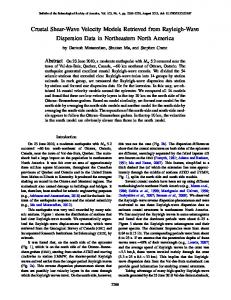
minimum of the sum of the square of errors. In harmony with [8], our database shows that the geologic age has a significant effect on shear wave velocity. The difference in behavior is outlined from Fig. 13, which shows the shear wave velocities vs CPT cone tip resistance separated by geologic groups created in chapter II. The highest variability belongs to the group b) (squares), which was seen in chapter IV also. Each group of points from the other three geologic conditions also plot along a line with lower deviation. The optimization analysis was made for each group and for some combined groups. As presented in chapter IV, very good agreement was found for group a) for all methods, and the best

(14)

 D 0 .249

400

0

(13a)

c

0 .321

500

Gr-a

To improve the existing equations for estimating vs for Hungarian geological conditions, we set out from (4) and (8). For (8) we checked the effect of changing the power function as well. Therefore the following base equations were used: b

 Ic

0

V. NEW RECOMMENDATION

v s  a  q t  Ic  D d

0 .201

600

shear wave velocity, vs [m/s]

C. Conclusion Based on the comparison results of existing formulae to estimate shear wave velocity from CPT data, the following conclusions can be drawn:  generally the best estimation can be reached with (8) recommended by [10], meanwhile (4) can gives also relative good estimations. These two are recommended to apply to Hungarian soils.  Shear wave velocity calculated by (1) has more than 17% relative error compared to measured values, and the deviation of the estimation is also high, therefore it is not recommended to be applied.  The existing recommendations give relatively good estimation for shear wave velocity of fluvial deposits, both for river sediment and sea sediment. With increasing the geologic age, the deviation of the estimation also increases.  For the aeolian deposits the existing recommendations need to be improved, because most of them underestimate the shear wave velocity with high error.

one was given by [10]. When optimized this recommended correlation is not improved significantly, the coefficient of determination becomes also R2 = 0.88 for (13b) and (13c) with the slope of the trend line equal 1. The best fit can be reached based on (13a), where the R2 = 0.91 with



Although only a few data are available for Tertiary age soils, the results show tendencies similar to group b) for (A) and (R) recommendations. These two have an average error of about zero with less than 15% deviation. On the other hand, (1) gives an average 15% overestimation, and shear wave velocity calculated by (9) deviates more than 8% from the measured data.

Gr-a vsm = 1.0∙vse R2 = 0.91

400

Gr-b vsm = 1.0∙vse R2 = 0.39

300

200

100 Na-Gr-a Na-Gr-b 0 0

100

200 300 400 500 estimated shear wave velocity, vse [m/s]

Fig. 14 Estimated vs measured vs for group a (14) and b (15)

Fig. 14 represents the estimated vs compared to measured values for group a) and b), where the grey circles belong to group a, and the squares to group b). The continuous line is vsm = vse. For group a), 90% of the data are bounded by an area bordered with vsm = (1±0.14)∙vse lines. The estimated shear wave velocity for all new equations show very strong correlation to measured data. For group b), the three new equations give similar results. All of them have almost the same coefficient of determination (0.37-0.39), which show lower correlations. The best fit can

345



v s  13 . 25  q t

0 .412

 Ic

0 .819

(15)

v s  4 .0  q t

0 .388

 Ic

0 .802





(16b)





(16c)

v s  10 0.522 Ic  2 .341  q t   v 0  / p a



v s  10 0.672 Ic  2.393  q t   v 0  / pa

0 .5

0 .446



v s  10

 q t   v 0  / p a



0 .5

0 .423

(19)

Na vsm = 1.0∙vse R2 = 0.44

400

300

200

The worst estimations can be found in the literature for Aeolian sediments, which underestimate the shear wave velocity by more than 20% with relatively high deviation. By improving (8), the average error can be reduced to almost zero, but the deviation is still relative high. In Fig 15, the white diamonds represents this, and is estimated by 0 .497 I c  2 .075



500

(16a)

 D 0 .017

v s  10 0.538 Ic 1 .713  q t   v 0  / p a

100

0 0

100

(17)


Fig. 16 Estimated vs measured vs for Quaternary age soils

500



This means the best fit is independent of depth (overburden stress). It should be noted that the low power function of depth always means overburden stress has less effect on shear wave velocity. Combining the fluvial deposits together (Gr-a + Gr-b) gives a coefficient of determination equal to R2 = 0.52 that can be reached by all of the following equations:

The best estimation for the Quaternary age soils (group a) + group b) + group c)) comes from (13b) (see Fig. 16.), but the other two have similar results based on the coefficients of determination. In Fig. 16, the 80% boundary of the points are drawn with dashed lines, which deviates by 25% from the vsm = vsm line. The recommended equation is


achieved by an equation based on (13a) with the following form:

Na vsm = 1.0∙vse R2 = 0.57

400

Nb vsm = 1.0∙vse R2 = 0.37

300

200

100 Na-Gr-c Nb-Gr-c

0 0

100


Fig. 15 Estimated vs measured vs for group c

A fairly strong correlation can be achieved by optimizing (13a), where in addition to the slope of the trend line being equal to 1, the coefficient of determination has increased (black diamonds on Fig. 15, R2 = 0.57). The resulting equation is v s  25 . 69  q t

0 .176

 Ic

0 .713

 D 0 .13

(18)


For Pleistocene age soils improved correlation is not found based our analysis, the coefficient of determination is only R2 = 0.34-0.38, perhaps because of the different origins (fluvial, Aeolian). The group d) can be divided into two subgroups because the data comes from two different sites. A majority of the shear wave velocities were measured in Budapest, where the Miocene age layers are situated at depth 13-20 m. Here the vs is changing between about 300-350 m/s. Only six data points come from Paks-1, where the Pannonian base layer is at a depth of 28-34 m with higher shear wave velocities (380-480 m/s). For the whole group d) and separately for the Miocene age soils, effective improvement is not reached with optimization of equations based on CPT data. The Pannonian base layer was not analyzed separately because of the small number of data. A fairly strong correlation is achieved when calculating shear wave velocity by v s  91 . 03  D 0 .456

(20)

which is a similar form to what the literature suggests for estimating shear wave velocity [14]. Fig. 17 shows the two subgroups of group d). The minimum of the sum of the errors squared for all data can be reached also based on (13a). The equation

346



v s  11 . 97  q t

0 .262

 Ic

0 .709

(21)

 D 0 .107

gives R2 = 0.43, which means perceptible, but not very useful, correlations. 600

Na vsm = 1.0∙vse R2 = 0.63



500

based on least squares regression. Based on this study the following preliminary recommendations can be given according to the geologic conditions:  for Holocene fluvial deposits (eg.next to the Tisza River), (14) is recommended,  if there is any information about the origin: for fluvial deposit (16a) and for Aeolian sediment (18),  if there is no information about the origin, but it is surely a quaternary age soil, use (19)  for more general cases use (21).

400

REFERENCES [1]

300 200

[2]

100

Gr-d-mi

[3]

Gr-d-pa

0 0

100

200

300

400

500

estimated shear wave velocity, vse [m/s]

Fig. 17 Estimated vs measured vs for group d

[4] [5]

VI. CONCLUSIONS Dynamic soil properties are important in foundation vibration problems, earthquake site response analysis, site classification according to EC8-1, etc. There are several techniques to measured dynamic properties in the field or laboratory, but in many cases budgets of the geotechnical investigations does not allow these. On the other hand, the CPT is frequently used for geotechnical design. Considering this, the aim of this paper is to analyze and improve the existing recommendations for estimating shear wave velocity from CPT data for Hungarian soil conditions. Altogether more than 280 data from 7 locations in Hungary were used in our research. These data can be divided into four groups according to geological conditions: (a) Holocene age fluvial deposits, (b) Pleistocene age fluvial deposits, (c) Pleistocene age Aeolian deposits and (d) tertiary age deposits. Four existing recommendations were compared: (1) given in [6], (4) given in [8], (8) given in [10] and (9) given in [11]. Based on a comprehensive comparison study, the following can be pointed out:  the recommendations underestimate the shear wave velocity in general,  for group a), b), and d), the average error is almost zero, but for group c) the difference is more than 20%,  the best fit was found for group a by (8) with R2 = 0.88,  for the other 3 groups the deviation of error is relatively high; about 15-20%,  generally the (8) gives the best results, but still with high deviation. According to the results of the comparison analysis, the constants for (4) and (8) were optimized with Excel Solver


[6]

[7]

[8]

[9]

[10] [11] [12] [13] [14] [15]

347

J. Schneider, A. McGillivray and P. Mayne, “Evaulation of SCPTU intra-correlations at sand sites in the Lower Mississippi River valley, USA” in Proceedings, 2th International Conference on Geophysical and Geotechnical Site Characterization (ISC’2), Rotterdamm, Millpress, pp. 1003-1010, 2004 R.F. Obrzud, “On the use of the Hardening Soil Small Strain model in geotechnical practice, in Numerics in Geotechnics and Structures, Elmepress International, Lausanne, pp. 15-32, 2010 G. Baldi, R. Bellotti, V. Ghionna, M. Jamiolkowski and L. Presti, “Modulus of sands from CPTs and DMTs” in Proceedings 12th International Conference on Soil Mechanics and Foundation Engineering, Vol. 1 pp. 165-170, Rio de Janeiro, Balkema, Rotterdam, 1989. P. Robertson, C. Woeller, and W. Finn, “Seismic cone penetration test for evaluating liquefaction potential”. Canadian Geotechnical Journal, Vol 29, pp. 686-695, 1992 P.W. Mayne and J.G. Rix, “Correlations between shear wave velocity and cone tip resistance in natural clays,” Soils and Foundations, JSSMFE, Vol 35(2), pp 107-110, 1995. Y. Hegazy and P. Mayne, “Statistical correlations between vs and cone penetration data for different soil types” Proceedings, International Symposium on Cone Penetration Testing, CPT ’95, Linkoping, Sweden, Swedish Geotechnical Society, pp. 173-178, 1995 C. Madiai and G. Simoni, “Shear wave velocity-penetration resistance correlation for Holocene and Pleistocene soils of an area in central Italy” Proceedings, 2th International Conference on Geophysical and Geotechnical Site Characterization (ISC’2), Rotterdamm, Millpress, pp. 1687-1694, 2004. R.D. Andrus, N.P. Mohanan, P. Piratheepan B.S. Ellis and T. L. Holzer, “Predicting shear wave velocity from cone penetration resitance”, in Proceedings, 4th International Conference on Earthquake Geotechnical Engineering, Thessaloniki, Greece, Paper No. 1545, 2007 L. Karl, W. Haegeman and G. Degrade, “Determination of the material damping ratio and the shear wave velocity with the Seismic Cone Penetration Test, Soil Dynamics and Earthquake Engineering, Vol 26. pp 1111-1126, 2006 P.K. Robertson, “Interpretation of cone penetration tests - a unified approach. Canadian Geotechnical Journal, Vol 46. pp. 1337-1355. 2009 L. Tonni and P. Simonini, “Shear wave velocity as function of cone penetration test measurements in sand and silt mixture”. Engineering Geology, Vol 163, pp. 55-67 2013. P.K. Robertson and C.E. Wride, “Evaulating cyclic liquefaction potential using the cone penetration test, Canadian Geotechnical Journal, Vol. 35. pp 442-459, 198 P.K. Robertson, R.G. Campanella, D. Gillespie and A. Rice, “Seismic CPT to measure in situ shear wave velocity, in ASCE J. GED, Vol 112 (8), pp 791-803, 1986 S.L. Kramer: Geotechnical Earthquake Engineering, Prentice Hall, Upper Saddle River, New Jersey, 1996. JJ.M. Brouwer: In-situ soil testing, 2007, online book: http://www.conepenetration.com/online-book/
