SHERLOCK: MODELING STRUCTURED KNOWLEDGE IN IMAGES

Under review as a conference paper at ICLR 2016

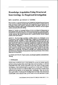
S HERLOCK : M ODELING S TRUCTURED K NOWLEDGE IN I MAGES Mohamed Elhoseiny1,2 , Scott Cohen1 , Walter Chang1 , Brian Price1 , Ahmed Elgammal2 1 2 Adobe Research Department of Computer Science, Rutgers University

arXiv:1511.04891v3 [cs.CV] 8 Jan 2016

A BSTRACT

1

How can we build a machine learning method that can continuously gain structured visual knowledge by learning structured facts? We address this question by proposing a problem setting where training data comes as structured facts in images, including (1) objects (e.g., ), (2) attributes (e.g., ), (3) actions (e.g., ), and (4) interactions (e.g., ). Each structured fact has a semantic language view (e.g., < boy, playing>) and a visual view (an image with this fact). A human is able to efficiently gain visual knowledge by learning facts in a never ending process, and we believe in a structured way (e.g., understanding “playing” is the action part of , and hence can generalize to recognize if is also understood). Inspired by human visual perception, we propose a model that (1) is able to learn a representation which covers different types of structured facts, (2) could flexibly get fed with structured fact language-visual view pairs in a never ending way to gain more structured knowledge, (3) could generalize to unseen facts, and (4) allows retrieval of both the fact language view given the visual view and vice versa. We also propose a novel method to generate hundreds of thousands of structured fact pairs from image caption data to train our model, and which can be useful for other applications. I NTRODUCTION

The vast majority of the existing visual recognition methods assume a fixed dictionary of visual facts. However, visual knowledge that we gain in our world is highly dynamic. Furthermore, different types of facts are modeled as different systems (e.g., different systems for object recognition, action recognition, interaction recognition, scene recognition, attribute recognition, etc). A human visual system is able to efficiently gain visual knowledge by learning facts of different types in a never ending process and from a few examples. Inspired by human visual perception, we present the problem of universal visual recognition, where we propose one Language&Vision approach that is able to learn objects, scenes, their attributes, their actions, and their interactions with other objects or scenes. Our fundamental idea for learning these facts together starts with introducing structure in their labels, categorizing labels into first order, second order and third order facts; see Fig. 1. First Order Facts are object categories and scenes (e.g., , , ). Second Order Facts are objects performing actions or attributed objects (e.g., , Figure 1: Sherlock Problem: Gaining Structured ). Third Order Facts Visual Knowledge are interactions and positional information are represented by (e.g. , ). Although it is common to label visual facts as only first order (e.g., , ), we argue that information in an image is usually more specific but we just label them in a limited way restricted to the task in hand. For example, we may find a , , or not just a person or a car. This motivates the structure we introduce to the label, where the S is the main subject of the fact and P is the attribute or action that modifies the appearance of S. In case of interaction, O represent the interacting object and P defines the interaction itself. Inspired from the concept of language modifiers, we then propose to model and facts as visual modifiers to . For example, the second order fact is a visual modifier for , and the third order fact is a visual modifier for both the second order fact and the first order fact . We argue that what makes recognition sometimes hard for some objects is the space of visual modifiers and how common it is, i.e., it might be easier to recognize a “person” modified by “standing” modifier (standing visual modifier) compared to a person doing acrobatics . We think that the reason is that some visual modifiers are common (e.g., standing) and others are rare (e.g., doing acrobatics) during training, another view of the long-tail problem. An important observation is that the visual modifiers are more related to detailed appearance of an object like pose and color, which could be untangled in a visual recognition deep network and introduces a need to be modeled by separate filters that we propose in this work; detailed in Model 2 in Sec. 4 . Hence, we propose to model universal visual recognition along three continuous hyper-dimensions φS , φP , and φO , where φS ∈ RdS : covers the space of object categories or scenes S. φP ∈ RdP : covers the space of actions, interactions, attributes, and positional information. φO ∈ RdO : covers the space of interacting objects, scenes that interact with S. For instance, first order facts like , , live in a hyper-plane in the φP × φO space; see Fig. 2. Second order facts (e.g., , ) live as a hyper-line that is parallel to φO axis. Finally, a third order fact like is a point in the φS × φP × φO visual perception space. Meanwhile, this point lies on the hyper-plane and the hyperline. While we focus our experiments on , , , our proposed setting assumes that there should be at least one non-wild card * in a training example including for example ; see Fig 2. We argue that modeling visual recognition based on this notion gives it a generalization capability since it allows us to learn facts like , , during training, and it will be an expected behavior to be able to recognize during testing even is never seen before. Another example is if a model learned the facts , , and , it should be able to recognize an unseen fact . We observe this in our results in several unseen cases. We model structured knowledge in images as a problem that comes with two views, one in the visual domain V and one in the language domain L. Let f be a structured fact, fv ∈ V denoting the view of f in the visual domain and fl ∈ L denoting the view of f in the language domain. For instance, an annotated fact with language view fl = would have a corresponding visual view fv as an image where this fact occurs; see Fig. 3. Our goal is to learn a representation that covers first-order facts (objects), secondorder facts (actions and attributes), and third-order facts (interaction and positional facts). We represent all types of facts as an embedding problem into what we call “structured fact space”. We define “structured fact space” as a learning representation of the φS ∈ RdS , φP ∈ RdP , and φO ∈ RdO hyper-dimensions (Fig. 3). We denote the embedding functions from a visual view of a fact V fv to φS , φP , and φO as φV S (fv ), φP (fv ), and φV (f ), respectively. Similarly, we denote the O v embedding functions from a language view of a L fact fl to φS , φP , and φO as φL S (fl ), φP (fl ), and L φO (fl ), respectively. We denote the concatenaFigure 3: Problem Definition 2


tion of the visual view hyper-dimensions’ embedding as φV (fv ), and the language view hyperdimensions’ embedding as φL (fl ), where φV (fv ) and φL (fl ) are visual embedding and language embedding of f , respectively: V V L L L L (1) φV (fv ) = [φV S (fv ), φP (fv ), φO (fv )], φ (fl ) = [φS (fl ), φP (fl ), φO (fl )] Modeling the connection between the provided structured facts in its language form and its visual view facilitates gaining richer visual knowledge, which is our focus in this paper. We further show that modeling universal visual perception as a Language&Vision problem have several advantages: (1) highly dynamic: can be given fact language-visual view pairs in a never ending way to gain more structured knowledge. (2) generalization: could generalize to unseen facts. (3) bi-directional: allows retrieval of both the fact language view given the visual view and vice versa. (4) wild-cards: In order to model different types of facts in one model, we present the notion of visual modifiers, where higher order facts (e.g., ) are modeled as visual modifiers of lower order facts. We train using a novel wild-card loss function which allows learning all different types of facts in one model, detailed in Sec. 4. Since the proposed setting is aiming for a model that has an eye for details and potentially allows higher order reasoning (Fig. 1), we denote this problem as the Sherlock Problem. Data Collection in our setting: This is a new setting and in order to train a model for our setting, we needed to collect structured fact annotations in the form of (language view, visual view) pairs (e.g., as the language view and an image with this fact as a visual view). This is a challenging task. We started by manually annotating and mining several existing datasets to extract structured fact annotations, which we found limiting for both the dataset size and for covering different types of facts (Sec. 3). One of the most interesting relevant works is the Never Ending Image Learner (NEIL) (Chen et al., 2013), where they showed that visual concepts predefined in an ontology can be learnt by collecting its training data from the web. In a follow-up work, Divvala et al. (2014) collected images from the web for concepts related to a predefined object using GoogleN-gram data. This opens the question of whether we can collect structured fact annotations from the web. There are two issues we face in our setting. First, it is difficult to define the space of structured visual knowledge and then search for it. Second, using Google image search is not reliable to collect data for concepts with fewer images on the web. The main assumption for this method depends on both the likelihood that the top retrieved image belongs to the searched concept, and the availability of images annotated with the searched concept. These problems motivated us to propose a novel method to automatically annotate structured facts by processing image caption data since structured facts in image captions are highly likely to be located in the image. Our Sherlock Automatic Fact Annotation (SAFA) method extracts fact language views from image captions and then localizes the facts to image regions to get visual views. SAFA collected tens of thousands of unique knowledge annotations within hundreds of thousands of images in just several hours. Contributions. There are three main contributions in this paper: (1) We introduce the Sherlock problem of modeling universal visual recognition and propose the visual modifiers notion that enables learning structured facts of different types and performs both-view retrieval (retrieve structured fact language view (e.g. ) given the visual view (i.e. image) and vice versa). (2) We propose an automatic stuctured fact annotation method based on sophisticated Natural Language Processing methods for acquiring high quality structured fact annotation pairs at large scale from free-form image descriptions. We applied the pipeline to MS COCO Lin et al. (2014) and Flickr30K Entities Plummer et al. (2015); Young et al. (2014) image caption datasets. In total, we build a structured fact dataset of more than 816, 000 language&image-view fact pairs covering more than 202, 000 unique facts in the language view. (3) We develop a novel learning representation network architecture to jointly model the structured fact language and visual views by mapping both views into a common space and using a wild card loss to uniformly represent first, second, and third order facts. Our modeling approach is scalable to new facts without any change to the network architecture.

2

R ELATED W ORK

In order to make the contrast against related work clear, we start by stating the scale of facts we are modeling in this work. Let’s assume that |S|, |P|, and |O| denotes the number of unique subjects, unique predicates, and unique objects, respectively. The scale of unique second and third order facts is bounded by |S| × |P| and |S| × |P| × |O| possibilities respectively, which can easily reach millions 3


of unique facts and needs careful attention while designing a model maintaining the structure we aim at. The data we collected in this work has thus far reached 202,000 unique facts (814,000 images). (A) Modeling Visual facts in Discrete Space: Visual Recognition tasks like object or activity recognition have been typically addressed as a mapping function g : V → Y, where Y is discrete set of classes 1 → K. The function g was traditionally learned over engineered features like variants of SIFT features (e.g., Bosch et al. (2007)), and have recently been learned using deep learning (e.g., Simonyan & Zisserman (2015); Szegedy et al. (2015). Nowadays, different methods/systems are built to recognize facts in images by modeling a different g : V → Y , where Y is constrained to certain facts for each approach. Examples of different Y for different facts include (1) object categories, (e.g., Simonyan & Zisserman (2015)), (2) attributes (e.g. Zhang et al. (2014)), (2) attributed objects < car, red > Chen & Grauman (2014), (3) scenes (e.g., Zhou et al. (2014)), (4) activities (e.g., Gkioxari & Malik (2015), and (5) interactions Antol et al. (2014a). This opens the question of why we build different systems or approaches for these related tasks since images usually contain objects with particular attributes performing an action or interacting with another object. We think that there are several limitations in modeling visual recognition as g : V → Y. (1) Grouping visual facts and modeling each group by a different g, while a human visual perception system is able to incrementally learn visual facts (objects, interactions, actions, attributes classes, etc) as one system. In the real world, this means that we need to group each visual fact type in order to deal with a different recognition system for each group and then retrain several models. (2) Adding a new fact leads to changing the architecture, meaning adding thousands of parameters and re-training the model (e.g., needed for adding a new output node). If we used VGGNet for instance on the scale of 202K facts, the number of parameters in the softmax layer alone gets very close to 1 billion parameters. GPU memory does not fit this number of parameters and makes learning a big challenge. (3) While the majority of the existing benchmarks have at least tens of examples per fact (e.g., imageNet (Deng et al., 2009)), a more realistic assumption for visual recognition is that there might not be enough examples for the newly added examples to learn the new class, which introduces a learning problem. This problem is know as the long-tail, where several works have been proposed to deal with in the object recognition setting following a ditribution similar to Zipf’s law (Zipf, 1935; Salakhutdinov et al., 2011).(4) These models are only uni-directional from V to Y. (B) Modeling zero/few shot fact learning by attributes: One of the most successful ideas for learning from few examples per class is by using semantic output codes or attributes as an intermediate layer between features and class. Formally, g is composition of two function g = h(a(·)), where a : V → A, and h : A → Y (Palatucci et al., 2009). The main idea is to collect data that is sufficient to learn about the intermediate attribute layer, where classes are then represented by these attributes to faciltate zero-shot/few-shot learning. However, Chen & Grauman (2014) realize that attribute appearance is dependent on the class, as opposed to these earlier models (Palatucci et al., 2009; Lampert et al., 2009). Although Chen & Grauman (2014)’s assumption is more realistic, learning different classifiers for each category-attribute pair introduces the scalability and learning difficulties pointed out in (A), limits the model’s applicability, and still restricts the model to certain groups of facts. In contrast, our goal is a method that can learn any visual fact in an incremental way. It is worth mentioning that there is a huge body of work in incremental learning (e.g. Bendale & Boult (2015)), but it mainly focuses on the object recognition task and assumes labels Y lives in a discrete space (not tractable for universal visual recognition). Furthermore Bendale & Boult (2015) also assumes that each image has only one fact, which is not a restriction in our work (e.g., same image could have and ). Also, the notion of similar classes is not addressed in the vast majority of these works. For instance, is expected to be more similar to than to , which makes a stronger motivation for learning facts in a continuous space. (C) Object Recognition in continuous space using Vision and Language: Recent works in language and vision involve using unannotated text to improve object recognition and to achieve zero-shot learning. The following group of approaches model object recognition as a function g(v) = arg maxy s(v ∈ V, y ∈ Y), where s(·, ·) is a similarity function between image v and class y represented by text. In (Frome et al., 2013), (Norouzi et al., 2014) and Socher et al. (2013), word embedding language models (e.g., Mikolov et al. (2013)) were adopted to represent class names as vectors. Their framework maps images into the learned language model and then does classification in that space. In addition to that our setting is different, imageNet dataset in their case has 1000 object facts with thousands of examples per class. Our setting has two orders of magnitude

4


Figure 4: Sherlock Automatic Fact Annotation (SAFA) more facts with long-tail distribution. Conversely, other works model the mapping of unstructured text descriptions for classes into a visual classifier (Elhoseiny et al., 2013; Ba et al., 2015). We are extending the visual recognition task to the scale of millions of facts, not only object recognition but also understanding their attributes, actions, and interactions in one model. Our labels are also structured, where we handle missing parts like P and O in examples and O in , which enables our method to learn facts of different types by the wild-card loss we introduce. Furthermore, we propose the visual modifiers notion, which motivates us to learn separate branches of convolutional filters that outperforms more straightforward convolutional baselines that we designed for this task; see Sec 4.

3

DATA C OLLECTION OF S TRUCTURED FACTS

In order to train a model that connects the structured fact language view in L with its visual view in V, we need to collect large scale data in the form of (fv , fl ) pairs. Data collection especially for large scale problems is a challenging task. It is further challenging in our setting since our knowledge model relies on the localized association of a structured language fact fl with an image fv when such facts occur. In particular, it is a complex task to collect annotations especially for second-order facts and third-order facts . Also, multiple structured language facts could be assigned to the same image (e.g., and ). If these facts refer to the same man, the same image example could be used to learn about both facts. Table 1: Our fact augmentation of six existing datasets Unique language views f Number of ( f , f ) pairs We began our data collection by aug< S > . < S, P > . < S, P, O > . total < S > < S, P > < S, P, O > total images INTERACT 0 0 60 60 0 0 3171 3171 menting existing datasets with fact VisualPhrases 11 4 17 32 3594 372 1745 5711 Stanford40 0 11 29 40 0 2886 6646 9532 language view labels fl : PPMI (Yao PPMI 0 0 24 24 0 0 4209 4209 SPORT 14 0 6 20 398 0 300 698 & Fei-Fei, 2010), Stanford40 (Yao Pascal Actions 0 5 5 10 0 2640 2663 5303 Union 25 20 141 186 3992 5898 18734 28624 et al., 2011), Pascal Actions (Everingham et al.), Sports (Gupta, 2009), Visual Phrases (Sadeghi & Farhadi, 2011), INTERACT (Antol et al., 2014b) datasets. The union of these 6 datasets resulted in 186 facts with 28,624 images as broken out in Table 1. l

v

l

We also extracted structured facts from the Scene Graph dataset (Johnson et al., 2015) with 5000 manually annotated images in a graph structure from which first-, second-, and third-order relationships can be easily extracted. We extracted 110,000 second-order facts and 112,000 third-order facts. The majority of these are positional relationships. We further propose a method to automatically collect structured fact annotations from datasets that come in the form of image-caption pairs, which can more quickly provide useful facts (Sec. 3.1). Our proposed method opens the door for easy continual fact collection in the future from caption datasets and even the web or in general any naturally occurring documents with image descriptions. 3.1 S HERLOCK AUTOMATIC FACT A NNOTATION (SAFA) FROM IMAGES WITH CAPTIONS We automatically obtain a large quantity of high quality facts from caption datasets using natural language processing methods. Caption writing is free-form and an easier task for crowd-sourcing workers than labeling second- and third-order tasks, and such free-form descriptions are readily available in existing image caption datasets (e.g. MS COCO Lin et al. (2014)). In our work, we focused on the MS COCO image caption dataset (Lin et al., 2014) and the newly collected Flickr30K entities (Plummer et al., 2015) to automatically collect new structured fact annotations. In contrast to the Scene Graph dataset of 5000 manually annotated scenes, we automatically extracted facts from more than 600,000 captions associated with more than 120,000 MS COCO scenes, and facts from more than 150,000 captions associated with more than 30,000 scenes for the Flickr30K dataset; this provided us with 30 times more additional coverage over the initial structured facts from the Scene Graph dataset. 5


We propose SAFA as a two step automatic annotation process: (i) fact extraction from captions, and (ii) fact localization in images. First, the captions associated with the given image are analyzed to extract sets of clauses that are considered as candidate , and facts. We extract clauses using two state-of-the-art methods: Clausie Del Corro & Gemulla (2013) and Sedona-3.0 (see Appendix B for details). Clauses form facts but are not necessarily facts in our context by themselves until they have a corresponding visual view. Captions can provide a tremendous amount of information to image understanding systems. However, developing NLP systems to accurately and completely extract structured knowledge from free-form text is an open research problem. We addressed several challenging linguistic issues by evolving our NLP pipeline to: 1) correct many common spelling and punctuation mistakes, 2) resolve word sense ambiguity within clauses, and 3) learn a common spatial preposition lexicon (e.g., ”next to”, ”on top of”, ”in front of”) that consists of over 110 such terms, as well as a lexicon of over two dozen collection phrase adjectives (e.g., ”group of”, ”bunch of”, ”crowd of”, ”herd of”). These strategies allowed us to extract more interesting structured knowledge for learning. Second, we try to localize these clauses within the image (see Fig. 4). The subset of clauses that are successfully located in the image are saved as fact annotations for training our model. We collected 146,515, 157,122, and 76,772 annotations from Flickr30K Entities, MS COCO training, and validation sets, respectively. Even though we excluded some types of clauses that were likely to produce incorrect annotations, we achieved a total of 380,409 second- and third-order fact annotations. We present statistics of the automatically collected facts in Appendix. C. We note that the process of localizing facts in an image is constrained by information in the dataset. For MS COCO, the dataset contains object annotations for about 80 different objects as provided by the training and validation sets. This allowed us to localize first-order facts for objects using bounding box information. In order to locate higher-order facts in images, we started by defining visual entities. For the MS COCO dataset (Lin et al., 2014), we define a visual entity as any noun that is either (1) one of the MS COCO dataset objects, (2) a noun in the WordNet ontology (Miller, 1995; Leacock & Chodorow, 1998) that is an immediate or indirect hyponym of one of the MS COCO objects (since WordNet is searchable by a sense and not a word, we performed word sense disambiguation on the sentences using a state-of-the-art method (Zhong & Ng, 2010)), or (3) one of the SUN dataset scenes (Xiao et al., 2010). We expect visual entities to appear either in the S or the O part (if it exists) of a candidate fact fl . This allows us to then localize facts for images in the MS COCO dataset. Given a candidate third-order fact, we first try to assign each S and O to one of the visual entities. If S and O elements are not visual entities, then the clause is ignored. Otherwise, the clauses are processed by several heuristics, detailed in Appendix A. For instance, our method takes into account that grounding the plural ”men” in the fact may require the union of multiple ”man” bounding boxes. In the Flickr30K Entities dataset (Plummer et al., 2015), the bounding box annotations are presented as phrase labels for sentences (for each phrase in a caption that refers to an entity in the scene). A visual entity is considered to be a phrase with a bounding box annotation or one of the SUN scenes. Several heuristics were developed and applied to collect these fact annotations, e.g. grounding a fact about a scene to the entire image; see details in Appendix A.

4

S HERLOCK M ODELS

In this section, we first illustrate our learning representation and how it is applied to different fact types. Then, we present the proposed models. 4.1

V ISUAL M ODIFIERS AND WILD - CARD REPRESENTATION

Third-order facts can be directly embedded in the structured fact space using Eq. 1 with φV (fv ) for the image view and φL (fl ) for the language view. Based on our “fact modifier” observation, we propose to represent both first- and second-order facts as wild cards “∗”, as illustrated in Eq. 2 and 3. First-Order Facts wild-card representation V V L L L L φV (fv ) = [φV S (fv ), φP (fv ) = ∗, φO (fv ) = ∗], φ (fl ) = [φS (fl ), φP (fl ) = ∗, φO (fl ) = ∗] Second-Order Facts wild-card representation V V L L L L φV (fv ) = [φV S (fv ), φP (fv ), φO (fv ) = ∗], φ (fl ) = [φS (fl ), φP (fl ), φO (fl ) = ∗] 6

(2) (3)


Figure 5: Sherlock Models. See Fig. 3 for the full system. Setting φP and φO to ∗ for first-order facts is interpreted to mean that the P and O modifiers are not of interest for first-order facts, which is intuitive. Similarly, setting φO to ∗ for second-order facts indicates that the O modifier is not of interest for single-frame actions and attributes. If an image contains lower order fact such as , then higher order facts such as or may also be present. Hence, the wild cards (i.e. ∗) of the lower order facts are not penalized during training in our loss described later in this section; see Fig. 2 for illustration and examples of first order facts as hyper-planes and second-order facts as hyper-lines. 4.2

P ROPOSED M ODELS

We propose a two-view structured fact embedding model with four properties: (1) it can be continuously fed with new facts without changing the architecture, (2) it is able to learn with wild cards to support all types of facts, (3) it can generalize to unseen facts, (4) it allows two way retrieval (i.e., retrieve relevant facts in language view given an image, and retrieve relevant images given a fact in a language view). Satisfying these properties can be achieved by using a generative model p(fv , fl ) that connects the visual and the language views of f , where more importantly fv and fl inhabit a continuous space. Our method is to model p(fv , fl ) ∝ s(φV (fv ), φL (fl )), where s(·, ·) is a similarity function defined over the structured fact space denoted by S. Our objective is that two views of the same fact should be embedded so that they are close to each other. The question now is how to model and train φV (fv ), and φL (fl ). We model φV (fv ) as a CNN encoder (e.g., Krizhevsky et al. (2012); Simonyan & Zisserman (2015)), and φL (fl ) as RNN encoder (e.g., Mikolov et al. (2013); Pennington et al. (2014)) due to their recent success as encoders for images and words, respectively. We propose two models for learning facts, denoted by Model 1 and Model 2. Model 1 and 2 share the same structured fact language embedding/encoder but differ in the structured fact image encoder. We start by defining an activation operator ψ(θ, a), where a is an input, and θ is a series of one or more neural network layers (may include different layer types, e.g., convolution, one pooling, then another convolution and pooling). The operator ψ(θ, a) applies θ parameters layer by layer to finally compute the activation of the θ subnetwork given a. Model 1 (structured fact CNN image encoder): In Model 1, a structured fact is visually encoded by sharing convolutional layer parameters (denoted by θcv ), and fully connected layer parameters (denoted by θvu ); see Fig. 5(a). Then WSv , WPv , and WOv transformation matrices are applied to V V produce φV S (fv ),φP (fv ) , and φO (fv ): u c S V P V O b = ψ(θv , ψ(θv , fv )), φV (4) S (fv ) = Wv b, φP (fv ) = Wv b, φO (fv ) = Wv b. Model 2 (structured fact CNN image encoder): In contrast to Model 1, we use different convolutional layers for S that for P and O, inspired by the idea that P and O are modifiers to S (Fig. 5(b)). Starting from fv , there is a common set of convolutional layers, denoted by θvc0 , then the network splits into two branches, producing two sets of convolutional layers θvcS and θvcP O , followed by two sets of fully connected layers θvuS and θvuP O . If we define the output of the common S,P,O layers as d = ψ(θcv0 , fv ) and the output of the P,O column as e = ψ(θvuP O , ψ(θvcP O , d)), then S uS cS V P V O φV (5) S (fv ) = Wv ψ(θv , ψ(θv , d)), φP (fv ) = Wv e, φO (fv ) = Wv e. Structured fact RNN language encoder: The structured fact language view is encoded using RNN S L P word embedding vectors for S, P and, O. Hence φL S (fl ) = RNNθl (fl ), φP (fl ) = RNNθl (fl ), L O S P O φO (fl ) = RNNθl (fl ), where fl , fl , and fl are the Subject, Predicate, and Object parts of fl ∈ L. For each of them, the literals are dropped. If any of flS , flP , or flO contain multiple words, we compute the average vector as the representation of that part. We denote the RNN language encoder parameters by θL . In our experiments, θl is fixed to a pre-trained word vector embedding model (e.g. Mikolov et al. (2013); Pennington et al. (2014)) for flS , flP , and flO ; see Fig 5(c). 7


Loss function: One way to model p(fv , fl ) for Model 1 and Model 2 is to assume that p(fv , fl ) ∝= exp(−lossw (fv , fl )) and minimize the distance lossw (fv , fl ) defined as L 2 f V L 2 f V L 2 lossw (fv , fl ) = wSf · kφV S (fv ) − φS (fl )k + wP · kφP (fv ) − φP (fl )k + wO · kφO (fv ) − φO (fl )k . Thus we minimize the distance between the embeddings of the visual view and the language view. Our solution to penalize wild-card facts is to ignore the wild-card modifiers in the loss. Here wSf = 1, f f wPf = 1, wO = 1 for facts , wSf = 1, wPf = 1, wO = 0 for facts, and wSf = 1, f f wP = 0, wO = 0 for facts. Hence lossw does not penalize the O modifier for second-order facts or the P and O modifiers for first-order facts, which follows our definition a wild-card modifier. Testing (Two-view retrieval): After a Sherlock Model is trained (either Model 1 or 2), we embed all the test fv by φV (fv ), and all the test fl with φL (fl ). For language view retrieval given an image, we compute the cosine similarity between a given φV (fv ) in the test set and all the φL (fl ), which indicates relevance for each fl for the given fv . For image retrieval given an fl , we compute the cosine similarity between φL (fl ) and all φV (fv ) in the test set, which indicates relevance for each fv for the given fl . For first and second order facts, the wild-card part is ignored in the similarity.

5

E XPERIMENTS

5.1 SAFA EVALUATION We start with our evaluation of the automatically collected annotations by the two-step SAFA process, where fact language views are first extracted from the caption, then the facts are located in the image. We propose three questions to evaluate each annotation: (Q1) Is the extracted fact correct (Yes/No)? The purpose of this question is to evaluate errors captured by the first step, which extracts facts by Sedona or Clausie. (Q2) Is the fact located in the image (Yes/No)? In some cases, there might be a fact mentioned in the caption that does not exist in the image and is mistakenly considered as an annotation. (Q3) How accurate is the box assigned to a given fact (a to g)? a (about right), b (a bit big), c (a bit small), d (too small), e (too big), f (totally wrong box), g (fact does not exist or other). Our instructions on these questions to the participants can be found in this url Eval (2015). We evaluate these three questions for the facts that were successfully assigned a box in the image, because the main purpose of this evaluation is to measure the usability of the collected annotations as training data for our model. We created an Amazon Mechanical Turk form to ask these three questions. So far, we collected a total of 10,786 evaluation responses, which are an evaluation of 3,595 (fv , fl ) pairs (3 responses/ pair). Table 2 shows the evaluation results, which indicate that the data is useful for trainTable 2: SAFA Evaluation by MTurk workers % Dataset (responses) Q1 Q2 Q3 ing, since≈83.1% of them yes no Yes No a b c d e f g are correct facts with boxes MSCOCO train 2014 (4198) 89.06 10.94 87.86 12.14 64.58 12.64 3.51 5.10 0.86 1.57 11.73 MSCOCO val 2014 (3296) 91.73 8.27 91.01 8.99 66.11 14.81 3.64 4.92 1.00 0.70 8.83 that are either about right, Flickr30K Entities2015 (3296) 88.94 11.06 88.19 11.81 70.12 11.31 3.09 2.79 0.82 0.39 11.46 or a bit big or small (a,b,c). Total 89.84 10.16 88.93 11.07 66.74 12.90 3.42 4.34 0.89 0.95 10.76 5.2 K NOWLEDGE M ODELING E XPERIMENTS We start by presenting evaluation metrics for both language view retrieval and visual view retrieval Metrics for visual view retrieval (retrieving fv given fl ): To retrieve an image (visual view) given a language view (e.g. ), we measure the performance by mAP (Mean Average Precision) and ROC AUC performance on the test set of each designated dataset in this section. An image fv is considered positive only if there is a pair (fl , fv ) in the annotations. Even if the retrieved image is relevant but such pair does not exist, it is considered not correct. We also use mAP10, mAP100 variants of the mAP metric that computes the mAP the evaluation based on only the top 10 or 100 retrieved images, which is useful for evaluating large scale experiments. Metrics for language view retrieval (retrieving fl given fv ): To retrieve fact language view given an image. we use top 1, top 5, top 10 accuracy for evaluation. We also used MRR (mean reciprocal ranking) metric which is basically 1/r where r is the rank of the correct class. An important issue with our setting is that there might be multiple facts in the same image. Given that there are L correct facts in the given image to achieve top 1 performance these L facts must all be in the top L retrieved facts. Accordingly, top K retrieved facts means the L facts are in the top L + K − 1 retrieved facts. Similar to visual-view retrieval, fact language view fl is considered correct only if there is a pair (fl , fv ) in the annotations. It is not hard to see that the aforementioned metrics are very harsh especially in the large scale setting. For instance, if the correct fact in an image and our model returns 8


, these metrics gives a Sherlock model zero credit. Also, the evaluation is limited to the ground truth fact annotations. There might be several facts in an image but the provided annotations may miss some facts. Qualitatively we found the metrics harsh for our large scale experiment. Defining metrics for the Sherlock problem setting is an interesting area to explore. Structured fact language Encoder: In all the following experiments, θl is defined by the GloVE840B RNN model (Pennington et al., 2014), which is used for encoding structured facts L L in the language view for both Model 1 and Model 2 (i.e., φL S (fl ), φP (fl ), and φO (fl )). Experiments Overview: In the upcoming small and the medium scale experiments, each fact language view fl has corresponding tens of visual views fv (i.e., images) split into training and test sets. So, each test image belongs to a fact that was seen by other images in the training set. The purpose of these experiments is to contrast against some existing methods with a fixed dictionary of facts, and also to compare with a recent version of the well-known CCA multiview method (Gong et al., 2014). In the large scale experiment, the collected data is more than 816,000 (fv , fl ) pairs, covering more than 202,000 unique facts in the language view fl , 31,677 unique facts are unseen at test time. We show that Model 2 is better on the small, medium, and large scale experiments. 5.2.1

E XPERIMENTS ON PASCAL ACTIONS (E VERINGHAM ET AL .)

We applied four experiments on Pascal Actions dataset using CCA (Gong et al., 2014) with two different features, CNN classification by fine-tuning AlexNet (Krizhevsky et al., 2012) on Pascal Actions, and our proposed Model 1. We performed two CCA experiments using AlexNet pool5 layer activation features and fc6 activation features for fv . As language view features for fl , we applied ΦL (fl ) using GloVE as language view features. Since CCA does not support wildcards, we fill the wild-card parts of ΦL (fl ) with zeros. For Model 1 in this experiment, we constructed θvc as the first five convolutional layers in AlexNet and θvu as the two following fully connected layers fc6 and fc7. θvc and θuv are initialized with an AlexNet model pretrained on the ImageNet dataset (Deng et al., 2009). WvS , WvP , and WvO are initialized randomly. As seen in Table 3, CCA-pool5 outperforms CCA-fc6 for language view and visual view retrieval.We think this behavior is because pool5 contains more spatial information compared to fc6, and spatial information is important in recognizing activities. Our Model 1 significantly outperTable 3: Pascal Actions Experiments forms both CCA pool5 and fc6. Language View retrieval% Visual View Retrieval Top 1 Acc Top 5 Acc MRR AP% AP10% AUC Our intuition for this result is that CCA- pool5 (Gong et al., 2014) 31.34 68.4 48.84 11 24.5 0.53 CCA-fc6 (Gong et al., 2014) 20.99 70.2 41.12 13.0 24.1% 0.5619 Model 1 learns spatial convolution Model 1 (AlexNet as image encoder) 66.52 93.38 78.26 69.47 94.2 0.9077 Top 1 Acc Top 2 Acc Top 3 Acc filters which are not available in CNN Classification ( (Krizhevsky et al., 2012)) 68.7 83.26 89.28 Chance 10 CCA, and adapts them to discriminate between actions. Finally, CNN classification performs only slightly better than Model 1. However, CNN classification is not applicable for the setting where facts are unseen, and does not support two-view retrieval. We also think that using a more discriminative loss (e.g., ranking loss) instead of the Euclidean loss used in our experiments would fill this small gap. Minimizing the ranking loss is not trivial for our large scale setting. It is interesting future work to further improve the discriminative power of Sherlock Models. 5.2.2 S MALL AND M ID - SCALE E XPERIMENTS We performed several experiments to compare between Model 1 and Model 2 on several datasets, which are Stanford40 (Yao et al., 2011), Pascal Actions (Yao & Fei-Fei, 2010), Visual Phrases (Sadeghi & Farhadi, 2011), and the union of six datasets described earlier in Table 1 in Sec. 3. We used the training and test splits defined on the annotations that came with those datasets. For the union of six datasets, we unioned the training and testing annotations to get the final split. Model 1 and Model 2 setup: For Model 2, θvc0 is constructed by the convolutional layers and pooling layer in VGG-16 named conv_1_1 until pool3 layer, which has seven convolution layers. θvcS and θvcP O are two branches of convolution and pooling layers that have the same architectures as VGG-16 layers named conv_4_1 until pool5 layer which makes six convolution-pooling layers in each branch. Finally, θvuS and θvuP O are constructed as two instances of fc6 and fc7 layers in VGG-16 network. While the two branches of layers share same construction, they are optimized over different losses as detailed in Sec. 4 and will be different when the model gets trained. In contrast to the experiment in the previous section, Model 1 is constructed here from VGG-16 by constructing θvc as the layer conv_1_1 to pool5, and θvu as the two following fully connected layers fc6 9


0.876 0.623 0.595

0.517 0.681 0.514 0.681 0.481 0.590

Figure 6: Language View Retrieval examples (red means unseen facts)

Figure 7: Visual View Retrieval Examples (red means unseen facts) and fc7 in VGG-16. WvS , WvP , and WvO in both Model 1 and 2 are initialized randomly, and the rest are initialized from VGG-16 trained on ImageNet dataset. Table 4 show the performance of both Model 1 and Model 2 on these four datasets for both view retrieval tasks. We note that Model 2 works relatively better as the dataset size increases. The performances of Model 1 and 2 are very similar in small datasets like Pascal Actions. In the 6DS experiment, we also performed the CNN classification but using VGG-Net for this experiment. This leads to the same conclusion we discussed in the previous experiment in Sec. 5.2.1. Why Model 2 works better than Model 1? Our intuition behind this result is that Model 2 learns a different set of convolutional filters θvcP O to understand the PO branch as visual modifiers. This makes a separate bank of filters θvcP O to learn action/attributes and interaction related concepts, whch is different from the filter bank learnt to discriminate between different subjects for the S branch θvcS . In contrast, Model 1 is trained by optimizing the same bank of filters θvc for SPO altogether, which might conflict to optimize for both S and PO together; see Fig 5. 5.2.3

L ARGE S CALE E XPERIMENT

In this experiment, we used all the data described in Sec. 3, including the automatically annotated data. This data consists mainly of second- and third-order facts. We further augmented this data with 2000 images for each MS COCO object (80 classes) as first-order facts. We also used object annotations in the Scene Graph dataset as first-order fact annotations with a maximum of 2000 images per object. We ignored facts with spelling errors. Finally, we randomly split all the annotation into 80%-20% split, constructing sets of 647,746 (fv , fl ) training pairs (with 171,269 unique fact language views fl ) and 168,691 (fv , fl ) testing pairs (with 58,417 unique fl ), for a total of (fv , fl ) 816,436 pairs, 202,946 unique fl . Table 5 shows the coverage of different types of facts. There are 31,677 language view test facts that were unseen in the training set (851 , 9,194 , 21,673 ). The majority of the facts have only one example; see Fig 35 and 36 in Appendix F. To perform retrieval in both directions, we used the FLANN library Muja & Lowe (2009), and we restricted to compute the (approximate) 100 nearest neighbors for fl given fv , and vice versa. The Table 5: Large Scale Fact Coverage Table 4: Small and Medium Scale Experiments Language View retrieval Top1 Top 5 MRR Standord40 (40 facts) Model 1 66.29 88.77 76.17 Model 2 68.80 89.41 77.87 Chance 2.5 VisualPhrases (31 facts) Model 1 24.90 43.70 35.70 Model 2 25.30 43.80 36.48 Chance 3.2 Pascal Actions (10 facts) Model 1 64.75 93.49 76.81 Model 2 64.97 93.79 77.04 Chance 10 6DS (186 facts) Model 1 47.07 64.4 54.18 Model 2 48.5 64.59 54.32 VGG-16 CNN 51.5 Chance 0.54 -

Visual View retrieval AP AP10 AP100 AUC 74.45 99.47 92.64 0.97 72.81 98.18 91.93 0.97 29.55 55.50 36.14 0.92 30.27 50.43 36.77 0.93 80.12 100.00 96.94 0.94 80.68 100.00 97.21 0.95 28.2 51.32 43.13 0.890 32.40 54.44 45.07 0.94 -

10

Training All facts Testing All facts Training/Test Intersection Test unseen facts Total facts

S 6116 2733 1923 810 6,926

SP 57681 22237 13043 9194 66,875

SPO 107472 33447 11774 21673 129,145

Total 171269 58417 26740 31677 202,946

Table 6: Large Scale Experiment Language View retrieval % Visual view Retrieval % Top1 Top 5 Top 10 MRR mAP100 mAP10 Model 1 13.27 14.19 14.80 7.88 0.61 0.62 Model 2 15.41 16.45 17.1 9.60 0.77 0.77 Chance 0.0017 -


results in Table 6 indicate that Model 2 is better than Model 1 for retrieval of both views, which is consistent with our medium scale results and our intuition. Model 2 is also multiple orders of magnitude better than chance. To show the value of the structure, We performed an experiment where we average the vectors instead of introducing the structure. We found that the performance dropped to 8.1,12.4,14.06 from 15.41,16.45,17.1 using Top1, Top5,Top10 metrics on Model2. Figure 6 and Figure 7 show two qualitative examples for both language view and image view retrieval; a red fact in the language view means it is not seen in the training data. Figure 7 (left) shows the example, where the retrieval works well but the Average Precision performance metric gives us zero score since none of these examples are annotated as . This indicates the need to design better metrics for the Sherlock problem. One severe problem in the visual view retrieval metrics is that the majority of the test fact language views have only one positive annotation. Figure 6 (left) shows that has the closest distance to the given image. However, is never seen in the training data. Figure 7 (right) shows several examples that shows how the trained model understands the difference between , and (i.e., gender). It also understands what “group” means in the < S:group, P: covered, O: mountain> example. Our model is also able to retrieve facts like , which is not seen in the training data. More qualitative examples for fact and image retrieval are attached in appendices G and H.

6

C ONNECTION TO R ECENT L ANGUAGE & V ISION S YSTEMS AND THE FUTURE OF V ISUAL P ERCEPTION

While we address a more fundamental problem of computing the probability p(fact, image region) as model for the universal visual recognition task, we here connect our setting to other higher level tasks that could benefit from improving and building on top of a model for p(fact, image region). To make the connection clear, let’s imagine a scene with the following facts: there are objects like a , , and ; these have attributes like and , and there are interactions such as , , . We expect that the imagined scene will be very close to the image in Fig. 1 due to the precise structured description. On the other hand, if we were given the same image and asked to describe it, we might expect only a short title “man feeding a baby”. While humans tend to describe what seems most salient, like “man feeding a baby”, such captions may not be the best way to represent knowledge in a way that is searchable for machines. For instance, there might be thousands of images that can be described by the caption “man feeding a baby”, but there might be only a few that contain all the other facts described. Hence, describing an image by all structured tags in it makes its visual content easily accessible and searchable with high precision. Modeling p(fact, image region) facilitates detecting and locating these structured facts in images and allow high precision search. Based on these observations, we also argue that representing an image/scene by detecting and locating facts in it is a much richer description of a scene/image compared to a typical caption. Captions can be selectively generated from a set of facts based on the facts of interest. As in the aforementioned example, a human might caption the image in Fig. 1 by just “man feeding baby”, while the visual information in it is much richer. This opens the question of how do we caption images. We argue that this starts by first understanding the facts in the visual world, and then each person might form a sentence that includes the facts of his/her interest if there are several facts in an image as in the “man feeding, baby” example. Interestingly, this point brings the notion of Image Specificity, which is a measure of agreement of different persons describing the same image by similar sentences Jas & Parikh (2015). We argue that this is related to facts in the given image and how different persons choose a subset of facts they are interested in to caption the given image. Since understanding facts in an image is fundamental for visual understanding and leads to a more precise description of a scene, we think that modeling p(fact, image region) will provide the machinery to locate facts in images and gain the aimed rich representation of a visual scene. Finally, captions and unstructured tags are mainly a vehicle to communicate facts with humans, but they may not be the best way to represent visual knowledge in a way that is searchable for machines. Connection to Image description/captioning systems: State-of-the-art captioning methods (e.g., Karpathy et al. (2014); Vinyals et al. (2015); Xu et al. (2015a); Mao et al. (2015)) rely on the idea of generating a sequence of words given an image, inspired by the success of sequence to sequence training of neural nets for translation (e.g., Cho et al. (2014)). While existing captioning systems are 11


an impressive step, some computer vision researchers argue that these systems are likely to produce the caption that is very similar to the training captions and specifically the caption that correspond to a training image similar to the given image to be captioned. Supporting this argument, nearest neighbor methods have shown very competitive performance in captioning (Devlin et al., 2015a;b). This may bring into question the value of sequence to sequence modeling in image description and whether existing captioning methods understand visual facts in an image. In contrast, our work provides the machinery to develop fact localization (by applying our model to areas of an image) which can describe a scene in a richer way by locating facts in it. Connection to Image/Video sentence similarity: The previous argument also applies to recent works that computes similarity between an image/video and sentences (e.g., Karpathy et al. (2014); Xu et al. (2015b)). For example, Karpathy et al. (2014) starts by detecting objects in an image (firstorder facts in our setting) and then using dependency parser to compute similarity between image first-order facts as image fragments and the dependency parser parts as sentence fragments. We instead study a more fundamental problem which enables understanding and detecting arbitrary facts, which can then be plugged into a method like Karpathy et al. (2014) to involve much richer facts not only about objects but also attributed objects, their actions and interactions as image fragments. Connection to Scene Graphs: Recently, Johnson et al. (2015) proposed an interesting work to retrieve images using scene graphs, which capture similar object attribute and relationship information to our representation. The Scene Graph work does not provide a method to automatically extract a scene graph for an image, but rather manually obtained a dataset for 5000 scenes. It solves for the best grounding of a given manually annotated scene graph to an image, which is a key difference to our work along with our learning representation. Moreover, our work is on a much larger scale and models two-way retrieval. Potentially, the machinery we provide will be able to extract something like a scene graph automatically, since a detector can be learned to locate object, attributes, actions and interactions which are used to construct a scene graph. In contrast, Johnson et al. (2015) proposes a method to check only how well a scene-graph matches an image.

7 C ONCLUSION We introduce the Sherlock problem as the universal visual recognition task of gaining visual knowledge by learning facts in a never ending process. We present a novel neural network approach for mapping visual facts and language facts into a common, continuous structured fact space that allows us to associate natural language facts with images and images with natural language structured descriptions. The approach supports recognition of facts of different orders by the visual modifier notion that we model by a wild-card loss. In future work, we plan to improve upon this model, as well as explore its applications toward high-precision image tagging and search, caption generation, image knowledge abstraction, and making higher level reasoning about scenes. R EFERENCES Antol, Stanislaw, Zitnick, C. Lawrence, and Parikh, Devi. Zero-Shot Learning via Visual Abstraction. In ECCV, 2014a. Antol, Stanislaw, Zitnick, C Lawrence, and Parikh, Devi. Zero-shot learning via visual abstraction. In ECCV. 2014b. Ba, Jimmy, Swersky, Kevin, Fidler, Sanja, and Salakhutdinov, Ruslan. Predicting deep zero-shot convolutional neural networks using textual descriptions. In ICCV, 2015. Baldridge, Jason. The opennlp project. URL: http://opennlp.apache.org/index.html,(accessed 2 February 2014), 2014. Bendale, Abhijit and Boult, Terrance. Towards open world recognition. June 2015. Bosch, Anna, Zisserman, Andrew, and Munoz, Xavier. Image classification using random forests and ferns. In Computer Vision, 2007. ICCV 2007. IEEE 11th International Conference on, pp. 1–8. IEEE, 2007. Chang, W., Meingast, M., and Swapnil, G. Adobe story and creative suite 5 semantic technologies for the motion picture and video industry. In Semantic Technology Conference, 2010. 12


Chang, Walter. Sherlock sedona supplementary materials. https://dl. dropboxusercontent.com/u/33950950/sherlock_project/Sherlock_ SedonaNLP_supp.zip, 2015. [Online; accessed 19-Nov-2015]. Chen, Chao-Yeh and Grauman, Kristen. Inferring analogous attributes. In CVPR, 2014. Chen, Xinlei, Shrivastava, Ashish, and Gupta, Arpan. Neil: Extracting visual knowledge from web data. In ICCV, 2013. Cho, Kyunghyun, Van Merriënboer, Bart, Gulcehre, Caglar, Bahdanau, Dzmitry, Bougares, Fethi, Schwenk, Holger, and Bengio, Yoshua. Learning phrase representations using rnn encoderdecoder for statistical machine translation. In EMNLP, 2014. Choi, Jinho D. Clearnlp, 2014. Del Corro, Luciano and Gemulla, Rainer. Clausie: clause-based open information extraction. In WWW, 2013. Deng, Jia, Dong, Wei, Socher, Richard, Li, Li-Jia, Li, Kai, and Fei-Fei, Li. Imagenet: A large-scale hierarchical image database. In CVPR. IEEE, 2009. Devlin, Jacob, Cheng, Hao, Fang, Hao, Gupta, Saurabh, Deng, Li, He, Xiaodong, Zweig, Geoffrey, and Mitchell, Margaret. Language models for image captioning: The quirks and what works. arXiv preprint arXiv:1505.01809, 2015a. Devlin, Jacob, Gupta, Saurabh, Girshick, Ross, Mitchell, Margaret, and Zitnick, C Lawrence. Exploring nearest neighbor approaches for image captioning. arXiv preprint arXiv:1505.04467, 2015b. Divvala, Santosh K, Farhadi, Alireza, and Guestrin, Carlos. Learning everything about anything: Webly-supervised visual concept learning. In CVPR, 2014. Elhoseiny, Mohamed, Saleh, Burhan, and Elgammal, Ahmed. Write a classifier: Zero-shot learning using purely textual descriptions. In ICCV, 2013. Eval, SAFA. Safa eval instructions (mohamed elhoseiny, scott cohen, walter chang). https://dl.dropboxusercontent.com/u/479679457/Sherlock_SAFA_ eval_Instructions.html, 2015. [Online; accessed 02-Nov-2015]. Everingham, M., Van Gool, L., Williams, C. K. I., Winn, J., and Zisserman, A. The PASCAL Visual Object Classes Challenge 2012 (VOC2012) Results. http://www.pascalnetwork.org/challenges/VOC/voc2012/workshop/index.html. Fan, James, Ferrucci, David, Gondek, David, and Kalyanpur, Aditya. Prismatic: Inducing knowledge from a large scale lexicalized relation resource. In NAACL HLT. Association for Computational Linguistics, 2010. Frome, Andrea, Corrado, Greg S, Shlens, Jon, Bengio, Samy, Dean, Jeff, Mikolov, Tomas, et al. Devise: A deep visual-semantic embedding model. In NIPS, 2013. Gkioxari, Georgia and Malik, Jitendra. Finding action tubes. In CVPR, 2015. Gong, Yunchao, Ke, Qifa, Isard, Michael, and Lazebnik, Svetlana. A multi-view embedding space for modeling internet images, tags, and their semantics. International journal of computer vision, 106(2):210–233, 2014. Gupta, Abhinav. Sports Dataset. http://www.cs.cmu.edu/ãbhinavg/Downloads. html, 2009. [Online; accessed 15-July-2015]. Jas, Mainak and Parikh, Devi. Image specificity. June 2015. Johnson, Justin, Krishna, Ranjay, Stark, Michael, Li, Li-Jia, Shamma, David, Bernstein, Michael, and Fei-Fei, Li. Image retrieval using scene graphs. In CVPR, 2015. 13


Karpathy, Andrej, Joulin, Armand, and Li, Fei Fei F. Deep fragment embeddings for bidirectional image sentence mapping. In Advances in neural information processing systems, pp. 1889–1897, 2014. Krizhevsky, Alex, Sutskever, Ilya, and Hinton, Geoffrey E. Imagenet classification with deep convolutional neural networks. In NIPS, 2012. Lampert, Christoph H, Nickisch, Hannes, and Harmeling, Stefan. Learning to detect unseen object classes by between-class attribute transfer. In CVPR, 2009. Laput, Gierad P, Dontcheva, Mira, Wilensky, Gregg, Chang, Walter, Agarwala, Aseem, Linder, Jason, and Adar, Eytan. Pixeltone: a multimodal interface for image editing. In Proceedings of the SIGCHI Conference on Human Factors in Computing Systems, pp. 2185–2194. ACM, 2013. Leacock, Claudia and Chodorow, Martin. Combining local context and wordnet similarity for word sense identification. WordNet: An electronic lexical database, 1998. Lin, Tsung-Yi, Maire, Michael, Belongie, Serge, Hays, James, Perona, Pietro, Ramanan, Deva, Dollár, Piotr, and Zitnick, C Lawrence. Microsoft coco: Common objects in context. In ECCV. Springer, 2014. Manning, Christopher D, Surdeanu, Mihai, Bauer, John, Finkel, Jenny, Bethard, Steven J, and McClosky, David. The stanford corenlp natural language processing toolkit. In Proceedings of 52nd Annual Meeting of the Association for Computational Linguistics: System Demonstrations, pp. 55–60, 2014. Mao, Junhua, Xu, Wei, Yang, Yi, Wang, Jiang, and Yuille, Alan. Deep captioning with multimodal recurrent neural networks (m-rnn). ICLR, 2015. Mikolov, Tomas, Sutskever, Ilya, Chen, Kai, Corrado, Greg S, and Dean, Jeff. Distributed representations of words and phrases and their compositionality. In NIPS, 2013. Miller, George A. Wordnet: a lexical database for english. Communications of the ACM, 1995. Muja, Marius and Lowe, David. Flann-fast library for approximate nearest neighbors user manual. Computer Science Department, University of British Columbia, Vancouver, BC, Canada, 2009. Norouzi, Mohammad, Mikolov, Tomas, Bengio, Samy, Singer, Yoram, Shlens, Jonathon, Frome, Andrea, Corrado, Greg S, and Dean, Jeffrey. Zero-shot learning by convex combination of semantic embeddings. In ICLR, 2014. Palatucci, Mark, Pomerleau, Dean, Hinton, Geoffrey E, and Mitchell, Tom M. Zero-shot learning with semantic output codes. In NIPS, 2009. Pennington, Jeffrey, Socher, Richard, and Manning, Christopher D. Glove: Global vectors for word representation. EMNLP, 2014. Plummer, Bryan, Wang, Liwei, Cervantes, Chris, Caicedo, Juan, Hockenmaier, Julia, and Lazebnik, Svetlana. Flickr30k entities: Collecting region-to-phrase correspondences for richer image-tosentence models. In ICCV, 2015. Rusu, Delia, Dali, Lorand, Fortuna, Blaz, Grobelnik, Marko, and Mladenic, Dunja. Triplet extraction from sentences. In International Multiconference” Information Society-IS, 2007. Sadeghi, Mohammad Amin and Farhadi, Ali. Recognition using visual phrases. In CVPR, 2011. Salakhutdinov, Ruslan, Torralba, Antonio, and Tenenbaum, Josh. Learning to share visual appearance for multiclass object detection. In Computer Vision and Pattern Recognition (CVPR), 2011 IEEE Conference on, pp. 1481–1488. IEEE, 2011. Simonyan, Karen and Zisserman, Andrew. Very deep convolutional networks for large-scale image recognition. In ICLR, 2015. Socher, Richard, Ganjoo, Milind, Sridhar, Hamsa, Bastani, Osbert, Manning, Christopher D., and Ng, Andrew Y. Zero shot learning through cross-modal transfer. In NIPS, 2013. 14


Szegedy, Christian, Liu, Wei, Jia, Yangqing, Sermanet, Pierre, Reed, Scott, Anguelov, Dragomir, Erhan, Dumitru, Vanhoucke, Vincent, and Rabinovich, Andrew. Going deeper with convolutions. June 2015. Vinyals, Oriol, Toshev, Alexander, Bengio, Samy, and Erhan, Dumitru. Show and tell: A neural image caption generator. 2015. Xiao, Jianxiong, Hays, James, Ehinger, Krista, Oliva, Aude, Torralba, Antonio, et al. Sun database: Large-scale scene recognition from abbey to zoo. In CVPR, 2010. Xu, Kelvin, Ba, Jimmy, Kiros, Ryan, Courville, Aaron, Salakhutdinov, Ruslan, Zemel, Richard, and Bengio, Yoshua. Show, attend and tell: Neural image caption generation with visual attention. In ICML. 2015a. Xu, Ran, Xiong, Caiming, Chen, Wei, and Corso, Jason J. Jointly modeling deep video and compositional text to bridge vision and language in a unified framework. In Proceedings of AAAI Conference on Artificial Intelligence, volume 6, 2015b. Yao, Bangpeng and Fei-Fei, Li. Grouplet: A structured image representation for recognizing human and object interactions. In CVPR, 2010. Yao, Bangpeng, Jiang, Xiaoye, Khosla, Aditya, Lin, Andy Lai, Guibas, Leonidas, and Fei-Fei, Li. Human action recognition by learning bases of action attributes and parts. In ICCV, 2011. Young, Peter, Lai, Alice, Hodosh, Micah, and Hockenmaier, Julia. From image descriptions to visual denotations: New similarity metrics for semantic inference over event descriptions. TACL, pp. 67–78, 2014. Zhang, Ning, Paluri, Manohar, Ranzato, Marc’Aurelio, Darrell, Trevor, and Bourdev, Lubomir. Panda: Pose aligned networks for deep attribute modeling. In Computer Vision and Pattern Recognition (CVPR), 2014 IEEE Conference on, pp. 1637–1644. IEEE, 2014. Zhong, Zhi and Ng, Hwee Tou. It makes sense: A wide-coverage word sense disambiguation system for free text. In ACL, 2010. Zhou, Bolei, Lapedriza, Agata, Xiao, Jianxiong, Torralba, Antonio, and Oliva, Aude. Learning deep features for scene recognition using places database. In NIPS, 2014. Zipf, George Kingsley. The psycho-biology of language. 1935.

Appendices A

SAFA DETAILS

In this section, we present more details about the second step of the SAFA process as mentioned in Sec. 3.1. After the candidate facts are extracted from the sentences, we end up with a set Fs = {fli }, i = 1 : Ns for statement s, where Ns is the number of extracted candidate fli , ∀i from the statement s using either Clausie Del Corro & Gemulla (2013) or Sedona-3.0 (see Appendix B for details). (I) M APPING The mapping step starts with a pre-processing step that filters out a non-useful subset of Fs and produces a more useful set F∗s that we try to locate/ground in the image. We perform this step by performing word sense disambiguation using the state-of-the-art method Zhong & Ng (2010). The word sense disambiguation method provides each word in the statement with a word sense in the wordNet ontology Leacock & Chodorow (1998). It also assigns for each word a part of speech tag. Hence, for each extracted candidate fact in Fs we can verify if it follows the expected part of speech according to Zhong & Ng (2010). For instance, all S should be nouns, all P should be either verbs or 15


adjectives, and O should be nouns. This results in a filtered set of facts F∗s that is then passed to the mapping, which associates for each S a set of candidate boxes in the image for second- and thirdorder facts and associates for each P a set or candidate boxes in the image for only third-order facts. Since MSCOCO dataset and Flickr30K annotate entities differently, we present how the candidate boxes are determined in each of these datasets. MS COCO Mapping: Mapping to candidate boxes for MS COCO reduces to assigning the S for second-order and third-order facts, and S and P for third-order facts. Either S or P is assigned to one of the MSCOCO objects or SUN scenes classes. Given the word sense of the given part (S or O), we check if the given sense is a descendant of MSCOCO objects senses in the wordNet ontology. If this check succeeded, then the given part (S or O) is associated with the set of candidate bounding boxes that belongs to the given object (e.g., all boxes that contain the “person” MSCOCO object is under the “person” wordnet node like “man”, ’girl’, etc). If the given part (S or O) is not an MSCOCO object or one of its descendants under wordNet, we further check if the given part is one of the SUN dataset scenes. If this condition hold, the given part is associated with a bounding box of the whole image. Flickr30K Mapping: In contrast to MSCOCO dataset, the bounding box annotation comes per each entity in each statement in Flickr30K dataset. Hence, we compute the candidate bounding box annotations for each candidate fact by searching the entities in the same statement from which the clause is extracted. Candidate boxes are those that have the same name. Similarly, this process assigns S for second-order facts and assigns S and O for second- and third-order facts. Having finished the mapping process, whether for MSCOCO or Flickr30K, each candidate fact fli ∈ F∗s , is associated with candidate boxes depending on its type as follows. : Each fli ∈ F∗s of second-order type, is associated with one set of bounding boxes biS , which are the candidate boxes for the S part. biO could be assumed to be always an empty set for second-order facts. : Each fli ∈ F∗s of third-order type, is associated with two sets of bounding boxes biS and biS as candidate boxes for the S and P parts, respectively. (II) G ROUNDING The grounding process is the process of associating each fli ∈ F∗s , an image fv by assigning fl to a bounding box in the given MS COCO image scene given the biS and biO candidate boxes. The grounding process is relatively different for the two dataset due to the difference of the entity annotations. Grounding: MS COCO dataset (Training and Validation sets) In the MS COCO dataset, one challenging aspect is that the S or O can be singular, plural, or referring to the scene. This means that one S could map to multiple boxes in the image. For example, “people” maps to multiple boxes of “person”. Furthermore, this case could exist for both the S and the O. In cases where either S or O is plural, the bounding box assigned is the union of all candidate bounding boxes in biS . The grounding then proceeds as follows. facts: (1) If the computed biS = ∅ for the given fli , then fli fails to ground and is discarded. (2) If S singular, fvi is the image region that with the largest candidate bounding box in biS . (3) If S is plural, fvi is the image region that with union of the candidate bounding boxes in biS . facts: (1) If biS = ∅ and biO = ∅, fli fails to ground and is ignored. (2) If biS 6= ∅ and biO 6= ∅, then bounding boxes are assigned to S and O such that the distance between them is minimized (though if S or O is plural, the assigned bounding box is the union of all bounding boxes for biS or biO respectively), and the grounding is assigned the union of the bounding boxes assigned to S and O. 16


(3) If either biS = ∅ or biO = ∅, then a bounding box is assigned to the present object (the largest bounding box if singular, or the union of all bounding boxes if plural). If the area of this region compared to the area of the whole scene is greater than a threshold th = 0.3, then the fvi is associated to the whole image of the scene. Otherwise, fli fails to ground and is ignored. Grounding: Flickr30K dataset The main difference in Flickr30K is that for each entity phrase in a sentence, there is a box in the image. This means there is no need to have cases for single and plural. Since in this case, the word “men” in the sentence will be associated with the set of boxes referred to by “men” in the sentences. We union these boxes for plural words as one candidate box for “men” We can also use the information that the object box has to refer to a word that is after the subject word, since subject usually occurs earlier in the sentence compared to object. We union these boxes for plural words. facts: If the computed biS = ∅ for the given fli , then fli fails to ground and is discarded. Otherwise, the fact is assigned to the largest candidate box in if there are multiple boxes. facts: differences.

facts are handled very similar to MSCOCO dataset with two main

a) The candidate boxes are computed as described for the case of Flickr30K dataset. b) All cases are handled as single case, since even plural words is assigned one box based on the nature of the annotations in this dataset.

B

S EDONA D ETAILS

Sedona is an Adobe Research platform originally developed for text mining and natural language processing and currently in use for production systems like Adobe Story (Chang et al., 2010), (Adobe 2010) and in experimental dialog-based image editing systems such as PixelTone (Laput et al., 2013). The Sedona platform is comparable to existing systems such as OpenNLP Baldridge (2014) or ClearNLP (Choi, 2014); it performs many common NLP tasks: e.g., sentence segmentation, tokenization, part-of-speech tagging, named entity extraction, chunking, dependency and constituency-based parsing, and coreference resolution. SedonaNLP itself employs both opensource components such as NLTK and WordNet, as well as internally-developed annotation algorithms for POS and clause tagging. These tasks are used to create more advanced functions such as structured fact annotation of images via semantic triple extraction. While we used SedonaNLP for generating structured facts for Sherlock, equivalent functionality can be built using the listed open-source NLP systems and/or other available NLP methods such as the aforementioned Clausie system. The diagram in Figure 8 shows the entire SedonaNLP pipeline used for Sherlock.

Figure 8: SedonaNLP Pipeline for Sherlock. Varying degrees of success have been achieved in extracting and representing structured facts using triples. E.g., Rusu et al. (2007) describe a basic set of methods based 17


on traversing the parse graphs generated by various commonly available parsers. Larger scale text mining methods for learning structured facts for question answering have been developed in the IBM Watson PRISMATIC framework and are described by (Fan et al., 2010). While parsers such as CoreNLP (Manning et al., 2014) are available to generate comprehensive dependency graphs, these have historically required significant processing time for each sentence or trade accuracy for performance. In contrast, SedonaNLP currently employs a shallow dependency parsing method that runs in some cases 8-9X faster than earlier cited methods running on identical hardware. We choose a shallow approach with high- medium- and low- confidence cutoffs after observing that roughly 77% of all captions consisted of 0 or 1 Verb expressions (VX). The top 500 image caption syntactic patterns we observed can be found on our supplemental materials website. These syntactic patterns are used to learn rules for automatic extraction; pattern examples and statistics for MS COCO are shown in the sections 1 - 3 of the SEDONA Supplemental Materials PDF file available at Chang (2015). In SedonaNLP, structured fact extraction was accomplished by learning a subset of abstract syntactic patterns consisting of basic Noun, Verb, and Preposition expressions by analyzing 1.6M caption examples provided by the MsCoCo, Flckr30K, and Stony Brook University Im2Text caption datasets. Our approach mirrors existing known art with the addition of internally-developed POS and clause tagging accuracy improvements through the use of heuristics listed below to reduce higher occurrence errors due to systematic parsing errors: (i) Mapping past participles to adjectives (e.g., stained glass), (ii) De-nesting existential triples (e.g., this is a picture of a cat watching a tv.), (iii) Identifying auxiliary verbs (e.g., do verb forms). In section 4 of the supplemental materials PDF, we show examples of extracted structured facts useful for image annotation for a small sample of MS COCO captions. Finally, we note that our initial experiments empirically confirmed the findings of IBM Watson PRISMATIC researchers who indicated big complex parse trees tend to have more wrong parses. By limiting a frame to be only a small subset of a complex parse tree, we reduce the chance of error parse in each frame Fan et al. (2010). In practice, we observed many correctly extracted structured fact triples for the more complex sentences (i.e., sentences with multiple VX verb expressions and multiple spatial prepositional expressions) – these facts contained useful information that could have been used in our joint learning model but were conservatively filtered to help ensure the overall accuracy of the facts being presented to our system. As improvements are made to semantic triple extraction and confidence evaluation systems, we see potential in several areas to exploit more structured facts and to filter less information. Our full triple and related tuple extractions for MS COCO and Flickr30K datasets are also available at Chang (2015).

C

SAFA COLLECTED DATA STATISTICS ( THE WHOLE 380K COLLECTED DATA )

This section shows the number of candidate subject and object statistics for all successfully grounded facts for all MS COCO (union of training and validation subsets) and Flickr30K datasets. SAFA collects second- and third-order facts. We refer to candidate subjects as all instances of the entity that match the subject of either a second-order fact or a third-order fact . We refer to candidate objects as all instances of the entity that match the object of a third-order fact . The selection of the candidate subjects and candidate objects is a part of our method that we detailed in this paper. Our method was designed to achieve high precision such that the grounded facts are as accurate as possible as we showed in our experiments. In all the following figures the Y axis is the number of facts for each bin. The X axes are bins that correspond to (1) the number of candidate subjects for second and third order facts. (2) the number of candidate objects for third order facts. (3) the number of candidate objects multiplied by number of candidate subjects for third-order facts (which is all possible pairs of entities in an image that match the given fact) C.1

S ECOND -O RDER FACTS : C ANDIDATE S UBJECTS

18


Figure 9: (COCO Dataset) Automatically Collected Second-Order Facts () (Y axis is number of facts)

Figure 10: (COCO Dataset) Automatically Collected Second-Order Facts () (Y axis is ratio of facts)

19


Figure 11: (Flickr30K Dataset) Automatically Collected Second-Order Facts () (Y axis is the number of facts)

Figure 12: (Flickr30K Dataset) Automatically Collected Second-Order Facts () (Y axis is ratio of facts)

20


C.2

T HIRD -O RDER FACTS : C ANDIDATE S UBJECTS

Figure 13: (COCO Dataset) Automatically Collected Third-Order Facts () (Y axis is the number of facts)

Figure 14: (COCO Dataset) Automatically Collected Third-Order Facts () (Y axis is the ratio of facts)

21


Figure 15: (Flickr30K Dataset) Automatically Collected Third-Order Facts () (Y axis is the number of facts)

Figure 16: (Flickr30K Dataset) Automatically Third-Order Facts () (Y axis is the ratio of facts)

22


C.3

T HIRD -O RDER FACTS : C ANDIDATE O BJECTS

Figure 17: (COCO Dataset) Automatically Collected Third-Order Facts () (Y axis is the number of facts)

Figure 18: (COCO Dataset) Automatically Collected Third-Order Facts () (Y axis is the ratio of facts)

23


Figure 19: (Flickr30K Dataset) Automatically Collected Third-Order Facts () (Y axis is the number of facts)

Figure 20: (Flickr30K Dataset) Automatically Collected Third-Order Facts () (Y axis is the ratio of facts)

24


C.4

T HIRD -O RDER FACTS : C ANDIDATE S UBJECTS /O BJECT C OMBINATION

Figure 21: (COCO Dataset) Automatically Second-Order Facts () (Y axis is the number of facts)

Figure 22: (COCO Dataset) Automatically Second-Order Facts () (Y axis is the percentage of facts)

Figure 23: (Flickr30K Dataset) Automatically Second-Order Facts () (Y axis is the number of facts)

25


Figure 24: (Flickr30K Dataset) Automatically Second-Order Facts () (Y axis is the ratio of facts)

26


D

SAFA COLLECTED DATA STATISTICS (MT URK VERIFIED SUBSET )

We here show the number of possible candidates as the level of difficulty/hardness on the x axis, y axis is the number of facts in each case. D.1

S TATISTICS ON BOTH ALL MT URK DATA COMPARED TO THE SUBSET WHERE Q3 = ABOUT RIGHT FOR EACH DATASET

The following figures show statistics on the facts verified by MTurkers (from the union of all datasets). Figure 25 shows a histogram of the difficulties for all Mturk evaluated examples. Figure 26 shows a similar histogram but for but for subset of facts verified by the Turkers by Q3 as (about right) by MTurker. The figures show that the method is able to handle difficulty cases even with more than 150 possibilities for grounding.

Figure 25: (All MTurk Data) Number or Possibilities for grounding each item after Natural Language Processing

Figure 26: (MTurk Data with Q3 = about right) Number or Possibilities for grounding each item after Natural Language Processing

27


D.2

S TATISTICS ON Q3 = ABOUT RIGHT FOR EACH DATASET

Figure 27: (Flickr30K Dataset) Hardness of Automatically collected perfect examples (Q3 = about right). (Bottom is the same figure starting from hardness starting from 2 candidates and more)

28


Figure 28: (MSCOCO Dataset) Hardness of Automatically collected perfect examples (Q3 = about right)(Bottom is the same figure starting from hardness from 2 candidates and more)

29


E

SAFA Q UALITATIVE R ESULTS

SAFA SUCCESSFUL CASES On the left is the input, and on the right is the output.

Figure 29: Example 1 from MS COCO dataset

Figure 30: Example 2 from MS COCO dataset SAFA FAILURE CASES

30




Figure 33: Failure Case 1 from MS COCO dataset: (< S : house, P : ski >), due to a spelling mistake in the statement “A person teaches children house to ski”

31


Figure 34: Failure Case 2 from MS COCO dataset: the bounding box of < S : people, P : sit > covers the man that is not sitting. This happens since our heuristics in this case unions all annotations that could be a person since people is a group of persons

32


F

L ARGE S CALE E XPERIMENT DATA 800

1923 facts (total 43477 images)


11774 facts (total 30829 images) 250

800

images

600

200 600 150

400 400

100 200

200

0

50

0 500

1000

1500

0 2000

unique facts

4000

6000

8000

10000

12000

2000

unique facts

4000

6000

8000

10000

unique facts

Figure 35: 26,740 unique testing facts that have at least one training example (majority of training facts have one of few examples), total of 136,040 images

3


4



4

2.5 3

3

2

2

1

1

images

2 1.5 1 0.5 0

0 200

400

unique facts

600

800

0 2000

4000

6000

unique facts

8000

0.5

1

unique facts

1.5

2 ×10 4

Figure 36: 31,677 unique Unseen testing facts (majority of training facts have one of few examples), total of 32,651 images

33


G

S HERLOCK FACT R ETRIEVAL Q UALITATIVE E XAMPLES

Facts colored in red were never seen during training. Facts colored in blue have at least one training example.

34


35


36


H

S HERLOCK I MAGE R ETRIEVAL Q UALITATIVE R ESULTS

Facts colored in red were never seen during training. Facts colored in blue have at least one training example. Green boxes in the retrieved images indicate the images that were annotated by the query fact. It is easy to see that the method retrieves a lot of relevant examples for which it was not given credit, which opens the door to explore better metrics for Sherlock Problem. As illustrated in the experiments section, our large scale setting has hundreds of thousands of facts with the majority of them have one or few examples. The following examples show how our model managed to retrieve these examples to the top of the list given the fact in the language view. H.1

U NSEEN FACTS DURING TRAINING

37


38


H.2

S EEN FACTS DURING TRAINING

39


40


41

SHERLOCK: MODELING STRUCTURED KNOWLEDGE IN IMAGES

SHERLOCK: MODELING STRUCTURED KNOWLEDGE IN IMAGES

Suggest Documents

Sherlock: Modeling Structured Knowledge in Images - Google Sites

Knowledge Acquisition Using Structured Interviewing

Knowledge Acquisition Using Structured Interviewing

Structured Modeling with GRACE

Structured Images for RGB-D Action Recognition

modeling structured non-monolithic collaboration

A Structured Modeling Technology - IIASA

METHODS FOR KNOWLEDGE DISCOVERY IN IMAGES

Images of knowledge. Interfaces for knowledge access in an epistemic ...

Modeling Dynamic Cellular Morphology in Images

Structured Reporting of Echocardiography Images in a DICOM ...

Visual 3D Modeling from Images

Sherlock™ - Logismarket

Extracting Structured Knowledge from Unstructured Text

Context Separation Using Structured Knowledge Models For ...

Knowledge Discovery from Structured Mammography Reports Using ...

Extracting Structured Knowledge from Unstructured Text

Effectiveness of Structured Teaching Programme on Knowledge ...

FOUR-VALUED KNOWLEDGE AUGMENTATION FOR STRUCTURED ...

New structured knowledge network for strategic ...

Question answering from structured knowledge sources - ScienceDirect

Extracting Knowledge Bases from table-structured

Efficient Knowledge Extraction From Structured Data

the retrieval of structured design knowledge