Shift-Invariant DWT for Medical Image Classification

0 1 10 0 Shift-Invariant Medical Image Shift-Invariant DWT for MedicalImage Image Shift-Invariant DWTDWT forfor Medical Classification Classification Classification

April Khademi, Sridhar Krishnan, Anastasios Venetsanopoulos April Khademi, Sridhar Krishnan, Anastasios Venetsanopoulos Department of Electrical and Computer Engineering, University Department of Electrical and Computer Engineering, University of Toronto and Ryerson University of Toronto and Ryerson University Canada Canada

1. Introduction 1. Introduction The discrete wavelet transform (DWT) is gaining momentum as a feature extraction and/or The discrete wavelet transform (DWT) is gaining momentum as a feature extraction and/or classification tool, because of its ability to localize structures with good resolution in a classification tool, because of its ability to localize structures with good resolution in a computationally effective manner. The result is a unique and discriminatory representation, computationally effective manner. The result is a unique and discriminatory representation, where important and interesting structures (edges, details) are quantified efficiently by few where important and interesting structures (edges, details) are quantified efficiently by few coefficients. These coefficients may be used as features themselves, or features may be coefficients. These coefficients may be used as features themselves, or features may be computed from the wavelet domain that describe the anomalies in the data. computed from the wavelet domain that describe the anomalies in the data. As a result of the potential that the DWT possesses for feature extraction and classification As a result of the potential that the DWT possesses for feature extraction and classification applications, the current work focuses on its utility in a computer-aided diagnosis (CAD) applications, the current work focuses on its utility in a computer-aided diagnosis (CAD) framework. CAD systems are computer-based methods that offer diagnosis support to framework. CAD systems are computer-based methods that offer diagnosis support to physicians. The images are automatically analyzed and the presence of pathology is identified physicians. The images are automatically analyzed and the presence of pathology is identified using quantitative measures (features) of disease. using quantitative measures (features) of disease. With traditional radiology screening techniques, visually analyzing medical images is With traditional radiology screening techniques, visually analyzing medical images is labourious, time consuming, expensive (in terms of the radiologist’s time) and each individual labourious, time consuming, expensive (in terms of the radiologist’s time) and each individual scan is prone to interpretation error (the error rate among radiologists is reported to hover scan is prone to interpretation error (the error rate among radiologists is reported to hover around 30% Lee (2007)). Additionally, visual analysis of radiographic images is subjective; one around 30% Lee (2007)). Additionally, visual analysis of radiographic images is subjective; one rater may choose a particular lesion as a candidate, while another radiologist may find this rater may choose a particular lesion as a candidate, while another radiologist may find this lesion insignificant. Consequently, some lesions are being missed or misinterpreted. To reduce lesion insignificant. Consequently, some lesions are being missed or misinterpreted. To reduce the error rates, a secondary opinion may be obtained with a CAD system (automatically the error rates, a secondary opinion may be obtained with a CAD system (automatically reanalyze the images after the physician). Such methods are advantageous not only because reanalyze the images after the physician). Such methods are advantageous not only because they are cost effective, but also because they are designed to objectively quantify pathology in they are cost effective, but also because they are designed to objectively quantify pathology in a robust, reliable and reproducible manner. a robust, reliable and reproducible manner. There has been a lot of research in CAD-system design for specific modalities or applications There has been a lot of research in CAD-system design for specific modalities or applications with excellent results, i.e. see Sato et al. (2006) for CT, or Guliato et al. (2007) for with excellent results, i.e. see Sato et al. (2006) for CT, or Guliato et al. (2007) for mammography. Although these techniques may render good results for the particular mammography. Although these techniques may render good results for the particular modality it was built for, the technique is not transferable and has little-to-no utility in other modality it was built for, the technique is not transferable and has little-to-no utility in other CAD problems (cannot be applied to other images or databases). Since CAD systems are being CAD problems (cannot be applied to other images or databases). Since CAD systems are being employed widely, a framework that encompasses a variety of imaging modalities - not just a employed widely, a framework that encompasses a variety of imaging modalities - not just a single one - would be of value. single one - would be of value. To this end, this work concerns the development of a generalized computer-aided diagnosis To this end, this work concerns the development of a generalized computer-aided diagnosis system that is based on the DWT. It is considered generalized, since the same framework can system that is based on the DWT. It is considered generalized, since the same framework can

180

Discrete Wavelet Transforms - Theory and Applications

be applied to different images with no modifications. There are three image databases that are used to test the generalized CAD system: small bowel, mammogram and retinal images. Although these images are very different from one another, a common attribute is noticed: pathology is rough and heterogeneous, and healthy (normal) tissue is uniform. These images are described in Section 2. To quantify these differences between textures in normal and abnormal images, a texture analysis scheme based on human texture perception is proposed. To describe the elemetary units of texture (which are needed for overall texture perception), important features such as scale, frequency and orientation are used for texture discrimination. The DWT is a perfect mechanism to highlight these space-localized features, since it offers a high resolution, scale-invariant representation of nonstationary phenomena (such as texture). Multiresolutional analysis, the wavelet transform, DWT with its properties and implementations are discussed in Section 4. Although the DWT has many beneficial qualities, the DWT is shift-variant. Therefore, any texture metrics extracted from the wavelet coefficients will also be shift-variant, reducing the classification performance of our system. To combat this, a shift-invariant DWT (SIDWT) is utilized to ensure that only translation invariant features are extracted (see Section 5). To robustly quantify these texture elements (as described by the wavelet coefficients), a multiscale texture analysis scheme is employed on the shift-invariant coefficients. At various levels of decomposition, wavelet-domain graylevel cooccurrence matrices were implemented in a variety of directions over all subbands to capture the orientation of such texture elements. Texture features were extracted from each of the wavelet subbands to quantify the randomness of the coefficients and they are classified using a linear classifier. The multiscale texture analysis scheme and the classification technique are described in Section 6 and Section 7. Section 8 and Section 9 presents the results of the proposed generalized CAD framework for all images and the concluding remarks, respectively. This work is a consolidation of several research efforts Khademi (2006) Khademi & Krishnan (2007) Khademi & Krishnan (2008).

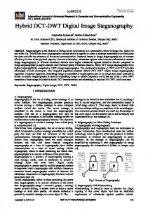
2. Biomedical imagery Three imaging modalities are utilized to test the classification system: mammography, retinal and small bowel images. Each one of these image types are used to diagnose diseases from a specific anatomical region. Although these images are quite different from one another, the current work develops a generalized framework for CAD that may be applied directly to each of the images. The only apriori assumption is a very general one: the texture between normal tissue and pathology is different. The first modality, mammography, is an imaging technology which acquires an x-ray image of the breast Ferreira & Borges (2001). They are currently the most effective method for early detection of breast cancers Cheng et al. (2006) Wei et al. (1995). A challenging problem in human-based analysis of mammography is the discrimination between malignant and benign masses. Incorrectly identifying the lesion type results in negative to positive biopsies ratios as high as 11:1 in some clinics Rangayyan et al. (1997). Normal tissue masks the lesions and breast parenchyma is much more prominent than the lesion itself Ferreira & Borges (2001). To test the CAD system with mammography images, a database is used where images contain either a benign or malignant lesion(s). Examples of benign and malignant masses (along with the contrast enhanced versionS) are shown in Figure 1. Normal regions are also shown for comparison.

Shift-Invariant DWT for Medical Image Classification

181

(a) Regular

(b) Enhanced

Fig. 1. Mammographic regions (128 × 128). (a)-(c) Normal regions, (d)-(f) circumscribed benign masses, (g)-(i) spiculated malignant masses. The contrast enhanced versions of these regions are also included to highlight the textural differences between lesions.

182


The benign masses have a rounded appearance with a defined boundary, while the inside of the mass is relatively uniform and radiolucent. This has also been noted by other others, see Ferreira & Borges (2001) Rangayyan et al. (1997) Mudigonda et al. (2000). In contrast, the malignant masses possess ill-defined boundaries, are of higher density (radiopaque) and have an overall nonuniform appearance in comparison to the benign lesions. Furthermore, spicules from malignant masses cause disturbances in the homogeneity of tissues in the surrounding breast parenchyma Rangayyan (2005). Since benign and malignant masses carry different textural qualities, these textural differences will be exploited in the CAD system. The second type of images are known as small bowel images. They are acquired by Given Imaging Ltd.’s capsule endoscopy known as the PillCamTM SB video capsule. The PillCamTM is a tiny capsule (10mm × 27mm Kim et al. (2005)), which is ingested from the mouth. As natural peristalsis moves the capsule through the gastrointestinal tract it captures video and wirelessly transmits it to a data recorder the patient is wearing around his or her waist Given Imaging Ltd. (2006a). This video provides visualization of the 21 foot long small bowel, which was originally seen as a “black box” to doctors Given Imaging Ltd. (2006b). Video is recorded for approximately eight hours and then the capsule is excreted naturally

Fig. 2. Small bowel images captured by the PillCamTM SB, which exhibit textural characteristics. (a) Healthy small bowel, (b) normal neocecal valve, (c) normal colonic mucosa, (d) normal small bowel, (e) normal jejunum, (f) small bowel polyp, (g) small bowel lymphoma, (h) GIST tumor, (i) polypoid mass, (j) small bowel polyp. with a bowel movement Given Imaging Ltd. (2006a). Clinical results for the PillCamTM show that it is a superior diagnostic method for diseases of the small intestine Given Imaging Ltd. (2006c). The downfall of this technology comes from the large amount of data which is collected while the PillCamTM - the doctor has to watch and diagnose eight hours of footage! This is quite a labourious task, which could cause the physicians to miss important clues due to fatigue, boredom or due to the repetitive nature of the task. To combat missed pathologies, the proposed CAD system could be used to double check the image data. To test out the generalized CAD system, a small bowel image database is utilized that contains both normal (healthy regions) and several abnormal images. As shown Figure 2(a)-(e), the


183

normal small bowel images contain smooth, homogeneous texture elements with very little disruption in uniformity except for folds and crevices. Many types of pathologies are found in the small bowel image database ("abnormal" image class), such as “Abnormal”: polyp, Kaposi’s sarcoma, carcinoma, etc. These diseases may occur in various sizes, shapes, orientations and locations within the gastrointestinal tract. Abnormalities have some common textural characteristics: the diseased region contains many different textured areas simultaneously and these diseased areas are composed of heterogeneous texture components. This may be seen in Figure 2(f)-(j). The data for each patient is a series of 2D colour images. As the current chapter is focused on grayscale processing, the colour images are converted to grayscale first. Additionally, each image has been lossy JPEG compressed, so feature extraction is completed in the compressed domain. Feature extraction in the compressed domain has become an important topic recently Chiu et al. (2004) Xiong & Huang (2002) Chang (1995) Armstrong & Jiang (2001) Voulgaris & Jiang (2001), since the prevalence of images stored in lossy formats far supersedes the number of images stored in their raw format. The last set of images are known as retinal images. Ophthalmologists use digital fundus cameras to acquire and collect retinal images of the human eye Sinthanayothin et al. (2003), which includes the optic nerve, fovea, surrounding vessels and the retinal layer Goldbaum (2002). Although screening with retinal imaging reduces the risk of serious eye impairment (i.e. blindness caused by diabetic retinopathy by 50% Sinthanayothin et al. (2003)), it also creates a large number of images which the doctors need to interpret Brandon & Hoover (2003). This is expensive, time consuming and may be prone to human error. The current automated system can be used to help the doctors with this diagnostic task by offering a secondary opinion of the images. The current database contains several normal (healthy) retinal images as well as several images that contain a variety of pathologies. Examples of normal and abnormal retinal images are shown in Figure 3. Healthy eyes are easily characterized by their overall homogeneous appearance, as easily seen in Figure 3(a)-(c). Eyes which contain disease do not possess uniform texture qualities. Three cases of abnormal retinal images are shown in Figure 3(d)-(f). Diabetic retinopathy, which is characterized by exudates or lesions (random whitish/yellow patches locations Wang et al. (2000)) are shown in Figure 3(a). Another clinical sign of diabetic retinopathy are microaneurysms and haemorrhages and macular degeneration, which can cause blindness if it goes untreated. Macular degeneration may be characterized by drusens, which appear as yellowish, cloudy blobs, which exhibit no specific size or shape Brandon & Hoover (2003). This is shown in Figure 3(e). These pathologies disrupt the homogeneity of normal tissues. Other diseases include central retinal vein and/or artery occlusion shown in Figure 3(f) (an oriented texture pattern which radiates from the optic nerve). 2.1 Texture for pathology discrimination

As shown in the previous subsection, pathological regions in the images have a heterogeneous appearance and normal regions are uniform. Moreover, texture elements occur at a variety of orientations, scales and locations. Thus the CAD system must be robust to all these variances, but still remain modality- or database-independent (i.e. not tuned specifically for a modality). Computing devices are becoming an integral part of our daily lives and in many times, these

184


Fig. 3. Retinal images which exhibit textural characteristics. (a)-(c) Normal, homogeneous retinal images, (d) background diabetic retinopathy (dense, homogeneous yellow clusters), (e) macular degeneration (large, radiolucent drusens with heterogeneous texture properties), (f) central retinal vein occlusion (oriented, radiating texture). algorithms are designed to mimic human behaviour. In fact, this is the major motivation of many CAD systems; to understand and analyze medical image content in the same fashion as humans do. Since texture has been shown to be an important feature for discrimination in medical images, understanding how humans perceive texture provides important clues into how a computer vision system should be designed to discriminate pathology. As shown, these images possess textural characteristics that differentiate between pathological and healthy (normal) tissues. A common denominator is that the pathological (cancerous) lesions seem to have heterogeneous, oriented texture characteristics, while the normal images are relatively homogeneous. These differences are easily spotted by the human observer and thus we want our system to also differentiate between these two texture types (homogeneity and heterogeneity) for classification purposes. To build a system that understands textural properties that is in line with human texture perception, a human texture analysis model must first be examined. When a surface is viewed, the human visual system can discriminate between textured regions quite easily. To describe how the human visual system can differentiate between textures, Julesz defined textons, which are elementary units of texture Julesz (1981). Textured regions can be decomposed using these textons, which include elongated blobs, lines, terminators and more. It was found that the frequency content, scale, orientation and periodicity of these textons can provide important clues on how humans differentiate between two or more textured areas Julesz (1981). Therefore, to create a system which mimics human understanding of texture for pathology discrimination, it is necessary that the analysis system can detect the properties of


185

the fundamental units of texture (texture markers). In accordance to Julesz’s model, textural events will be detected based on their scale, frequency and orientation.

3. Feature invariance To describe the textural characteristics of medical images, a feature extraction scheme will be used. The extracted features are fed into a classifier, which arrives at a decision related to the diagnosis of the patient. Let X ⊂ Rn represent the signal space which contains all biomedical images with the dimensions of n = N × N. Since the images X can be expected to have a very high dimensionality, using all these samples to arrive at a classification result would be prohibitive Coifman & Saito (1995). Furthermore, the original image space X is also redundant, which means that all the image samples are not necessary for classification. Therefore, to gain a more useful representation, a feature extraction operator f may map the subspace X into a feature space F f : X → F, (1)

where F ⊂ Rk , k ≤ n and a particular sample in the feature space may be written as a feature vector: F = { F1 , F2 , F2 , · · · , Fk }. If k < n, the feature space mapping would also result in a dimensionality reduction. Although it is important to choose features which provide the maximum discrimination between textures, it is also important that these features are robust. A feature is robust if it provides consistent results across the entire application domain Umbaugh et al. (1997). To ensure robustness, the numerical descriptors should be rotation, scale and translation (RST) invariant. In other words, if the image is rotated, scaled or translated, the extracted features should be insensitive to these changes, or it should be a rotated, scaled or translated version of the original features, but not modified Mallat (1998). This would be useful for classifying unknown image samples since these test images will not have structures that have the same orientation and size as the images in the training set Leung & Peterson (1992). By ensuring invariant features, it is possible to account for the natural variations and structures within the retinal, mammographic and small bowel images. As will be shown in the next section, such features are extracted from the wavelet domain. If a feature is extracted from a transform domain, it is also important to investigate the invariance properties of the transform since any invariance in this domain also translates to an invariance in the features. For instance, the 1-D Fourier spectrum is a well-known translation-invariant transform since any translation in the time domain representation of the signal, does not change the magnitude spectrum in the Fourier domain f (t − τo )⇔ F (ω ) · e− jωτo ,

(2)

for all real values of τo . Similarly, scaling in time results in a easily definable reaction in the frequency domain ω 1 ·F f (αt) ⇔ , (3) | α| α

where α is an integer value. Although the types of feature extraction algorithms that will be used have not yet been discussed, prior to designing any feature extractor, it is important to understand the necessity of robust features. The following sections will detail the analysis tool used to localize the

186


texture events, as well as the feature extraction framework that is used to extract robust features (in the RST-invariant sense).

4. Multiresolutional analysis All signals and images may be categorized into one of two categories: 1) deterministic or 2) non-deterministic (random). Deterministic signals allow for advanced prediction of signal quantities, since the signal may be described by a mathematical function. In contrast, instantaneous values of non-deterministic signals are unpredictable due to their random nature and must be represented using a probabilistic model Ross (2003). This stochastic model describes the inherent behaviour of the signal or image in question. Random signals (both 1D and 2D) may be further classified into two groups: 1) stationary or 2) nonstationary. A stationary signal (1D) is a signal which has a constant probability distribution for all time instants. As a consequence, first order statistics such as the mean and second order statistics such as variance must also remain constant. In contrast, a nonstationary signal has a time-varying probability distribution which causes quantities computed from the probability density function (PDF) to also be time-varying. For instance, the mean, variance and autocorrelation function of a nonstationary signal would change with time. Since the Fourier transform of the autocorrelation function is equal to the power spectral density (PSD) of a signal (which is related to the spectral content), the PSD of a nonstationary signal is also time-varying. Consequently, a nonstationary signal has time-varying spectral content. The medical images (as with most natural images) are nonstationary since they have spatially-varying frequency components. Texture is comprised of a variety of frequency content (and may be found in any location in the image), and therefore texture is also a type of nonstationary phenomena. Since textured regions provide important clues that discriminate between pathologies and/or healthy tissue, nonstationary analysis would add extra utility in the sense that it would quantify or localize these textural elements. As discussed, the theory of human texture perception is defined in terms of several features for texture discrimination: the scale, frequency, orientation of textons. Therefore, analyzing the scale, frequency and orientation properties of textural elements by nonstationary image analysis is in accordance to the human texture perception model. The type of nonstationary image analysis tool that will be utilized is part of the multiresolutional analysis family, and is known as the Discrete Wavelet Transform (DWT). As will be discussed, wavelet transforms are optimal for texture localization since the wavelet basis have excellent joint space-frequency resolution Mallat (1998). The section will begin by presenting the signal decomposition theory needed to understand the fundamentals of the DWT. Following the introduction, the wavelet transform (with descriptions of the wavelet and scaling basis functions) are given, with emphasis given to signal space definitions. The DWT is then defined using the filter-bank method which was implemented by the lifting-approach for the 5/3 Le Gull wavelet. 4.1 Signal decomposition techniques

Signal decomposition techniques can be used to transform the images into a representation that highlights features of interest. As such decomposition techniques are used to define the wavelet transform and its variants, some brief background is given here. A decomposition technique linearly expands a signal or image using a set of mathematical functions. For a 1D signal, using a set of real-valued expansion coefficients ak , and a series

187


of 1-D mathematical functions ψk (t) known as an expansion set (ψk (t) = ψ (t − k) for all integer values of k), a signal f (t) may be expressed as a weighted linear combination of these functions f (t) = ∑ ak · ψk (t), k ∈ Z. (4) k

If the members of the expansion set ψk (t) are orthogonal to one another:

�ψk (t), ψl (t)� = 0,

k �= l,

(5)

then it is possible to find the expansion coefficients ak ak = � f (t), ψk (t)�,

(6)

where the inner product �·� of two signals x (t) and y(t) is defined by

� x (t), y(t)� =

t

x ∗ (t) · y(t)dt.

(7)

The definition of an expansion set depends on various properties. For instance, if there is a signal f (t) which belongs to a subspace S ( f (t) ∈ S), then ψk (t) will only be called an expansion set for S if f (t) can be expressed with linear combinations of ψk (t). The expansion set forms a basis if the representation it provides is unique Burrus et al. (1998). Similarly, a basis set may be defined first and then the space S spans all functions f (t) which can be expressed by f (t) = ∑k ak · ψk (t). For images, the basis functions may be dependant on both the horizontal and vertical spatial variables ( x, y). This leads to 2D basis functions ψm,n ( x, y), where ψm,n ( x, y) = ψ ( x − n, y − m), for all (m, n ) ∈ Z. Therefore, a 2D function (image) f ( x, y), that belongs to the space of the basis functions, may be rewritten as a linear expansion f ( x, y) = ∑ ∑ am,n · ψm,n ( x, y), m n

(8)

where am,n are the 2-D expansion coefficients found by am,n = �ψm,n ( x, y), f ( x, y)�.

(9)

Using decomposition techniques, a new representation is generated. In feature extraction problems, we want this representation (i.e. coefficients ak or an,m ) to highlight the features we are interested in. This requires us to choose basis functions that are tuned to the properties of our image (i.e. nonstationary structures). While choosing which basis set to use, one of the main considerations is the functions’ space-frequency resolution. Consider the basis function ψk (t) which has an energy distribution that is concentrated near the time instant k and is spread out over the interval Δt Mallat (1998). This basis function ψk (t) 1 . Similarly, in the frequency can identify time-localized features (at k) with a resolution of Δt domain, the Fourier representation Ψξ (ω ) is concentrated in energy near the frequency ξ and spread over the interval of Δω, which captures frequency-localized features (at ξ) with a 1 resolution of Δω . Ideally, basis functions with infinitely small time and frequency would provide the best representation since time-frequency structures would be represented with infinite resolution.

188


However, this is not possible, because there is a direct trade off between time and frequency resolution of basis functions as governed by the Heisenburg uncertainty principal Burrus et al. (1998) Mallat (1998). The Heisenburg uncertainty principal states that resolution of the time-frequency functions are lower bounded by Δω · Δt ≥ 1/2.

(10)

Therefore, to capture nonstationary events with good space-frequency localization, we need basis functions that aim to operate near the theoretical lower bound. Many basis functions offer solutions, but are not optimal for all applications. For example, the Short-Time Fourier Transform (STFT) bases are not optimal because (1) they offer a fixed resolution for the entire decomposition process (thus missing features that are comprised with different scales and frequencies), (2) do not offer an easy method to access and manage the coefficients and (3) creates a drastic increase in memory consumption and computational resources. The following section will describe how the wavelet transform poses solutions to all these problems. 4.2 Wavelet transforms

The wavelet transform offers solutions to all the problems associated with other basis functions (such as the STFT) Mallat (1989) Wang & Karayiannis (1998) Vetterli & Herley (1992) Mallat (1998). It offers a multiresolutional representation (decomposes the image using various scale-frequency resolutions), which is achieved by dyadically changing the size of the window. Space-frequency events are localized with good results since the changing window function is tuned to events which have high frequency components in a small analysis window (scale) or low frequency events with a large scale Burrus et al. (1998). Therefore, texture events could be efficiently represented using a set of multiresolutional basis functions. Additionally, the discrete wavelet transform utilizes critical subsampling along rows and columns and uses these subsampled subbands as the input to the next decomposition level. For a 2-D image, this reduces the number of input samples by a factor of four for each level of decomposition. This representation may be stored back on to the original image for minimum memory usage and it also permits for an organized, computationally efficient manner to access these subbands and extract meaningful features. The wavelet transform utilizes both wavelet basis ψ j,k (t) and scaling basis φk (t) functions. The wavelet functions are used to localize the high frequency content, whereas the scaling function examines the low frequencies. The scale of the analysis window changes with each decomposition level, thus achieving a multiresolutional representation. Starting with the initial scale j = 0, the wavelet transform of any function f (t) which belongs to L2 (R) is found by f (t) =

k=∞

∑

k =− ∞

c(k) · φk (t) +

j=∞ k=∞

∑ ∑

j =0 k =− ∞

d( j, k) · ψ j,k (t),

(11)

where c(k) are the scaling or averaging coefficients (low frequency material) defined by c(k) = c0 (k) = � f (t), φk (t)� =

f (t)φk (t) dt,

(12)

189


and d j (k) are the detail wavelet coefficients (high frequency content) defined by d j (k) = d( j, k) = � f (t), ψ j,k (t)� =

f (t)ψ j,k (t) dt.

(13)

In order to achieve a wavelet transform, the functions ψ j,k (t) and φk (t) have to meet specific criteria. These criteria, the properties of the scaling/wavelet functions and the corresponding signal spaces are described next. 4.2.1 Scaling function subspaces

Consider a set of basis functions {φk (t)} which may be created by translating the prototype scaling function φ(t) Burrus et al. (1998) φk ( t ) = φ ( t − k ) , where φk (t) spans the space V o

k ∈ Z,

Vo = Spank {φk (t)}.

(14) (15)

If a set of basis functions span a signal space V o , then any function f (t) which also belongs to that space can be completely represented using those basis functions as in: f (t) = ∑k ak · φk (t) (for any f (t) ∈ Vo ). For added flexibility, the time and frequency resolution of these scaling functions may be adjusted by including an additional scale parameter j in the characteristic basis function expression (16) φj,k (t) = 2 j/2 · φ(2 j t − k), j, k ∈ Z,

where the scalar multiple 2 j/2 is included to ensure orthonormality Mallat (1989). Therefore, an entire series of basis functions can be created by simply dilating (changing the j value) or translating (changing the k value) the prototype scaling function φ(t). These basis functions span the subspace V j

V j = Spank {φk (2 j t)}, = Spank {φj,k (t)},

(17)

and any signal f (t) can be expressed using this expansion set, as long as it is also a set of V j f (t) =

∑ a k · φ (2 j t − k ), k

f (t) ∈ V j .

(18)

The introduction of a scale parameter changes the time duration of the scaling functions. This allows different resolutions to isolate different anomalies in the signals or images. For instance, if j > 0, φj,k (t) is narrower and would provide a good representation of finer detail. For j < 0, the basis functions φj,k (t) are wider and would be ideal to represent coarse information Burrus et al. (1998). 4.2.2 Wavelet basis functions

Although the scaling functions give way to a multiresolution representation, it is also necessary to investigate the spaces which span the differences of the spaces spanned by the scaling functions. These regions correspond to the high frequency details of the data.

190


...

...

Fig. 4. Nested wavelet and scaling signal spaces. The types of basis functions that can localize the details are known as wavelets ψ (t) and their corresponding signal spaces are denoted as W . Similar to scaling functions, a series of wavelet basis functions can be generated by dilating and translating the mother wavelet ψ (t) ψ j,k (t) = 2 j/2 ψ (2 j t − k),

j, k ∈ Z.

(19)

To find the mother wavelet ψ (t), it is necessary to find the relationship between the mother wavelet ψ (t) and the generating scaling function φ(t). Starting with an initial resolution of j = 0, the nested subspaces may be written as

V o ⊂ V1 ⊂ V2 ⊂ · · · ⊂ L2 .

(20)

The corresponding spaces spanned by the wavelet basis functions are shown in Figure 4, which illustrates how each W subspace spans the difference of two subspaces. As shown in Figure 4, the signal spaces V1 and V2 may be expressed as

and

V1 = V o ⊕ W o ,

(21)

V2 = V o ⊕ W o ⊕ W1 ,

(22)

where ⊕ is a direct sum. If V j is the space spanned by the scaling functions φj,k (t) and V j+1 is the space spanned by the functions φj+1,k (t), then W j is the disjoint difference or the orthogonal compliments of V j and V j+1 spanned by the wavelet basis functions ψ j,k (t). This may be shown by V j+1 = V j ⊕ W j , ∀ j ∈ Z. (23)

Using Equation 21, Equation 22 and Figure 4, a general expression for the L2 subspace may be developed: L 2 = V o ⊕ W o ⊕ W1 ⊕ W2 ⊕ · · · , (24)

and since these subspaces are orthogonal to one another

V o ⊥ W o ⊥ W1 ⊥ W2 ⊥ W3 · · · ,

(25)

191


the corresponding basis functions which span these spaces are also orthogonal

�φj,k (t), ψ j,k (t)� =

φj,k (t) · ψ j,k (t)dt = 0.

(26)

Furthermore, wavelet spaces at a scale j are a subset of the scale spaces at the next scale j + 1

W j ⊂ V j +1 .

(27)

Consequently, wavelets reside in the space spanned by the next narrower scaling function and can be expressed as a weighted sum of shifted scaling functions, φ(2t) √ ψ (t) = ∑ h1 (n ) · 2 · φ(2t − n ), n ∈ Z, (28) n

where h1 (n ) are the wavelets’ coefficients. Equation 28 shows that the generating wavelet ψ (t) can be produced from the prototype scaling function φ(t) by choosing the appropriate h1 (n ). In order to ensure orthogonality, the scaling and wavelet coefficients must be related by Burrus et al. (1998) h1 (n ) = (−1)n ho (1 − n ). (29) Therefore, for analysis with orthogonal wavelets, the highpass filter h1 (n ), which is half-band, is calculated as the quadrature mirror filter of the lowpass ho (n ). These filters may be used to efficiently implement the wavelet transform for discrete signals (the Discrete Wavelet Transform) and is discussed next. 4.3 Discrete wavelet transform

In order to perform the wavelet transform for discrete images, implementation of the DWT using filterbanks is popular choice since the complexities of the wavelet transform are explained in terms of filtering operations (which is intuitive). The material is first presented for one dimensional signals and then is expanded to 2D for images. After performing a series of simplifications and change of variables Burrus et al. (1998) Mallat (1998) Vetterli & Herley (1992), Equation 28 may be rewritten as c j (k) = ∑ ho (m − 2k)c j+1 (m),

(30)

d j (k) = ∑ h1 (m − 2k)c j+1 (m).

(31)

m

and

m

This illustrates that c j (k) and d j (k) can be found by filtering c j+1 (k) with ho and h1 , respectively, followed by a decimation by a factor of 2. The two filters, ho (n ) and h1 (n ) are half-band lowpass and highpass filters, respectively. Consequently, the lowpass filter ho (n ) produces lowpassed or averaged coefficients c j (k) and the highpass filter h1 (n ) creates highpassed or detail coefficients d j (k). To compute the DWT coefficients for two levels, examine the two stage analysis filterbank in Figure 5(a) alongside the signal spaces in Figure 5(b). Note that the initial scale here is j + 1, and therefore c j+1 would represent the original input signal. After one level of decomposition, the lowpass coefficients c j and the highpass details d j are produced. For a multiresolutional representation, c j are further decomposed with ho and h1 , to produce the coefficients c j−1 (k)

192


and d j−1 (k) (they describe the next scale of low and high frequency structures). The 2D extension for images is detailed next.

Fig. 5. (a) Computing the 1-D wavelet and scaling coefficients using filtering and decimation with a 2-stage analysis filterbank, (b) corresponding decomposition tree showing the division of signal spaces. 4.3.1 2-D extension for images

Instead of having a wavelet or filter which is a function of the two spatial dimensions of an image, the filter can be separable, which allows a particular 1D filter to be applied to the rows and columns of an image separately to gain the desired overall 2D response Lawson & Zhu (2004). A separable filter for two dimensions may be denoted by: H ( z1 , z2 ) = H ( z1 ) · H ( z2 ),

(32)

where z1 and z2 relate to the spatial dimensions of an image. Therefore, the filters defined for the 1D DWT may be applied separably to gain a 2D DWT representation for images. The 2-D DWT filterbank scheme for an N × N image x (m, n ) is shown in Figure 6. Initially, the filters Ho (z) and H1 (z) are applied to the rows of image x (m, n ), creating two images which respectively contain the low and high frequency content of the image in question. After this, both frequency bands are subsampled by a factor of 2, and are sent to the next set of filters for filtering along the columns. After these bands have been filtered, decimation by a factor of 2 is again performed, but this time along columns. At the output of one level of decomposition, as shown in Figure 6, there are four subband images of size N2 × N 2 labeled LL, LH, HL and HH. Using the separability concept, at scale j, these subbands may be computed by LL j ( x, y) =

∑ ∑ ho (m − 2x)ho (n − 2y) · LL j+1 (m, n),

(33)

HL j ( x, y) =

∑ ∑ ho (m − 2x)h1 (n − 2y) · LL j+1 (m, n),

(34)

LH j ( x, y) =

∑ ∑ h1 (m − 2x)ho (n − 2y) · LL j+1 (m, n),

(35)

HH j ( x, y) =

∑ ∑ h1 (m − 2x)h1 (n − 2y) · LL j+1 (m, n).

(36)

m n m n m n m n


193

The first letter of the subimages indicates the operation that was performed on the columns (i.e. L is for lowpass filtering with Ho (z) and H is for highpass filtering with H1 (z)) whereas the last letter indicates which operation was performed on the rows. If more levels

Fig. 6. Filterbank implementation of 2-D discrete wavelet transform (DWT). of decomposition are required, the LL band may be recursively reapplied to the analysis filterbank of Figure 6. For two levels of decomposition, the placement of the coefficients back onto the image is shown in Figure 7. To examine the localization properties of the 2D DWT, consider Figure 8. The edges and

Fig. 7. Graphical depiction of wavelet coefficient placement for two levels of decomposition. corners of the square (the original image) are composed of localized high frequency content, which is captured in the high frequency subbands in the wavelet domain, regardless of the orientation (horizontal, diagonal, vertical). As texture is comprised of such localized high frequency events, utilization of such a transform will be able to describe the textural events as required. The diffusion of textural features or events will occur across subbands, which

194


allows features to be captured not only within subbands, but also across subbands. For an example of the localization properties of wavelets in a medical image, as well as the textural differences between normal and abnormal medical images, see Figure 9. The normal image’s decomposition exhibits an overly homogeneous appearance of the wavelet coefficients in the HH, HL and LH bands (which reflects the uniform nature of the original image). The decomposition of the retinal image with diabetic retinopathy shows that each of the higher frequency subbands localizes the retinopathy, which appears as heterogeneous textured blobs (high-valued wavelet coefficients) in the center of the subband. This illustrates how the DWT can localize the textural differences in medical images also how multiscale texture may be used to discriminate between pathological cases . Similar results are obtained with the small bowel and mammographic lesions, however, are not shown here due to space constraints. Another benefit of wavelet analysis is that the basis functions are scale-invariant.

Fig. 8. Left: original image. Right: one level of DWT of left image. Scale-invariant basis functions will give rise to a localized description of the texture elements, regardless of their size or scale, i.e. coarse texture can be made up of large textons, while fine texture is comprised of smaller elementary units. Therefore, the DWT can handle both of these scenarios. Although the filterbank method is efficient, it requires a lot of filtering operations which is computationally expensive. For more efficient implementations of the filterbank-based DWT, the lifting-based approach is one such approach that is employed in the current framework and detailed next. 4.4 Lifting-based DWT

To compute the DWT in an efficient manner, the lifting based approach is used Fernández et al. (1996) Sweldens (1995) Sweldens (1996). To increase computation speed, lifting based approaches make optimal use of similarities which exist between the lowpass (H1 (z)) and highpass (Ho (z)) filters. All 1D implementations will be later extended to 2D implementations by ’lifting’ both the columns and the rows separately. The lifting based DWT is an efficient scheme since it aims to implement complicated functions with simple and invertible stages Zhang & Zeytinoglu (1999). Compared to the filterbank method, the lifting based DWT method offers a less computationally expensive solution to compute the DWT Zhang & Zeytinoglu (1999) Sweldens (1996). The lifting based scheme relies on three operations to achieve the discrete wavelet transform:


195

Fig. 9. One level of DWT decomposition of retinal images. Left: normal image decomposition. Right: decomposition of retinal image with diabetic retinopathy. Contrast enhancement was performed in the higher frequency bands (HH, LH, HL) for visualization purposes. 1) split, 2) predict and 3) update. These three operations which comprise the 1-D lifting scheme, are shown in Figure 10, where S is the splitting function, P is the predictor function and U is the update operation. As shown by Figure 10, the scaling and wavelet coefficients (c j (n ) and d j (n )) are still from the previous level’s coefficients, c j+1 (n ). Lifting may be also applied separably to the rows and columns of an image to arrive at a 2D DWT.

Fig. 10. Generalized 1-D lifting based implementation of the DWT. 4.4.1 Splitting

The splitting operation divides the 1-D input string into even and odd samples, as denoted by c j+1 (2n ) and c j+1 (2n + 1), respectively. Using digital signal processing, the even samples may be obtained by decimating the original signal by a factor of 2, and the odd samples may be obtained by subsampling a time shifted (single unit of time) version of the original signal by 2. This is often referred to as the Lazy Wavelet Transform Fernández et al. (1996).

196


4.4.2 Prediction

In order to compute the wavelet coefficients d j (n ), a lifting scheme uses a predictor to interpolate the odd-indexed coefficients from the previous scale (c j+1 (2n + 1)). The prediction is subtracted from the original odd-indexed signal to produce the wavelet coefficients d j (n ). This may expressed as d j (n ) = c j+1 (2n + 1) − P (c j+1 (2n + 1)),

(37)

where P(·) is the predictor function. As stated earlier, the wavelet coefficients correspond to the high frequency components which makes this operation equivalent to highpass filtering. A good predictor function would produce small valued wavelet coefficients (ideally zero), since the predicted version of the signal would be identical to the original. However, for nonstationary signals (such as biomedical images) that have properties which change over time, it is not possible to exactly predict the signal Zhang & Zeytinoglu (1999) and non-zero wavelet coefficients can be expected. There are many different predictor functions which may be used Maragos et al. (1984) Haijiang et al. (2004) Denecker et al. (1997), however, in order to implement the forward wavelet transform, the interpolation function is chosen such that it relates to the wavelet ψ (t) Zhang & Zeytinoglu (1999). 4.4.3 Updating

In a lifting based DWT implementation, the scaling coefficients c j (n ) are computed as the sum of the even-indexed samples (c j+1 (2n )) and an updated version of the wavelet coefficients d j (n ) as shown below: c j (n ) = c j+1 (2n ) + U (d j (n )), (38) where U (·) is the update function. This operation isolates the low frequency components within the original signal. For images, lifting based DWT must be extended to two dimensions. As shown earlier in the 2D DWT filterbank approach, 1D wavelet transforms were applied separably to the images in order to gain a 2D DWT representation. This also applies to lifting based schemes as well. By sequentially applying the lifting operation first to the rows and then to the columns of an image, the forward transformation is achieved. The forward operation is depicted in Figure 11.

Fig. 11. Lifting-based implementation of the DWT for two dimensional signals.


197

4.5 5/3 Wavelet

The integer wavelet which will be used is part of the Odd-Length Analysis/Synthesis Filter (OLASF) family, where the number of filter taps in the FIR filter (for the filterbank implementation) are odd Adams & Ward (2003). Additionally, biomedical images are high resolution images, which results in large image sizes. Consequently, for these large-sized images, a wavelet with fewer taps is desired so that the overall computational load may be reduced. The 5/3 Le Gull wavelet will be used since the filter lengths are small (5 and 3 taps for the analysis low and highpass filters) and can warrant an efficient implementation Marcellin et al. (2000) Zhang & Fritts (2004) . The 5/3 filter coefficients are listed in Table ??.

i 0 ±1 ±2

Analysis Coefficients Synthesis Coefficients h o (i ) h1 (i ) h o (i ) h1 (i ) + 86 +1 +1 + 86 + 82 − 12 − 21 + 82 − 81 + 81

Table 1. Analysis and synthesis filter coefficients for the 5/3 wavelet. Using the 5/3 integer wavelet, the highpass details d j (n ) can be computed using a lifting based approach: c j+1 (2n ) + c j+1 (2n + 2) , (39) d j (n ) = c j+1 (2n + 1) − 2 where � X � is the greatest integer less than or equal to X. The low frequency, average coefficients c j (n ) may be found using an update function c j (n ) = c j+1 (2n ) +

d j ( n ) + d j ( n − 1) + 2 . 4

(40)

For reconstruction, the reverse DWT can be found by reversing the arithmetic operations of the forward transform. This is shown below: d j ( n ) + d j ( n − 1) + 2 c j+1 (2n ) = c j (n ) + , (41) 4 c j+1 (2n ) + c j+1 (2n + 2) c j+1 (2n + 1) = d j (n ) − . (42) 2 These equations may be applied separably to the images in order to gain a 2-D DWT representation.

5. Shift-invariant discrete wavelet transform Although the DWT is scale-invariant, it is well known that the DWT is shift-variant Mallat (1998), i.e. the coefficients of a circularly shifted image are not translated versions of the

198


original image’s coefficients. For instance, the DWT of an input biomedical image f ( x, y) can be shown as: f ( x, y) −→ DWT −→ F(k1 , k2 , j )

where F(k1 , k2 , j ) are the 2-D DWT coefficients at scale j. A shift of the image will result in a different set of coefficients �

� � f ( x + Δx, y + Δy) −→ DWT −→ F(k1 , k2 , j ) �

where k1 �= k1 + a1 · Δx and k2 �= k2 + a2 · Δy for ( a1 , a2 ), (Δx, Δy) ∈ Z, indicating that the two sets of coefficients are not translated versions of one another. Shift-variance causes significant challenges in a feature extraction problem. For example,

Fig. 12. Image (simulated benign lesion). consider the image of Figure 12 (the center circle can be considered as a circumscribed benign lesion, or something to that effect). If this circle is translated by a small amount (which is equivalent to the lesion being located in different regions of an image), the extracted features would be different. To illustrate this, the image in Figure 12 is translated by shifts of (Δx, Δy) = {(0,0), (0,1), (1,0), (1,1)} and for each translation, the DWT is performed. Then, the mean and variance of the wavelet coefficients are extracted from the LH band (moments are RST invariant, so any invariance would be a consequence of the transform). The extracted features are shown in Table 2. As shown by these results, images with pathology (texture) located in different regions of the images would result in different feature sets, thus leading to high misclassification results. For shift-invariant features, it is necessary to utilize a shift-invariant discrete wavelet Input shift (Δx, Δy) (0,0) (0,1) (1,0) (1,1)

Mean μ Variance σ2 -0.050537 97.017 -0.051025 100.42 0.057861 96.82 0.058350 98.383

Table 2. Mean μ and variance σ2 of the DWT coefficients of the LH band for circular translates (Δx, Δy) of Figure 12. transform (SIDWT) on the input image f ( x, y) f ( x, y) −→ SIDWT −→ F(k1 , k2 , j )


199

to compute the wavelet coefficients F(k1 , k2 , j ). The representation achieved by such a transform would be considered shift-invariant if a shift of the input image (Δx, Δy) ∈ Z results in output coefficients which are exactly the same as F(k1 , k2 , j ), or a spatially shifted version of it. This may be shown by �

� � f ( x + Δx, y + Δy) −→ SIDWT −→ F(k1 , k2 , j ) �

where k1 = k1 + b1 · Δx and k2 = k2 + b2 · Δy for some (b1 , b2 ) ∈ Z. If the coefficients are exactly the same: b1 = b2 = 0. The shift-variant property of the DWT is widely known and several solutions have been proposed. Mallat et. al use an overcomplete, redundant dictionary, which corresponds to filtering without decimation Mallat (1998) Bradley (2003). From the filtered and fully sampled version of the image, local extrema are used for translation invariance since a shift in the input image results in a corresponding shift of the extrema Mallat (1998) Liang & Parks (1994). Since there is no decimation, each level of decomposition contains as many samples as the input image, thus making the algorithm computationally complex. It also requires significant memory bandwidth. Simoncelli et. al propose an approximate shift-invariant DWT algorithm by relaxing the critical sampling requirements of the DWT Simoncelli et al. (1992). This algorithm is known as the power-shiftable DWT since the power in each subband remains constant. As explained in Bradley (2003), the shift-variant property is also related to aliasing caused by the DWT filters. The power shiftable transform tries to remedy this problem by reducing the aliasing of the mother wavelet in the frequency domain. The modifications to the mother wavelet result in a loss of orthogonality Liang & Parks (1998). The Matching Pursuit (MP) algorithm can also achieve a shift-invariant representation, when the decomposition dictionary contains a large amount of redundant wavelet basis functions Mallat & Zhang (1993). However, the MP algorithm is extremely computationally complex and arriving at a transformed representation causes significant delays Cohen et al. (1997). Bradley combines features of the DWT pyramidal decomposition with the a` trous algorithm Mallat (1998), which provides a trade off between sparsity of the representation and time-invariance Bradley (2003). Critical sampling is only carried out for a certain number of subbands and the rest are all fully sampled. This representation only achieves an approximate shift-invariant DWT Bradley (2003). The algorithms discussed either try to minimize the aliasing error by relaxing critical subsampling and/or add redundancy into the wavelet basis set. However, these algorithms either suffer from lack of orthogonality (which is not always an issue for feature extraction), achieve an approximate shift-invariant representation, are computationally complex or require significant memory resources. To combat these downfalls, the SIDWT algorithm proposed by Beylkin, which computes the DWT for all circular shifts in a computationally efficient manner Beylkin (1992) is utilized. The proposed SIDWT utilizes orthogonal wavelets, thereby resulting in less redundancy in the representation Liang & Parks (1994), and a more efficient implementation. Belkyn’s work has also been extended to 2-D signals by Liang et. al Liang & Parks (1994) Liang & Parks (1998) Liang & Parks (1996) and its performance in a biomedical image feature extraction application will be investigated.

200


5.1 2D SIDWT algorithm

For different shifts of the input image, it was shown that the DWT can produce one of four possible representations after one level of decomposition. These four DWT coefficient sets (cosets) are not translated versions of one another and each coset may be generated as the DWT response to one of four shifts of the input: (0, 0), (0, 1), (1, 0), (1, 1), where the first index corresponds to the row shift and the second index is the column shift. All other shifts of the input (at this decomposition level) will result in coefficients which are shifted versions of one of these four cosets. Therefore, to account for all possible representations, these four cosets may be computed for each level of decomposition. This requires the LL band from each level to be shifted by the four translates {(0, 0), (0, 1), (1, 0), (1, 1)} and each of these new images to be separately decomposed to account for all representations. To compute the coefficients at the jth decomposition level, for the input shift of (0, 0), the subbands LL j , LH j , HL j , HH j may be found by filtering the previous levels coefficients LL j+1 , as shown below: j

LL (0,0) ( x, y) = j

LH(0,0) ( x, y) = j

HL (0,0) ( x, y) = j

HH(0,0) ( x, y) =

∑ ∑ ho (m − 2x)ho (n − 2y) · LL j+1(m, n),

(43)

∑ ∑ h1 (m − 2x)ho (n − 2y) · LL j+1(m, n),

(44)

∑ ∑ ho (m − 2x)h1 (n − 2y) · LL j+1(m, n),

(45)

∑ ∑ h1 (m − 2x)h1 (n − 2y) · LL j+1 (m, n).

(46)

m n m n m n m n

The subband expressions listed in Equation 43 through to Equations 46 contain the coefficients which would appear the same if LL j+1 is circularly shifted by {0, 2, 4, 6, · · · , s} rows and {0, 2, 4, 6, · · · , s} columns, where s is the number of row and column coefficients in each of the subbands for the level j + 1. The subband coefficients which are the response to a shift of (0,1) in the previous level’s coefficients may be computed by j

LL (0,1) ( x, y) = j

LH(0,1) ( x, y) = j

HL (0,1) ( x, y) = j

HH(0,1) ( x, y) =

∑ ∑ ho (m − 2x)ho (n − 2y) · LL j+1 (m, n − 1),

(47)

∑ ∑ h1 (m − 2x)ho (n − 2y) · LL j+1 (m, n − 1),

(48)

∑ ∑ ho (m − 2x)h1 (n − 2y) · LL j+1 (m, n − 1),

(49)

∑ ∑ h1 (m − 2x)h1 (n − 2y) · LL j+1(m, n − 1),

(50)

m n m n m n m n

which contain all the coefficients for {0, 2, 4, 6, · · · , s} row shifts and {1, 3, 5, 7, · · · , s − 1} column shifts of LL j+1 . Similarly, for a shift of (1,0) in the input, the DWT coefficients may be found by j

LL (1,0) ( x, y) = j

LH(1,0) ( x, y) =

∑ ∑ ho (m − 2x)ho (n − 2y) · LL j+1 (m − 1, n),

(51)

∑ ∑ h1 (m − 2x)ho (n − 2y) · LL j+1 (m − 1, n),

(52)

m n m n

201


j

HL (1,0) ( x, y) = j

HH(1,0) ( x, y) =

∑ ∑ ho (m − 2x)h1 (n − 2y) · LL j+1 (m − 1, n),

(53)

∑ ∑ h1 (m − 2x)h1 (n − 2y) · LL j+1(m − 1, n),

(54)

m n m n

which contain all the coefficients if the previous levels’ coefficients LL j+1 are shifted by {1, 3, 5, 7, · · · , s − 1} rows and {0, 2, 4, 6, · · · , s} columns. For an input shift of (1,1), the subbands may be computed by j

LL (1,1) ( x, y) = j

LH(1,1) ( x, y) = j

HL (1,1) ( x, y) = j

HH(1,1) ( x, y) =

∑ ∑ ho (m − 2x)ho (n − 2y) · LL j+1(m − 1, n − 1),

(55)

∑ ∑ h1 (m − 2x)ho (n − 2y) · LL j+1 (m − 1, n − 1),

(56)

∑ ∑ ho (m − 2x)h1 (n − 2y) · LL j+1 (m − 1, n − 1),

(57)

∑ ∑ h1 (m − 2x)h1 (n − 2y) · LL j+1 (m − 1, n − 1).

(58)

m n m n m n m n

Similarly, these subband coefficients account for all DWT representations, which correspond to {1, 3, 5, 7, · · · , s − 1} row shifts and {1, 3, 5, 7, · · · , s − 1} column shifts of the input subband LL j+1 . Performing a full decomposition will result in a tree which contains the DWT coefficients for all N 2 circular translates of an N × N image. At each level of decomposition, the LL band is shifted four times, and for each shift (0, 0), (0, 1), (1, 0), (1, 1), four new sets of subbands are generated. The decomposition tree is shown in Figure 13 and each circular node corresponds to only three subband images: HH, LH and HL, since at each level the LL band is shifted and then further decomposed. The number of coefficients in each node (per decomposition level) remains constant at 3N 2 , and a complete decomposition tree will have N 2 (3log2 N + 1) elements Liang & Parks (1994). To compute the DWT for all N 2 translates of the image costs O( N 2 log2 N ), due to the periodicity of the rate change operators Liang & Parks (1998). To achieve shift-invariance, a subset of the wavelet coeffieints in the Tree of Figur e13 must be chose in a consistent manner. To do this, metrics can be computed from the tree. This requires an organized way to address each of the coefficients. A proper addressing scheme will help to find the wavelet transform for a particular translate (m, n ), where m is the row shift and n is the column translate of the input image. For a path in the tree, which originates from the root, terminates at a leaf node and corresponds to the translate (m, n ), an expression may be developed which considers all row shifts and all column shifts as binary vectors, where each vector entry can be either 0 or 1. Therefore, the binary expansions may be rewritten as m=

log2 N

∑

i =1

n=

log2 N

∑

i =1

a i 2i − 1 ,

(59)

b i 2i − 1 ,

(60)

202


…..

…..

…..

…..

…..

Fig. 13. Shift-invariant DWT decomposition tree for three decomposition levels. where ai and bi correspond to the binary symbol which represents the row and column shift at decomposition level i, respectively. In order to find the three subimages (HL, HH and LH) which correspond to the translate (m, n ) in the K th decomposition level in the tree, it is necessary to find the S th node which corresponds to this shift, as shown below S = 2·

K

K

i =1

i =1

∑ a i 4K − i + ∑ b i 4K − i .

(61)

After the three subimages are located within the tree, to ensure that they correspond to the translate of the input by (m, n ), these three images (HH, LH, HL) must be shifted by (xShift, yShift) xShift =

log2 N

∑

i = K +1

yShift =

log2 N

∑

i = K +1

a i 2i − K − 1 ,

(62)

b i 2i − K − 1 .

(63)

This scheme allows us to address the wavelet coefficients that correspond to a particular shift of the input. The following section, which focuses on Coifmen and Wickenhauser’s best basis selection technique Coifman & Wickerhauser (1992), is focused on a method to select a consistent set of wavelet coefficients which are independent of the input translation. Since the same coefficients are selected every time the algorithm is run, regardless of any initial offset, shift-invariance is achieved.

203


5.2 Best basis paradigm

Coifmen and Wickerhauser defined a method to choose a set of basis functions, based on the minimization of a cost function J Coifman & Wickerhauser (1992). The cost function J is often called an “information cost” and it evaluates and compares the efficiency of many basis sets Coifman & Saito (1995). Although there are many choices for cost functions, an additive information cost is preferred so that a fast-divide and conquer tree search algorithm may be used to find the best set of wavelet coefficients Liang & Parks (1994). A cost function J is additive if it maps a sequence { xi } to R while ensuring that the following properties are always true:

J (0) = 0,

J ({ xi }) =

∑ J ( x i ).

(64) (65)

i

To choose a consistent set of wavelet coefficients, an entropy cost function J is used for best basis determination. Entropy gives insight about the uniformity of the coefficients’ representation (maximum energy compaction), which may be used for texture analysis. Furthermore, entropy is beneficial since it can achieve additivity Coifman & Saito (1995). Shown below is the expression of entropy which is minimized: hr ( x ) =

∑ | xi |r log| xi |r ,

(66)

i

where r is usually set to 1 or 2. To choose the best basis representation, we begin at the bottom of the decomposition tree (see

Fig. 14. Best basis selection corresponding to the minimum cost path. Figures 13 and 14) and work upwards. For each parent node, there are four child nodes, each containing the high frequency subbands of a particular translate. The cost A of a particular translate ( p, q ) ∈ {(0, 0), (0, 1), (1, 0)(1, 1)} at some node is computed by summing the cost of the individual high frequency subbands for that shift:

A( p,q) = J ( LH( p,q) ) + J ( HL ( p,q) ) + J ( HH( p,q) ).

(67)

204


To minimize entropy, the node with the minimum cost for each parent would be selected at every decomposition level. The path which is connected from the root of the tree all the way down to the leaves, is selected as the the minimum cost path, as shown in Figure 14. This path corresponds to the DWT of a particular translate and is chosen as the consistent set of basis functions in order to achieve shift-invariance.

6. Multiscale texture analysis Now that a transformation has been employed which can robustly localize the scale-frequency properties of the textured elements in the medical images, it is important to design an analysis scheme which can quantify such textured events. To do this, this work proposes the use of a multiscale texture analysis scheme. Extracting features from the wavelet domain will result in a localized texture description, since the DWT has excellent space-localization properties. To extract texture-based features, normalized graylevel cooccurrence matrices (GCMs) are employed in the wavelet domain. GCMs count the the number of two-pixel combinations and are typically normalized so that the matrix may be treated as a probability density function (PDF). In the wavelet domain, each entry of the normalized GCM is represented as p (l1 , l2 , d, θ ) =

P ( l1 , l2 ) , L −1 L −1 ∑ l1 =0 ∑ l2 =0 P ( l 1 , l 2 )

(68)

where P (l1 , l2 ) is the number of occurrences of wavelet coefficients l1 and l2 at a distance d and angle θ. Additionally, ∑l1 ∑l2 P (l1 , l2 ) is the normalizing factor and L is the maximum number of graylevels in the image. Note that these matrices are symmetric: p (l1 , l2 , d, θ ) = p (l2 , l1 , d, θ ). In the wavelet domain, GCMs are computed for adjacent wavelet coefficients. Such a second order PDF examines the correlation or relationship of wavelet coefficients to one another. Since texture is captured by the multiresolutional analysis scheme (large valued coefficients for edgy regions in a variety of scales), wavelet-based GCMs describe the statistical nature of the texture in our image. As texture is localized in a variety of directions, the GCMs are computed for each scale j at several angles θ. They are computed at multiple angles and scales since orientation and scale is play an important role in texture discrimination. In the wavelet domain, each subband isolates different frequency components - the HL band isolates horizontal edge components, the LH subband isolates horizontal edges, the HH band captures the diagonal high frequency components and LL band contains the lowpass filtered version of the original. Consequently, to capture these oriented texture components, the GCM is computed at 0◦ in the HL band, 90◦ in the LH subband, 45◦ and 135◦ in the HH band and 0◦ , 45◦ , 90◦ and 135◦ in the LL band to account for any directional elements which may still may be present in the low frequency subband. Moreover, d = 1 for fine texture analysis. From these GCMs, homogeneity h and entropy e are computed for each decomposition level using Equation 69 and 70. Homogeneity (h) describes how uniform the texture is and entropy (e) is a measure of nonuniformity or the complexity of the texture. h(θ ) =

L −1 L −1

∑ ∑

l1 =0 l2 =0

p2 (l1 , l2 , d, θ )

(69)

205


e(θ ) = −

L −1 L −1

∑ ∑

l1 =0 l2 =0

p (l1 , l2 , d, θ ) log2 ( p (l1 , l2 , d, θ ))

(70)

These features describe the relative uniformity of textured elements in the wavelet domain (which are localized with good results due to the space-frequency resolution of the bases). Recall that abnormal and normal cases were shown to have significant differences in terms of their texture uniformity (normal images contained smooth texture while abnormal images were heterogeneous). Therefore, such a scheme, which captures textural differences between images, should be able to arrive at high classification results for CAD (i.e. the classification of normal and abnormal retinal and small bowel images, and differentiation between malignant and benign lesions in the mammogram images). For each decomposition level j, more than one directional feature is generated for the HH and LL subbands. The features in these subbands are averaged so that: features are not biased to a particular orientation of texture and the representation will offer some rotational invariance. The features generated in these subbands (HH and LL) are shown below (note that the quantity in parenthesis is the angle at which the GCM was computed): 1 j j j hHH = hHH (45◦ ) + hHH (135◦ ) , 2 1 j j j eHH = eHH (45◦ ) + eHH (135◦ ) , 2 1 j j j j j hLL = hLL (0◦ ) + hLL (45◦ ) + hLL (90◦ ) + hLL (135◦ ) , 4 1 j j j j j eLL = eLL (0◦ ) + eLL (45◦ ) + eLL (90◦ ) + eLL (135◦ ) . 4

As a result, for each decomposition level j, two feature sets are generated: j j j j j hHH , hLL , Fh = hHL (0◦ ), hLH (90◦ ), j j j j j eHH , eLL , Fe = eHL (0◦ ), eLH (90◦ ),

(71) (72)

j j j j hLL , eHH and eLL are the averaged texture descriptions from the HH and LL where hHH , j

j

j

j

band previously described and hHL (0◦ ), eHL (0◦ ), hLH (90◦ ) and eLH (90◦ ) are homogeneity and entropy texture measures extracted from the HL and LH bands. Since directional GCMs are used to compute the features in each subband, the final feature representation is not biased for a particular orientation of texture and may provide a semi-rotational invariant representation.

7. Classification After the multiscale texture features have been extracted, a pattern recognition technique is needed classify the features. A large number of test samples are required to evaluate a classifier with low error (misclassification) rates since a small database will cause the parameters of the classifiers to be estimated with low accuracy. This requires the biomedical image database to be large, which may not always be the case since acquiring the images for specific diseases can take years. If the extracted features are strong (i.e. the features are mapped into nonoverlapping clusters in the feature space) the use of a simple (linear)

206


classification scheme will be sufficient in discriminating between classes. The desire is to test the robustness of the found feature set to the variations found in image databases. This can be easily determined by a linear classifier. To satisfy the above criteria, linear discriminant analysis (LDA) will be the classification scheme used in conjunction with the Leave One Out Method (LOOM). In LOOM, one sample is removed from the whole set and the discriminant functions are derived from the remaining N − 1 data samples and the left out sample is classified. This procedure is completed for all N samples. LOOM will allow the classifier parameters to be estimated with least bias Fukunaga & Hayes (1989).

8. Results The objective of the proposed system is to automatically classify pathologies based on their textural characteristics. Such a system examines texture in accordance to the human texture perception model and is shown in Figure 15.

Fig. 15. System block diagram for the classification of medical images. The classification performance of the proposed system is evaluated for three types of imagery: 1. Small Bowel Images: 41 normal and 34 abnormal (submucosal masses, lymphomas, jejunal carcinomas, multifocal carcinomas, polypoid masses, Kaposi’s sarcomas, etc.), 2. Retinal Images: 38 normal, 48 abnormal (exudates, large drusens, fine drusens, choroidal neovascularization, central vein and artery occlusion, arteriosclerotic retinopathy, histoplasmosis, hemi-central retinal vein occlusion and more), 3. Mammograms: 35 benign and 19 malignant lesions. The image specifications are shown in Table 3 and example images were shown earlier in Section 2. Only the luminance plane was utilized for the colour images (retinal and small bowel), in order to examine the performance of grayscale-based features. Furthermore, in the mammogram images, only a 128 × 128 region of interest is analyzed which contains the candidate lesion (to strictly analyze the textural properties of the lesions). Features were Small Bowel Colour (24 bpp) Lossy (.jpeg) 256 × 256

Retinal Colour (24 bpp) Lossy (.jpeg) 700 × 605

Mammogram Grayscale (8 bpp) Raw (.pgm) 1024 × 1024

Table 3. Medical image specifications extracted from the higher levels of decomposition (the last three levels were not included as further decomposition levels contain subbands of 8×8 or smaller, resulting in skewed j j probability distribution (GCM) estimates). Therefore, the extracted features are Fe and Fh for j = {1, 2, · · · , J }, where J is the number of decomposition levels minus three.

207


In order to find the optimal sub-feature set, an exhaustive search was performed (i.e. all possible feature combinations were tested using the proposed classification scheme). For the small bowel images, the optimal classification performance was achieved by combining homogeneity features from the first and third decomposition levels with entropy from the first decomposition level (see Khademi & Krishnan (2006) for more details): h1HH , h1LL , (73) Fh1 = h1HL (0◦ ), h1LH (90◦ ), Fh3 = h3HL (0◦ ), h3LH (90◦ ), h3HH , h3LL , (74) e1HH , e1LL , . (75) Fe1 = e1HL (0◦ ), e1LH (90◦ ),

The optimal feature set for the retinal images were found to be homogeneity features from the fourth decomposition level with entropy from the first, second and fourth decomposition levels (see Khademi & Krishnan (2007) for more details): h4HH , h4LL , (76) Fh4 = h4HL (0◦ ), h4LH (90◦ ), e1HH , e1LL , Fe1 = e1HL (0◦ ), e1LH (90◦ ), (77) Fe2 = e2HL (0◦ ), e2LH (90◦ ), e2HH , e2LL , (78) Fe4 = e4HL (0◦ ), e4LH (90◦ ), e4HH , e4LL , . (79) Lastly, the optimal feature set for the mammographic lesions were found by combining homogeneity features from the second decomposition level with entropy from the fourth decomposition level: Fh2 = h2HL (0◦ ), h2LH (90◦ ), h2HH , h2LL , (80) e4HH , e4LL . . (81) Fe4 = e4HL (0◦ ), e4LH (90◦ ), Using the above features in conjunction with LOOM and LDA, the classification results for the small bowel, retinal and mammogram images are shown as a confusion matrix in Table 4, Table 5 and Table 6, respectively. Normal Abnormal

Normal 35 (85%) 5 (15%)

Abnormal 6 (15%) 29 (85%)

Table 4. Results for small bowel image classification.

Normal Abnormal

Normal 30 (79%) 7 (14.6%)

Table 5. Results for retinal image classification.

Abnormal 8 (21%) 41 (85.4%)

208


Benign Malignant

Benign 28 (80%) 8 (42%)

Malignant 7 (20%) 11 (58%)

Table 6. Results for mammogram ROI classification.

9. Conclusions A total of 75 abnormal and normal bowel images were correctly classified at an average rate of 85%, 86 retinal images had an average classification accuracy of 82.2% and the mammogram lesions (54) were classified correctly 69% on average. The classification results are quite high, considering that the system wasn’t tuned for a specific modality. The system performed well, even though: (1) pathologies came in various orientations, (2) pathologies arose in a variety of locations in the image, (3) the masses and lesions were of various sizes and shapes and (4) there was no restriction on the type of pathology for the retinal and small bowel images. Accounting for all these scenarios in one algorithm was a major challenge while designing such a unified framework for computer-aided diagnosis. Although the classification results are high, any misclassification can be accounted to cases where there is a lack of statistical differentiation between the texture uniformity of the pathologies. Additionally, normal tissue can sometimes assume the properties of abnormal regions; for example, consider a normal small bowel image which has more than the average amount of folds. This may be characterized as non-uniform texture and consequently would be misclassified. In a normal retinal image, if the patient has more than the average number of vessels in their eye, this may be detected as oriented or heterogeneous texture and could be misclassified. Moreover, when considering the mammogram lesions, the normal breast parenchyma is overlapping with the lesions and also assumes some textural properties itself. In order to improve the performance of the mammogram lesions, a segmentation step could be applied prior to feature extraction. Another important consideration arises from the database sizes. As was stated in Section 7, the number of images used for classification can determine the accuracy of the estimated classifier parameters. Since only a modest number of images were used, misclassification could result due to the lack of proper estimation of the classifiers parameters (although the scheme tried to combat this with LOOM). This could be the case for the mammogram lesions especially, since the number of benign lesions outnumbered the malignant lesions by almost double this could have caused difficulties in classification parameter accuracy. Additionally, finding the right trade off between number of features and database size is an ongoing research topic and has yet to be perfectly defined Fukunaga & Hayes (1989). The overall success of the system is a result of the design of the algorithm, which aimed to account for all the pathological scenarios previously described. Firstly, the utilization of the DWT was important to gain a space-localized representation of the images’ elementary texture units (textons), which is in accordance to human texture perception. Secondly, the choice of wavelet-based statistical texture measures (entropy and homogeneity) was critical in quantifying the localized texture properties of the images (which provided discrimination between normal and other pathological cases). Utilization of the SIDWT allowed for the extraction of consistent (i.e. shift-invariant) features. Furthermore, due to the scale-invariant basis functions of the DWT, pathologies of varying sizes were captured within one transformation (i.e. the features were scale-invariant). By design, the system is relatively robust to pathologies which occurred in various


209

orientations. Features were collected at various angles (0◦ , 45◦ , 90◦ , 135◦ ) in the respective subbands in order to describe the texture elements, regardless of their orientation. The feature set thus offered a semi-rotational invariant representation which could account for oriented textural properties (of pathology). A last point for discussion is the fact that features were successfully extracted from the compressed domain in the retinal and small bowel images. Since many forms of multi-media are being stored in lossy formats, it is important that classification systems may also be successful when utilized in the compressed domain. A generalized framework for computer-aided diagnosis was designed in accordance to the human texture perception model. The unified feature extraction and classification scheme utilized the DWT and textural features were extracted from the wavelet domain for a localized description of the relative homogeneity of the images. To ensure the DWT representation was suitable for the consistent extraction of features, a shift-invariant discrete wavelet transform (SIDWT) was computed. To combat the small database size, a small number of features and LDA classification were used in conjunction with the LOOM to gain a more accurate approximation of the classifier’s parameters. A total of 75 abnormal and normal bowel images were correctly classified at an average rate of 85%, 86 retinal images had an average classification accuracy of 82.2% and the mammogram lesions (54) were classified correctly 69% on average. The success of the system can be accounted to the semi-rotational invariant, scale-invariant and shift-invariant features, which permitted the extraction of discriminating features regardless of the location, shape, size or orientation of the pathologies.

10. References Adams, M. D. & Ward, R. K. (2003). Symmetric-extension-compatible reversible integer-to-integer wavelet transforms, IEEE Transactions on Signal Processing 51(10): 2624–2636. Armstrong, A. & Jiang, J. (2001). An efficient image indexing algorithm in JPEG compressed domain, International Conference on Image Processing, pp. 350–351. Beylkin, G. (1992). On the representation of operators in bases of compactly supported wavelets, SIAM Journal of Numerical Analysis 29: 1716–1740. Bradley, A. (2003). Shift-invariance in the discrete wavelet transform, Digital Image Computing: Techniques and Applications, pp. 29 – 38. Brandon, L. & Hoover, A. (2003). Drusen detection in a retinal image using multi-level analysis, Vol. 1, MICCAI, pp. 618–625. Burrus, C., Gopinath, R. & Guo, H. (1998). Introduction to Wavelets and Wavelet Transforms - A Primer, Prentice Hall International, Inc., Houston, Texas. Chang, S. (1995). Compressed-domain techniques for image/video indexing and manipulation, Vol. 1, International Conference on Image Processing, pp. 314 – 317. Cheng, H. D., Shi, X. J., Min, R., Hu, L. M., Cai, X. P. & Du, H. N. (2006). Approaches for automated detection and classification of masses in mammograms, Pattern Recognition 39(4): 646–668. Chiu, C., Wong, H. & Ip, H. H. S. (2004). Compressed domain feature transformation using evolutionary strategies for image classification, Vol. 1, International Conference on Image Processing, pp. 429 – 432.

210


Cohen, I., Raz, S. & Malah, D. (1997). Orthonormal shift invariant wavelet packet decomposition and representation, Elsevier: Signal Processing 57: 251–270. Coifman, R. R. & Saito, N. (1995). Local discriminant bases and their applications, Journal of Mathematical Imaging and Vision 5: 337–358. Coifman, R. R. & Wickerhauser, M. V. (1992). Entropy-based algorithms for best basis selection, IEEE Transactions on Information Theory 38: 713 – 718. Denecker, K., Assche, S. V., Phillips, W. & Lemahieu, I. (1997). State of the art concerning lossless medical image coding, PRORISC IEEE Benelux Workshop on Circuits, Systems and Signal Processing, pp. 129–136. Fernández, G., Periaswamy, S. & Sweldens, W. (1996). LIFTPACK: A software package for wavelet transforms using lifting, Proceedings of the SPIE - Wavelet Applications in Signal and Image Processing IV, pp. 396–408. Ferreira, C. B. R. & Borges, D. L. (2001). Automated mammogram classification using a multiresolution pattern recognition approach, Proceedings of XIV Brazilian Symposium on Computer Graphics and Image Processing, pp. 76 – 83. Fukunaga, K. & Hayes, R. R. (1989). Effects of sample size in classifier design, IEEE Transactions on Pattern Analysis and Machine Intelligence 11(8): 873 – 885. Given Imaging Ltd. (2006a). Patient Brochure, World Wide Web. http://www.givenimaging.com/Cultures /en-US /Given /English/Professionals/. Given Imaging Ltd. (2006b). Patient Information Guide, World Wide Web. http://www.givenimaging.com/Cultures/en-US/Given/English/Patients/. Given Imaging Ltd. (2006c). PillCamTM SB Capsule Endoscopy - Product Information Guide, World Wide Web. http://www.givenimaging.com/Cultures /en-US /Given/English /Products/CapsuleEndoscopy/. Goldbaum, M. (2002). STARE - STructured Analysis of the Retina, World Wide Web. http://www.parl.clemson.edu/stare/. Guliato, D., Rangayyan, R. M., de Carvalho, J. D. & Santiago, S. A. (2007). Polygonal modeling of contours of breast tumors with the preservation of spicules, IEEE Trans. on Biomedical Engineering . Haijiang, T., Sei-Ichiro, K., Kazuyuki, T. & Masa-Aki, K. (2004). Lossless image compression via multi-scanning and adaptive linear prediction, Vol. 1, The 2004 IEEE Asia-Pacific Conference on Circuits and Systems, pp. 81–84. Julesz, B. (1981). Textons, the elements of texture perception, and their interactions, Nature 290(5802): 91–97. Khademi, A. (2006). Multiresolutional analysis for classi�cation and compression of medical images, Master’s thesis. Ryerson University, Canada. Khademi, A. & Krishnan, S. (2006). Multiresolution analysis and classification of small bowel medical images, Proceedings of IEEE Engineering in Medicine and Biology, pp. 4524 – 4527. Khademi, A. & Krishnan, S. (2007). Shift-invariant discrete wavelet transform analysis for retinal image classification, Journal of Medical and Biological Engineering and Computing pp. 1–12. in press - online first. Khademi, A. & Krishnan, S. (2008). Medical image texture analysis: A case study with small bowel, retinal and mammogram images, IEEE CCECE, pp. 1–6.


211

Kim, B., Park, S., Jee, C. & Yoon, S. (2005). An earthworm-like locomotive mechanism for capsule endoscopes, IEEE/RSJ International Conference on Intelligent Robots and Systems, pp. 2997 – 3002. Lawson, S. & Zhu, J. (2004). Image compression using wavelets and JPEG2000: a tutorial, Electronics & Communication Engineering Journal 14(3): 112–121. Lee, J. K. T. (2007). Interpretation accuracy and pertinence, American College of Radiology 4: 162–165. Leung, M. M. & Peterson, A. M. (1992). Scale and rotation invariant texture classification, Vol. 1, Conference Record of The Twenty-Sixth Asilomar Conference on Signals, Systems and Computers, pp. 461 – 465. Liang, J. & Parks, T. W. (1994). A two-dimensional translation invariant wavelet representation and its applications, Vol. 1, IEEE International Conference on Image Processing, pp. 66 – 70. Liang, J. & Parks, T. W. (1996). Translation invariant wavelet transforms with symmetric extensions, IEEE Digital Signal Processing Workshop pp. 69–72. Liang, J. & Parks, T. W. (1998). Image coding using translation invariant wavelet transforms with symmetric extensions, IEEE Transactions on Image Processing 7: 762 – 769. Mallat, S. (1989). A theory for multiresolution signal decomposition: The wavelet representation, IEEE Transactions on Pattern Analysis and Machine Intelligence 11(7): 674–693. Mallat, S. (1998). Wavelet Tour of Signal Processing, Academic Press, USA. Mallat, S. G. & Zhang, Z. (1993). Matching pursuits with time-frequency dictionaries, IEEE Transactions on Signal Processing 41: 3397 – 3415. Maragos, P., Mersereau, R. & Shafer, R. (1984). Two-dimensional linear prediction and its application to adaptive predictive coding of images, IEEE Transactions on Acoustics, Speech, and Signal Processing 32: 1213–1229. Marcellin, M. W., Bilgin, A., Gormish, M. J. & Boliek, M. P. (2000). An overview of JPEG-2000, Proceedings of the IEEE Data Compression Conference, IEEE Computer Society, p. 523. Mudigonda, N., Rangayyan, R. & Desautels, J. (2000). Gradient and texture analysis for the classification of mammographic masses, IEEE Transactions on Medical Imaging 19(10): 1032–1043. Rangayyan, R. (2005). Biomedical Image Analysis, CRC Press LLC, United States of America. Rangayyan, R. M., El-Faramawy, N. M., Desautels, J. E. L. & Alim, O. (1997). Measures of acutance and shape for classification of breast tumors, IEEE Transactions on Medical Imaging 16(6): 799 – 810. Ross, S. (2003). Introduction to Probability Models, Academic Press, USA, California. Sato, T., Abe, N., Tanaka, K., Kinoshita, Y. & He, S. (2006). Toward developing multiple organs and diseases diagnosing intellectual system referring to knowledge base and ct images, IEEE Symposium on Computer-Based Medical System, pp. 1–6. Simoncelli, E. P., Freeman, W. T., Adelson, E. H. & Heeger, D. J. (1992). Shiftable multiscale transforms, IEEE Transactions on Information Theory 38: 587 – 607. Sinthanayothin, C., Kongbunkiat, V., Phoojaruenchanachai, S. & Singalavanija, A. (2003). Automated screening system for diabetic retinopathy, Vol. 2, Proceedings of the 3rd International Symposium on Image and Signal Processing and Analysis, pp. 915 – 920.

212


Sweldens, W. (1995). The lifting scheme: A new philosophy in biorthogonal wavelet constructions, in A. F. Laine & M. Unser (eds), Wavelet Applications in Signal and Image Processing III, Proc. SPIE∼2569, pp. 68–79. Sweldens, W. (1996). Wavelets and the lifting scheme: A 5 minute tour, Z. Angew. Math. Mech. 76 (Suppl. 2): 41–44. Umbaugh, S. E., Wei, Y. S. & Zuke, M. (1997). Feature extraction in image analysis. a program for facilitating data reduction in medical image classification, IEEE Engineering in Medicine and Biology Magazine 16: 62–73. Vetterli, M. & Herley, C. (1992). Wavelets and filter banks: theory and design, IEEE Transactions on Signal Processing 40(9): 2207 – 2232. Voulgaris, G. & Jiang, J. (2001). Texture-based image retrieval in wavelets compressed domain, Vol. 2, International Conference on Image Processing, pp. 125 – 128. Wang, H., Hsu, W., Goh, K. & Lee, M. (2000). An effective approach to detect lesions in color retinal images, Vol. 2, Proceedings of IEEE Conference on Computer Vision and Pattern Recognition, pp. 181–186. Wang, T. C. & Karayiannis, N. B. (1998). Detection of microcalcifications in digital mammograms using wavelets, IEEE Transactions on Medical Imaging 17: 498 – 509. Wei, D., Chan, H. P., Helvie, M. A., Sahiner, B., Petrick, N., Adler, D. D. & Goodsitt, M. M. (1995). Classification of mass and normal breast tissue on digital mammograms: multiresolution texture analysis, Medical Physics 22(9): 1501–1513. Xiong, Z. & Huang, T. S. (2002). Wavelet-based texture features can be extracted efficiently from compressed-domain for JPEG2000 coded images, Vol. 1, International Conference on Image Processing, pp. 481–484. Zhang, H. & Fritts, J. (2004). An overview of JPEG-2000, Proceedings of SPIE - Visual Communications and Image Processing, pp. 1333–1340. Zhang, Y. & Zeytinoglu, M. (1999). Improved lifting scheme for block subband coding, IEEE Pacific Rim Conference on Communications, Computers and Signal Processing, pp. 487 – 490.