Shock Wave/Transitional Boundary-Layer Interactions in Hypersonic Flow. R. Benay,. â. B. Chanetz,â B. Mangin,â¡ and L. Vandommeâ¡. ONERA, 92190 Meudon ...
AIAA JOURNAL Vol. 44, No. 6, June 2006
Shock Wave/Transitional Boundary-Layer Interactions in Hypersonic Flow R. Benay,∗ B. Chanetz,† B. Mangin,‡ and L. Vandomme‡ ONERA, 92190 Meudon, France and J. Perraud§ ONERA, 31055 Toulouse, France The experimental and numerical transitional interactions in hypersonic flow are studied. The experiments were performed on a hollow cylinder–flare model in the ONERA R2Ch wind tunnel at a Mach number of 5 and for varying stagnation pressure. Wall pressure and heat-flux measurements, laser Doppler velocimetry, pitot boundary-layer surveys, surface flow visualizations, and schlieren photographs provide a precise and complete description of the flowfield. In all of the cases examined here, grid-converged axisymmetric mathematical solutions of the problem were obtained by use of the two-dimensional numerical simulation, but it was found that these solutions do not fit experiments when the Reynolds number is increased. A purely three-dimensional organization of the flow then appears, characterized by the G¨ortler vortices. Two families of solutions were thus evidenced, and the precise calculation of the physical one remains a numerical challenge. The prediction of transition by use of stability calculations is only partly possible because the waves used do not have a sufficiently general form to model such a complex physical problem. New information on the true nature of what is commonly called a transition mechanism in this kind of flow is deduced from these results.
Nomenclature Hi hw k L
= = = =
M M0 p pst p0 p∗ qw Re Re L Reθ
= = = = = = = = = =
T TE Tst Tw UE u u0
= = = = = = =
X Y β δ∗ ε θ
incompressible shape factor wall heat-flux density, W/m2 · K turbulent kinetic energy reference length (distance between the leading edge and the beginning of the flare), 0.252 m Mach number upstream Mach number static pressure upstream stagnation pressure upstream static pressure generalized static pressure wall heat flux, W/m2 unit Reynolds number Reynolds number calculated with L Reynolds number calculated with the compressible momentum thickness static temperature boundary-layer edge temperature stagnation temperature wall temperature boundary-layer edge velocity velocity streamwise component upstream velocity
= = = = = =
longitudinal coordinate normal coordinate flare angle, 15 deg displacement thickness turbulent dissipation momentum thickness
Introduction
D
URING atmospheric reentry, laminar/turbulent boundarylayer transition constitutes a major concern in hypersonic vehicle design because the boundary-layer regime, as well as the transition process itself, has major repercussions on the thermal loads distribution over the vehicle. It has been suggested that shock wave/boundary-layer interaction occurring on control surfaces may have a significant influence on the heat-flux distributions because it can induce, or promote, transition. In most experimental studies, transitional shock wave/boundary-layer interactions were avoided or discarded because existing classical Reynolds-averaged Navier– Stokes (RANS) solvers were unable to treat such a complex situation. Transitional experiments were, thus, considered as polluted test cases and most often discarded. However, during a reentry at high altitude, high Mach number and Reynolds number flow conditions are met, leading to a situation were transition occurs not far from a shock wave/boundary-layer interaction. In these circumstances, the interaction can promote transition by displacing it in an upstream direction (compared to the case without interaction) until transition occurs in the interaction zone, where it tends to stay before progressing again in upstream direction as the Reynolds number increases. The purpose of the present paper is to focus on shock wave/ boundary-layer interactions occurring on ramps at high Mach number in conditions where transition can influence directly or indirectly the interaction process because such flows are necessarily encountered during an atmospheric reentry. In the past, experimental and numerical aspects of entirely laminar as well as fully turbulent shock wave/boundary-layer interaction1 at hypersonic Mach number have been carefully investigated at ONERA2 and in many other laboratories. The problem of transitional interaction was considered by a more limited number of investigators, essentially from an experimental point of view.3−5 It has been also pointed out that transition in ramp flows is generally accompanied by the occurrence of rotating structures, named G¨ortler vortices, whose axis follows the wall
Presented as Paper 2003-6966 at the AIAA 12th International Space Planes and Hypersonic Systems and Technologies Conference, Norfolk, VA, 15–19 December 2003; received 30 April 2004; revision received 9 c September 2005; accepted for publication 6 December 2005. Copyright � 2006 by ONERA. Published by the American Institute of Aeronautics and Astronautics, Inc., with permission. Copies of this paper may be made for personal or internal use, on condition that the copier pay the $10.00 per-copy fee to the Copyright Clearance Center, Inc., 222 Rosewood Drive, Danvers, MA 01923; include the code 0001-1452/06 $10.00 in correspondence with the CCC. ∗ Assignment/Theoretical Exploitation Head, Experimental/Fundamental Aerodynamics Department, Meudon Center, 8, rue des Vertugadins. † Deputy Director, Experimental/Fundamental Aerodynamics Department, Meudon Center, 8, rue des Vertugadins. ‡ Ph.D. Student, Experimental/Fundamental Aerodynamics Department, Meudon Center, 8, rue des Vertugadins. § Senior Scientist, Aerodynamic and Energetic Models Department, Toulouse Center, 2, Avenue Edouard Belin. 1243
1244
BENAY ET AL.
in the main flow direction. Linear theories have been proposed in the past to predict these structures, the first one due to G¨ortler6 in 1954. Some numerical simulations with Navier–Stokes codes were recently attempted (Refs. 7 and 8 and Adams, N. A., “Direct Numerical Simulation of Transition in Compressible Flows,” Inst. of Fluid Dynamics, Swiss Federal Inst. of Technology, Zurich 2002, private communication). Simulations in conditions corresponding precisely to the present experiments gave unrealistic results (Adams, private communication). A concise description of the state of the art on the subject of Navier–Stokes simulation of supersonic and hypersonic interactions with instabilities can be found in Ref. 7. The model concerned in this Ref. 7 is a flat plate with a ramp, nominally two dimensional. The flow is experimentally laminar on the flat plate. Grid resolution was assessed as sufficient to predict accurately laminar, unperturbed interactions. As a main result of the three-dimensional numerical simulation under the laminar assumption, G¨ortler vortices are obtained without artificial excitation. There is a qualitative agreement with experiment. (The azimuthal wavelength of the G¨ortler vortices is well predicted.) Despite the fact that a rigorous grid convergence in the presence of G¨ortler vortices should certainly require more points, the results of this study reveal a purely laminar mechanism of formation of G¨ortler vortices. This point has been confirmed in the present study by a close examination of experimental vs numerical results obtained in the lowest Reynolds number case and described in the following text. Another approach is presented in Ref. 8, in which linear stability theory is used, based on Navier–Stokes flow solutions to determine first and second modes of instabilities in the boundary layer. Second-mode disturbances are then introduced into an unsteady Navier–Stokes calculation to simulate their downstream development. Surprisingly, although G¨ortler numbers are extremely large in this case, G > 800, G¨ortler vortices were not included in the simulation. A conclusions in this case was that transition could occur either upstream or downstream of the separated region, but not within it. Specific to the work is the small ramp angle, 5.5 deg, and the large Reynolds number Re L = 3.84 × 10⁶ (L = 215 mm). An important objective of the present work is to establish reference test cases in the domain of transitional shock wave/boundarylayer interaction, including wall pressure and heat-flux measurements, schlieren photographs, flowfield visualizations, and boundary-layer profiles measured by pitot probe and laser Doppler velocimetry (LDV). The study is focused on a Mach 5 axisymmetric configuration, which provides the mathematical simplicity of planar two-dimensional flows while avoiding three-dimensional side effects (provided the model is properly aligned with the upstream flow). Reynolds number variations were obtained by adjustment of the upstream stagnation pressure. The experimental work was complemented by a precise numerical study of solutions of laminar Navier–Stokes and RANS equations in the axisymmetric case. A boundary-layer local stability analysis of laminar solutions obtained was performed.
Experimental Setup and Measurements Wind Tunnel and Model
The ONERA Meudon center R2Ch wind tunnel9 was used for the present experiments. The R2Ch wind tunnel is a blowdown facility (test duration between 15 and 30 s) equipped with a set of contoured axisymmetric nozzles covering the Mach range 3–7. In the present study, use was made of the Mach 5 nozzle, of 350-mm exit diameter. Upstream air is heated to a stagnation temperature Tst of approximately 500 K by streaming through a joule effect heater. Stagnation pressure pst can be adjusted between 0.9 × 10⁵ and 70 × 105 Pa. The R2Ch wind tunnel is a cold hypersonic facility, in the sense that the stagnation temperature is raised to a level just sufficient to prevent air liquefaction during expansion in the nozzle. The axisymmetric hollow cylinder–flare model (Fig. 1) is composed of a first cylinder with sharp leading edge, of D = 131 mm diameter and L = 252 mm length, followed by a 15-deg conical flare of 101.4 mm length. The flare itself is followed by a 50-mm-long cylindrical extension to minimize the base flow influence on the interaction region. Total length of the model is 349 mm.
Fig. 1
Cylinder-flare model in R2Ch wind tunnel.
Fig. 2 Velocity profiles obtained with LDV and pitot probe with pst = 0.9 × 10⁵ Pa.
For axisymmetric configurations, the separation line is very sensitive to the model incidence and yaw angles. Great care was taken to control model setting in the flow by examining the surface flow with the help of viscous coating visualizations. This technique consists of projecting a mixture of lamp black and silicone oil, with a viscosity suited to the local skin-friction level, onto the model before the test. The skin-friction lines pattern established during the run allows the identification of separation and reattachment lines, thus permitting to check the flow axial symmetry. Measurements Techniques
To measure pressure distribution, the model was equipped with 52 pressure taps located on a line parallel to the axis and connected to PSITM transducers via rubber tubes. Heat fluxes were measured by means of 52 thermocouples located on a second axial line at 180 deg from the pressure line. The wall temperature Tw had an average value of 290 K at the start of the run. The heat fluxes were determined from the surface temperature rise during the first seconds of the run. The velocity field has been probed both by LDV10 and with a pitot probe. The boundary layer was probed with a two-component LDV system at different stations located upstream, inside, and downstream of the interaction region. A single configuration was studied with LDV for pst = 0.9 × 10⁵ Pa. In the present case, the probe volume is a circular ellipsoid having a major axis of a few millimeters and a minor axis of 0.280 mm. The minimum probing distance to the wall was close to 0.4 mm. To complement the LDV measurements, velocity profiles were also measured with a pitot probe made of a flattened tube, the thickness of the sensing part equal to 0.2 mm. The local velocity in the boundary layer was deduced from the Mach number distribution by using Crocco’s law. A comparison between the profiles obtained by the two methods is given in Fig. 2 at station X/L = 0.57. (X is the distance from the
1245
BENAY ET AL.
model leading edge.) Results obtained by the two methods present some discrepancies relative to the uncertainty of each of them. The uncertainty for LDV measurements inside the boundary layer is about 1% of the maximum velocity modulus of the upstream external flow U0 (830 m/s). In the external, high-velocity flow, due to the particle drag, this uncertainty rises to 5% of U0 . When the pitot probe is used, the relative uncertainty is 0.5%. Physical Approximation of Temperature Factor Effect
In cold hypersonic wind tunnels, the stagnation temperature is just sufficiently high to avoid liquefaction during the expansion. Thus, the temperature factor Tw /Tr obtained by dividing the wall temperature by the recovery temperature, close to the stagnation temperature, is equal to 0.6, whereas in case of an atmospheric reentry, this factor is expected to be lower than 0.2. Therefore, in the framework of the Herm`es project during the 1980s, we undertook experiments to simulate real factors even in cold wind tunnels. These studies were carried out by decreasing the model wall temperature using a circulating circuit of liquid nitrogen at 100 K. These experiments11 proved that the shock wave/boundary-layer interaction phenomena were not strongly affected by this factor. Therefore, only high-temperature factors were considered in the present study.
Computational Codes A Navier–Stokes solver, NASCA, and a boundary-layer stability solver, CASTET, both developed at ONERA, were used for the numerical work.
such kinds of meshes. The implicit mode of calculation has been extended to the transport of turbulent kinetic energy k and of a second turbulent quantity, for instance, the turbulent dissipation ε (Ref. 12). The NASCA solver laminar version has been validated by comparison with experiments performed in the ONERA R5Ch lowdensity wind tunnel on a cylinder-flare configuration at Mach 10. R5Ch stagnation conditions lead to a unit Reynolds number Reu = 1.68 × 10⁵ m−1 , which guarantees the absence of transitional zones frequently associated with boundary-layer reattachment. This test case is part of several international databases15 and has been calculated by at least 20 contributors using Navier–Stokes and direct simulation Monte Carlo solvers.16,17 Computational Grids for the Navier–Stokes Calculations
Two types of grids were used, grids T1 and T2, both built with ONERA MESH3D (Ref. 18). Space convergence was established separately for each grid type, considering three grid levels (Tables 1 and 2). Laminar calculations were executed for all cases, resulting in only slight differences in converged solutions. However, because the precision is better at the corner with grid T2 (Fig. 3), results of laminar and turbulent calculations on grid T2 3 will be presented. Grid T1 was used to generate flowfield for the stability computations. Note that the leading edge is simply represented by a change in the boundary condition, thus avoiding the difficult representation of a very thin leading edge, which may require a large part of the total number of points when represented. Figure 3 shows grids T1 3 and T2 3. The type 1 grid has an additional upstream boundary over which uniform flow is imposed.
Navier–Stokes Solver
Numerical simulations were performed with the NASCA code,12 which solves the classical time-averaged Navier–Stokes equations. The code uses a finite volume technique with an implicit nonstationary approach.13 The convective fluxes, for both mean and turbulent quantities, are approximated by the total variation diminishing Osher and Chakravarthy scheme,14 which is precise up to third order in space depending on its parameters values. In the NASCA code, this scheme has been extended to approximate the fluxes to second order in space in strongly oblique, nonlocally uniform meshes. The diffusive flux approximations are also precise up to second order for
a)
Table 1
NASCA code grids type-1 definitions
Grid Coarse grid T1 1 Medium grid T1 2 Fine grid T1 3
Number of points
Curvilinear × normal
First cell height, μm
23,785
335 × 71
10
30,485
335 × 91
5
121,089
669 × 181
5
b) Fig. 3
Cylinder–flare model: a) grid T1 3 and b) grid T2 3.
1246
BENAY ET AL.
Table 2 Grid Coarse grid T2 1 Medium grid T2 2 Fine grid T2 3
NASCA code grids type-2 definitions Number of points
Curvilinear × normal
First cell height, μm
27,636
141 × 196
10
41,055
161 × 255
5
47,025
171 × 275
2
Stability Theory and CASTET Code
Laminar shear or viscous layers may demonstrate unstable responses to small, preexisting perturbations, for example, noise, resulting in their amplification and leading the way to turbulence. Stability theory deals with the prediction of the amplification rates as functions of various parameters (Reynolds number and Mach number, pressure gradients, and velocity and temperature profiles). Several instability mechanisms should be expected in the present context, namely, G¨ortler, boundary-layer and global instabilities. Absolute instabilities are not expected due to the small reverse flow velocity in the recirculation bubble.19 Global instabilities20 would be considered in the form A(x, y)eiωt and would provide a more accurate description of the mode spatial dependence at a larger computing cost. G¨ortler instabilities are related to the streamline curvature; their existence is most probable in the present case. These instabilities appear as longitudinal, counter-rotating vortices with typical diameters between 1 and 2 boundary-layer thicknesses. Boundary-layer instabilities are generally considered in the form A(y) exp(σ x) exp[i(ωt − αx − βz)]; they appear as waves convected by the flow with a wave vector of components (α, β), oriented at an angle ψ = arctan(β/α) with respect to x. Integrated amplification rates produces the N factor
�
x
N=
σ (ζ ) dζ
incompressible shape factor is important, and in high-speed flows, instabilities are determined by the position of the generalized inflexion point in the boundary-layer profile.
Presentation of Results Separation Size Variation with Reynolds Number Increase (Natural Transition)
Runs were carried out for stagnation pressure pst between 0.9 × 10⁵ and 7 × 10⁵ Pa, corresponding to unit Reynolds numbers Re between 1.1 × 10⁶ and 8.8 × 10⁶ m−1 , respectively. Figure 4 shows the streamwise distribution of the dimensionless wall pressure p/ p0 (where p0 is the upstream flow static pressure) for several values of Reynolds number Re L within this range. The pressure decreases very slowly on the upstream part of the cylinder down to a Reynolds number-dependent location. This decrease is followed by a two-step compression: A first compression is due to the separation process, and a second rise, more important, takes place on the flare during reattachment. The maximum pressure value reached at the end of the flare is about five times larger than the upstream value p0 . This level corresponds to the value calculated by shock relations indicated by the dark straight line in Fig. 4. Above Re L = 6.78 × 10⁴ , the separation location moves downstream when Reynolds number Re L is increased, whereas the reattachment moves upstream. Thus, the separation length decreases when the Reynolds number increases, this behavior being typical of transitional interactions.5 The heat-flux density distributions along the cylinder–flare are shown in Fig. 5. The heat flux first decreases along the cylinder upstream part where the flow is governed by the leading-edge viscous interaction effect. Farther downstream, for Re L < 0.83 × 10⁶ , the evolution is typical of a laminar interaction2 with large separation: The heat-flux density slightly decreases at the abscissa, where separation begins. This decrease extends until the cylinder flare junction, X/L = 1. For Re L > 0.83 × 10⁶ , the evolution is no longer typical of laminar separation, the heat flux increasing during the separation process.
x0
The total amplification is given by e N . G¨ortler and boundarylayer instabilities may appear simultaneously and even interact. Because our goal is to predict transition, and because boundarylayer convective instabilities have the advantage of being easier to calculate and of being well correlated to the occurrence of transition through the e N method, the proposed approach is to consider only these boundary-layer convective instabilities, accepting that other instability mechanisms may be present in the same flow. The CASTET local stability code21 is a general-purpose compressible three-dimensional stability code based on a fourth-order Runge– Kutta integration, associated with a Newton–Raphson method for local solution refinement. A shooting method is used to locate candidate solutions to the eigenvalue problem. The code contains the four classical N -factor integration methods used in three-dimensional flow,22 although only the envelope and the constant ψ methods will be used here, for the case of a two-dimensional base flow. As explained in Ref. 22, the constant ψ method consists in imposing a given value of ψ from station to station, selecting a wave vector direction. The envelope method consists in selecting, at each station, the most amplified wave direction, using this maximum σ to compute the N factor. Stability calculations are critically dependent on the quality of the base flow computation, and for this reason, boundary-layer calculations are usually preferred because these codes provide a precise description of the viscous region. In the present context, this is not feasible because the boundary-layer code cannot handle flow separation. Thus, a Navier–Stokes solver must provide accurate base flow description. The choice of the solver is then critical because, from past experience, most Navier–Stokes codes do not provide the required quality in the (small) viscous region, for a number of reasons. Basically, any artificial or numerical viscosity, which may seem desirable to accelerate convergence, will artificially stabilize the boundary layer and, thus, modify its stability characteristics. For longitudinal instabilities, a change of the second digit of the
Fig. 4
Reynolds number effect on wall pressure.
Fig. 5 Wall heat-flux density longitudinal distribution; Reynolds number effect.
BENAY ET AL.
Characterization of Flow at the Wall of the Flare
The heat-flux density levels at reattachment are compared in Fig. 6, with the correlation proposed by Holden23 for turbulent cases in the plane ( p3 / p1 ), (h pk / h ref ), where h pk is the peak heat-flux density measured on the flare, h ref is the measured heat-flux density at the beginning of the interaction process, and p1 and p3 are the pressures on either side of the oblique shock induced by the flare in the inviscid fluid case. Results obtained with triggered transition (discussed later) are also in Fig. 6. Results obtained with natural transition are all located well above the straight line h pk / h ref = ( p3 / p1 )0.8 relative to a turbulent reattachment. This confirms the transitional nature of reattachment characterized according to Longo24 by thermal loads exceeding fully turbulent ones. Tests performed with triggered transition are in agreement with the correlation, which confirms the turbulent nature of reattachment in this last case. With regard to natural transition, oil-flow visualizations at the wall of the flare clearly present regular, periodic, stable, and steady skin-friction line pattern beginning at the reattachment point (Fig. 7). This periodic arrangement is the trace on the wall of G¨ortler vortices. Their axis is parallel to the flow, and their stability can be verified in Fig. 7. The occurrence of these vortices is concomitant with the flux level rise observed in each case. It is due to the friction exerted by the tangential component of their rotation velocity. Because of the azimuthal periodicity, a precise determination of the
Fig. 6
Holden’s correlation for peak heat transfer at reattachment.
phase of the period cut by the measurement plane has not been done here. The flux peak given is, therefore, just indicative; measurements performed in planes cutting different phases should give possibly higher or lower flux peaks. The important fact here is that a flux level higher than both turbulent and laminar ones has been observed simultaneously with the G¨ortler vortices. Note that separation can only be reliably inferred for the two lowest stagnation pressures. For larger stagnation pressure, separation is not visible because of its weak separation length. Focus on Lowest-Reynolds-Number Case (ReL = 0.38 × 10⁶ ) Mean Flow Properties Analysis
The numerical schlieren photographs in Fig. 8 shows the flow past the cylinder–flare model at the lowest Reynolds number Re L = 0.38 × 10⁶ ( pst = 0.9 × 10⁵ Pa). A large separation region can be observed (the recirculation area in Fig. 8) extending from the separation to the reattachment shocks, which converge above the flare. The surface flow visualization (Fig. 9a) shows the separation, at X/L ≈ 0.7, and reattachment lines, at X/L ≈ 1.15. The computed separation and reattachment obtained with a laminar calculation on grid T2 3 are given by the skin-friction zero crossing (Fig. 9b). The agreement with the location of separation estimated experimentally is good, but the second zero crossing shows a significant overprediction of the distance before reattachment.
Fig. 8 Numerical schlieren photograph of flow obtained from laminar calculation for ReL = 0.38 × 10⁶ (pst = 0.9 × 10⁵ Pa).
a) pst = 0.9 × 10⁵ Pa, ReL = 0.38 × 10⁶
c) pst = 5.4 × 10⁵ Pa, ReL = 1.46 × 10⁶
b) pst = 2.1 × 10⁵ Pa, ReL = 0.67 × 10⁶
d) pst = 5.5 × 10⁵ Pa, ReL = 1.55 × 10⁶
Fig. 7
1247
Oil-flow visualizations in natural transition; G¨ortler vortices appearance at reattachment.
1248
BENAY ET AL.
a) Surface flow visualization Fig. 11
LDV measurements, ReL = 0.38 × 10⁶ ( pst = 0.9 × 10⁵ Pa).
b) Calculated skin-friction distribution, laminar regime Fig. 9 Comparison of the separation and reattachment lines location between experiment and laminar calculation, ReL = 0.38 × 10⁶ ( pst = 0.9 × 10⁵ Pa).
Fig. 10 Wall heat-flux density distribution in semilogarithmic plot, ReL = 0.38 × 10⁶ ( pst = 0.9 × 10⁵ Pa).
The semilogarithmic plotting of the measured heat-flux density evolution in Fig. 10 emphasizes the important decrease of heat-flux density in the separation region typical of laminar separation. The laminar and turbulent wall heat fluxes calculated on a flat plate for the same stagnation conditions are added in Fig. 10. Close agreement is observed between experiments and the laminar theory up to the point of separation, which confirms the laminar nature of separation. The h ref and h pk values are used for the Holden correlation application concerning the heat-flux density peak on the flare presented in Fig. 6. Results of the LDV measurements are shown in Fig. 11. In this case, the separation point location is evaluated at X/L = 0.69 according to the oil-flow visualization shown in Fig. 9. The incompressible shape factor is equal to Hi = 2.57 for the first boundarylayer velocity profile located at X/L = 0.57. This value is smaller than expected when assuming compressible similarity solutions (Hi between 2.8 and 3 depending on wall thermal conditions). At X/L = 0.69 just upstream of the separation abscissa, the pitot probe gives an incompressible shape factor Hi = 2.59, confirming the LDV results and the laminar character of the flow upstream of separation.
Fig. 12 Comparison with the Chapman et al. free-interaction theory, ReL = 0.38 × 10⁶ ( pst = 0.9 × 10⁵ Pa).
The laminar character of the separation is also confirmed by the Chapman et al. free-interaction theory.25 In this theory, it is assumed that the separation is independent of the geometrical conditions at its origin. It is free with respect to these conditions, and thus, two universal functions, one for laminar interactions and another for turbulent ones, have been proposed by Chapman et al. to define the pressure step consecutive to separation in these two cases. The transitional case is not predicted by this theory. As demonstrated by Fig. 12, the universal laminar correlation function F is plotted vs (x − x0 )/l, where x0 is the abscissa at the origin of the interaction and l the interaction length. The experimental points are in fair agreement with this curve, proving the purely laminar character of the interaction. The present experimental results have been also compared with the Needham and Stollery correlation26 for the length of the separated zone and the angle of the line joining separation and reattachment points. They also show that the global interaction is situated close to the laminar correlation domain. Navier–Stokes Calculations
Wall pressure and heat-flux distribution calculated with the NASCA code for laminar conditions are compared with experiments in Figs. 13 and 14. With regard to the separation point, a good agreement is obtained between experiment and calculation. The pressure level in the reverse flow zone is also well predicted by the calculation. As far as the heat-flux distribution is concerned, a rough agreement between calculation and experiment is observed until X/L = 1. However, the experimental heat-flux peak following the reattachment is about 2.5 times higher than the laminar calculation. This result is in agreement with the tendencies discussed by Longo24 relative to the transitional thermal loads, which are about three times larger than the laminar ones. A closer comparison of numerical results with experiment was made possible by use of velocity profiles provided by pitot probing and LDV measurements. Laminar and turbulent calculations using two turbulence models, namely, the (k–ε) renormalization group
BENAY ET AL.
Fig. 13 Wall pressure distribution ReL = 0.38 × 10⁶ ( pst = 0.9 × 10⁵ Pa).
1249
of stability analysis that will follow tend to discard the possibility of a transition in this area, too. Second, turbulence models, for which very low fluctuation levels are imposed as inflow boundary conditions, do not amplify the Reynolds stress tensor in the rest of the computational domain. The computed field stays laminar even with these models. It is known that two-equation turbulence models begin to amplify the eddyviscosity level at a Reynolds number depending on the model. This currently observed fact is explained theoretically in Ref. 29 by comparing the evolutions of the production and dissipation terms when the Reynolds number varies in the k and ε or ω transport equations. The amplification is, therefore, an effect of the sign change of the global source terms combining production and dissipation. Its occurrence, that is, what can be called transition of the model, appears at Reynolds numbers significantly lower than those observed in experiments.29 The present results, therefore, tend to prove that the Reynolds number considered here is far below the level required to attain transition, enforcing the hypothesis that the considered flow is laminar everywhere. Stability and Transition
Fig. 14 Wall heat transfer distribution ReL = 0.38 × 10⁶ ( pst = 0.9 × 10⁵ Pa).
Fig. 15 Comparison between pitot probe velocity profile and laminar calculation on mesh T2 3 at X/L = 0.57, ReL = 0.38 × 10⁶ ( pst = 0.9 × 10⁵ Pa).
(RNG)27 and Goldberg et al.28 models, are compared here. First, the quality of the calculations of the flow before interaction is verified in Fig. 15, where the calculated velocity vs pitot probe measurement results at X/L = 0.57 are shown. The results of calculation vs experiment in the reverse flow zone are interesting (Fig. 16). It can indeed be seen that the agreement between experiment and calculations (laminar or with the two turbulence models) is good. As observed earlier in Fig. 9b, the reattachment on the flare is delayed by the calculation (Fig. 17). Figure 17 also shows that, close to the end of the flare, at X = 0.348 m, the reattached flow is not well predicted; thus, two observations follow: First, the essential fact is that the reverse flow zone stays laminar. If transition occurred in the shear layer separating the external flow from the bubble, reverse streams should transport influence of this change of state inside the bubble. Results of a pure laminar calculation should consequently be false. It is not the case here. With respect to the information given by these results, a transition could occur only just downstream of the reattachment point. The results
The stability analysis of the flow was based on the laminar mean flow obtained with NASCA. As explained before, this analysis is restricted to boundary-layer convective instabilities, based on the assumption that these instabilities will be strongly amplified in the same region as other types of instabilities. The first step consists in extracting the boundary-layer profiles from the Navier–Stokes field. The outer limit of this boundary layer is determined based on velocity and temperature normal gradients. Then, the boundarylayer velocity and temperature profiles can be extracted and properly nondimensionalized, using TE and U E . Figure 18 shows the velocity and temperature distributions at the viscous region outer edge, directly extracted from the Navier–Stokes field. The detached region, starting at X/L = 0.7, is characterized by a two-step velocity drop, as already discussed. Reattachment occurs close to X/L = 1.23, in the region of rising temperature. Boundary-layer integral lengths, displacement and momentum thickness, and the incompressible shape factor Hi , directly extracted from the Navier–Stokes field, are also computed and presented in Fig. 19. Hi values are close to 2.8 upstream of separation, then very large values, up to 16, are observed in the detached region, corresponding to the peak value of displacement thickness, close to 8 mm. In the attached region, a boundary-layer calculation can easily be used, based on a constant static pressure. Such boundary-layer results are plotted on Fig. 19, placed on top of the Navier–Stokes results, and show an excellent agreement. Such large variations of the shape factor along the various parts of the flow can be expected to cause large changes in the stability properties. Two cases were considered for stability study, corresponding to pst = 0.91 and 1.6 × 10⁵ Pa (Re L = 0.38 and 0.68 × 10⁶ ). Stability computations were first performed, using the envelope method, looking for a first oblique mode, which was found at rather low frequencies for this type of flow. First-mode most unstable solutions were found between 4 and 10 kHz for the two pressures. These instabilities have their wave vectors at an angle ψ ≈ 70 deg relative to the flow direction, for 0.3 < X/L < 1.24. Typical growth rate evolutions are plotted on Fig. 20 for pst = 0.9 × 10⁵ Pa. A first region of growth is visible upstream of separation, with rather small growth rates. Much larger values are observed for 0.7 < X/L < 1, from separation to the flare junction. Then, a rapid drop of growth rates is observed for 1 < X/L < 1.2. Past this point, the wave vector direction rapidly goes to ψ = 0 deg, selecting a marginally stable solution. Second-mode (ψ = 0 deg) solutions were also found from 75 to 100 kHz at pst = 0.9 × 10⁵ Pa, and from 100 to 140 kHz at pst = 1.6 × 10⁵ Pa. These solutions are amplified only upstream of separation and are strongly damped immediately past this point. Envelopes over the various frequencies are plotted in Fig. 21. The second-mode growth is first visible, before separation, followed by a first-mode rapid N -factor growth. Maximum N factor is close to one, near the end of separation. In this wind tunnel, transition N factors on a thin wall flat plate at Mach 5 were determined30
1250
BENAY ET AL.
a) X/L = 0.88
c) X/L = 0.95
b) X/L = 0.91
d) X/L = 1
Fig. 16 Comparison between velocimetry laser profile and laminar and turbulent calculations on mesh T2 3 in reverse flow, ReL = 0.38 × 10⁶ ( pst = 0.9 × 10⁵ Pa).
a) X/L = 1.19
b) X/L = 1.38
Fig. 17 Comparison between velocimetry laser profile and laminar and turbulent calculations on mesh T2 3 on flare, ReL = 0.38 × 10⁶ ( pst = 0.9 × 10⁵ Pa).
Fig. 18 Velocity and temperature distributions at boundary-layer edge, ReL = 0.38 × 10⁶ (pst = 0.91 × 10⁵ Pa).
Fig. 19 Evolution of boundary-layer integral parameters δ1 , θ, and Hi , curves from NASCA and symbols from boundary-layer code 3C3D (C.L.) ReL = 0.38 × 10⁶ (pst = 0.91 × 10⁵ Pa).
BENAY ET AL.
Fig. 20
Evolution of first mode growth rates (pst = 0.91 × 10⁵ Pa).
1251
Fig. 23 Cylinder–flare and cylindrical models; comparison of wall heat-flux density measurements, ReL = 2.11 × 10⁶ , pst = 5 × 10⁵ Pa.
Fig. 21 N-factor results for first and second modes, ReL = 0.38 × 10⁶ and 0.68 × 10⁶ (pst = 0.91 and 1.6 × 10⁵ Pa).
Fig. 22 Evolutions of G¨ortler number ReL = 0.38 × 10⁶ and 0.68 × 10⁶ (pst = 0.91 and 1.6 × 10⁵ Pa).
close to 3, for large values of unit Reynolds number. Here, the unit Reynolds number remains much lower. Flat plate computation at Re L = 2.95 × 10⁶ , for which natural transition has been detected in the absence of the flare, gives a transition N factor of 1.7, associated with the second mode. Values of N factors are slightly too low here to predict transition, but a rapid growth of instabilities is demonstrated in the interaction region, in opposition to Ref. 8, and N -factor values are indeed close to transition values. The possible contribution of G¨ortler √ instabilities remains to be evaluated. G¨ortler number G θ = Reθ (θ/R), where R is the radius of curvature of a selected streamline, is plotted in Fig. 22, showing existence of two peaks at both ends of the separation region. Large values are observed, between 25 and 35, but over a short extent, demonstrating again locally strong amplifications but failing to prove evidence of a single dominant phenomenon. Focus on Higher Reynolds Numbers (ReL = 2.11 × 10⁶ and 2.24 × 10⁶ ) Separation and Transition
Special wall heat-flux density measurements were executed on a model for which the flare was replaced by a cylindrical part (not instrumented) of the same length, to distinguish separation from natural transition. These measurements are compared with those performed for the same stagnation conditions on the cylinder flare in Figs. 23 (Re L = 2.11 × 10⁶ , pst = 5 × 10⁵ Pa) and 24 (Re L = 2.24 × 10⁶ , pst = 7 × 10⁵ Pa). Wall heat-flux density distributions are almost identical at Re L = 2.11 × 10⁶ . At Re L = 2.24 × 10⁶ , they remain very close until transition, at X/L = 0.67, characterized by a rapid heat flux increase. Transition begins at the same location on the two cases, proving that it is not induced by separation in this case. The theoretical laminar and
Fig. 24 Cylinder–flare and cylindrical models, comparison of wall heat-flux density measurements, ReL = 2.24 × 10⁶ , pst = 7 × 10⁵ Pa.
turbulent flat plate heat-flux density distributions, added in Fig. 24, clearly indicate that the heat-flux density levels before interaction are laminar. The criterion of turbulent state achievement based on comparison with these theoretical values is not applicable in the case of natural transition, precisely because the zone where fluxes grow to the theoretical values is a zone of separation. It can be seen in Fig. 24 that, when comparable to theoretical values, that is, in the case of the cylinder without flare, the flux level never attains its fully turbulent value in the length of cylinder corresponding to our experimental domain. Therefore, in the case of natural transition, we can nowhere conclude on a turbulent state, even with the higher Reynolds number configuration. A supplementary fact enforcing this conclusion is that, for the two extreme Reynolds numbers, at which LDV measurements were performed, no significant level of turbulent fluctuation has been detected, in any area probed. Triggered Transition
To characterize the test cases more thoroughly, experiments were executed by triggering transition using roughness elements (diameter around 0.7 mm) glued to the wall 20 mm downstream of the leading edge. Interesting effects were observed at Reynolds numbers Re L 2.11 × 10⁶ and 2.24 × 10⁶ . In the first case (Fig. 25), triggered transition heat-flux density level increase is visible at X/L = 0.55, and in the second case (Fig. 26), it takes place at X/L = 0.24. In both cases, the recirculating zone vanishes as it is suggested by the wall pressure distributions given in Fig. 25. This is due to the better capacity of a turbulent boundary layer to resist against separation. As a consequence, the heat-flux density peak on the flare is lower in triggered transition than in natural transition because of the vanishing of separation. Also note, in Fig. 25, that the theoretical turbulent heat-flux density level (Fig. 24) is clearly attained at X/L = 0.8 in the pst = 7 × 10⁵ Pa case confirming that the interaction is fully turbulent. Pitot probe measurements were performed for pst = 7 × 10⁵ Pa (Re L = 2.24 × 10⁶ ) for two sections located at X/L = 0.81 and X/L = 0.91. The incompressible shape parameters of the velocity profiles (Fig. 27) are equal to 1.51 (X/L = 0.81) and 1.50 (X/L = 0.91), which confirms the turbulent nature of the boundary layer in this case.
1252
BENAY ET AL.
a) ReL = 2.11 × 10⁶ , pst = 5 × 10⁵ Pa
Fig. 27 Velocity profiles (pitot probe surveys) ReL = 2.24 × 10⁶ , pst = 7 × 10⁵ Pa.
b) ReL = 2.24 × 10⁶ , pst = 7 × 10⁵ Pa Fig. 25
Natural and triggered transition, wall heat-flux distribution.
Fig. 28 Comparison of computed (RNG and Goldberg et al. model) and experimental (pitot probe survey) velocity profiles at X/L = 0.81, ReL = 2.24 × 10⁶ , pst = 7 × 10⁵ Pa.
Fig. 29 Computed and measured wall pressure distribution, ReL = 2.24 × 10⁶ , pst = 7 × 10⁵ Pa. a) ReL = 2.11 × 10⁶ , pst = 5 × 10⁵ Pa
b) ReL = 2.24 × 10⁶ , pst = 7 × 10⁵ Pa Fig. 26
Natural and triggered transition, wall pressure distribution.
Navier–Stokes Calculations and Turbulence Modeling
The Re L = 2.24 × 10⁶ case was also computed by using the (k–ε) RNG27 and Goldberg et al.28 models. The comparison was made between results and experimental data obtained when transition is triggered. First notice that, in this fully turbulent interaction, there is no experimentally observed reverse flow zone. Figure 28 shows a comparison between velocity profiles computed with the two models and the profile measured with the pitot probe at X/L = 0.81. The computed profiles are closer to a laminar one, particularly with the Goldberg et al. model. Therefore, theoretical transition given by the sign change of the source terms in the transport equations29 occurs downstream of the experimental transition due to the roughness element stripe. As far as wall pressures are concerned, the Goldberg et al. model reproduces perfectly the wall pressure evolution on the cylinder and on the flare (Fig. 29). The wall pressure levels predicted by the RNG are also good, but a particular defect of this model is to find a nonphysical small reverse flow bubble at the angle where the flare begins. Results in Fig. 30 show a constant shift between
BENAY ET AL.
1253
Fig. 30 Computed and measured heat-flux density distribution, ReL = 2.24 × 10⁶ , pst = 7 × 10⁵ Pa. Fig. 32 Topology of recirculation area, ReL = 1.6 × 10⁶ 4.8 × 10⁵ Pa).
( pst =
Fig. 31 Topology of recirculation area, ReL = 0.83 × 10⁶ ( pst = 2.4 × 10⁵ Pa).
the Goldberg et al. predicted heat fluxes and the experiment. The difference between models appears more drastic when looking at predicted distributions of this more sensitive quantity. This is mainly due to the undesirable bubble obtained with the RNG model. The main defect of the models is to smooth the heat-flux increase on the flare. The turbulence models, therefore, give nearly correct results in this case of triggered turbulence. This is consistent with the fact that (k–ε) turbulence models find transition at significantly lower Reynolds numbers than the experiment.29 In this configuration, the transition has indeed to be triggered to enable comparison between experimental and computed data.
Summary of Experimental and Theoretical Facts to Construct a Scenario for These Interactions A main result obtained in this work is that the G¨ortler vortices must be distinguished from waves that will quickly degenerate in purely chaotic fluctuations around a mean flow, in the process generally understood as transition. Even if they possibly trigger transition past a certain Reynolds number, these vortices are well-organized flow structures due to different causes. This conclusion is supported by the detailed study of the lower Reynolds case, where the occurrence of G¨ortler vortices is proved by the skin-friction pattern. The birth of properly turbulent fluctuations at a certain Reynolds number in a G¨ortler vortex flow is a theoretical and numerical challenge for the future. Laminar calculations have been systematically performed for all Reynolds numbers. At the lower one (Re L = 0.38 × 10⁶ ), a classical reverse flow zone appeared. A rise of the Reynolds number at 0.68 × 10⁶ is correlated to an important increase of the reverse velocity level in the bubble. A third calculation at a Reynolds number of 0.83 × 10⁶ was the first to show the formation of a second, small bubble in the corner, at the beginning of the flare (Fig. 31). In this case, the strongly accelerated reverse flow boundary layer cannot negotiate the direction change at the corner without separation. A new and more complex organization of the reverse flow zone begins there, characterized by the occurrence of many bubble reverse flow zones for higher Reynolds numbers (Figs. 32 and 33).
Fig. 33 Topology of recirculation area, ReL = 2.24 × 10⁶ ( pst = 7 × 10⁵ Pa).
These axisymmetric many-bubble solutions are all perfectly steady in our case. This kind of solution in two-dimensional approaches of incompressible to supersonic interactions with separation was also found in recent works.31,32 The precedent comparisons of calculations with LDV measurement results show that these last solutions are nonphysical. To clarify this point, we consider the problem from its threedimensional aspect. The axisymmetric solutions found for Reynolds numbers greater than 0.38 × 10⁶ are indeed also solutions of the three-dimensional problem, but they are unstable. When the azimuthal coordinate is added, the shape of the stream surfaces in the case of axisymmetric many-bubble solutions is a superposition of an annulus rolled around the cylinder. The hypothesis is that these annuli must be immediately destroyed by azimuthal perturbations. The calculations, performed up to Reynolds numbers slightly higher than the threshold where the G¨ortler vortices occur, yield single annulus configurations, whose stability have been assessed by experimental evidence. When the Reynolds number continues to increase, experiment shows that the width of the single annulus decreases. A part of the flow previously trapped in a large recirculation bubble is then evacuated through the low-pressure channels that constitute the heart of the vortices. Therefore, the important result is that two flow solutions of the same dynamic problem have been evidenced here. The twodimensional computations, which force axial symmetry of the solution in any case, have clearly evidenced one of the two families and the experiments the other one. The transition process between these two laminar states of the flow, that is, the two-dimensional one and that with G¨ortler vortices occurrence, could be simulated by a highly precise three-dimensional numerical simulation. Perhaps it is also possible to predict it theoretically by a study of the bifurcation between different branches of solutions, with the parameter being the Reynolds number. Future studies with these methods on G¨ortler
1254
BENAY ET AL.
vortices could pinpoint what kind of instability (temporal, spatial, or both) is effectively met.
Conclusions This paper reports on basic research performed at ONERA on transitional shock wave/boundary-layer interactions, which are likely to occur on a hypersonic vehicle during its atmospheric reentry. The experimental part of the work was carried out in the R2Ch hypersonic wind tunnel at a Mach number of 5 for varying stagnation pressures. The flow past an axisymmetric cylinder–flare model, set at zero incidence and yaw, was carefully investigated by means of wall pressure and heat-flux measurements, schlieren pictures, surface flow visualizations, and boundary-layer surveys by a twocomponent LDV system and pitot probes. To help in analysis of the results, laminar and turbulent calculations using the NASCA Navier–Stokes code were carried out, as well as stability calculations using linear stability theory. Presently, numerical simulations are only able to predict interactions that are either entirely laminar or fully turbulent. Nevertheless, these computations were useful to pinpoint the exact nature of transition in a shock wave/boundary-layer interaction. From experimental results, nonturbulent shock wave/boundarylayer interactions were clearly identified for a Reynolds number up to Re L = 0.83 × 10⁶ . Before this value, separation occurs in a purely laminar flow. This laminar character was confirmed by comparisons to fully laminar Navier–Stokes computation results at Re L = 0.38 × 10⁶ and 0.68 × 10⁶ . Stability calculations in these two cases showed that convective instabilities were strongly amplified in the length of the recirculation zone, reaching N -factor values that are considered large enough in this type of flow to predict transition. At higher Reynolds number (Re L = 2.24 × 10⁶ ), boundary-layer transition was triggered by artificial roughness elements placed close to the leading edge. The heat-flux peak obtained on the flare for the same Reynolds number was found higher in natural conditions, when G¨ortler vortices appear, than when transition is forced in the upstream boundary layer. Thus, to minimize thermal loads in the transitional phase of the reentry, it could be advantageous to provoke transition to obtain a fully turbulent interaction, thus avoiding the overheating rates due to the currently called natural transition. The present experiments also revealed that, at high Reynolds number, transition was not caused by the separation induced by the flare. On the numerical side, the NASCA solver has proved its ability to provide the basic laminar field to be used for the stability approach. It also yielded a first status of the capabilities and deficiencies of two-equation turbulence models in predicting transitional interaction. Indeed, time-averaged Navier–Stokes calculations are still useful and necessary for such configurations because direct numerical simulation will remain out of reach in the near future due to the number of points that such simulations will require (Adams, private communication).
Acknowledgments The authors thank Lucien Morzenski and his team for their contribution to the experimental work in the R2Ch blowdown wind tunnel and Didier Soulevant for the laser Doppler velocimetry campaign.
References ´ A., “Contribution a` l’Etude de l’Interaction Onde de Choc/ Couche Limite sur Rampe bidimensionnelle en R´egime Hypersonique,” Ph.D. Dissertation, Univ. Pierre et Marie Curie, Paris, June 1992. 2 Chanetz, B., Bur, R., Pot, T., Pigache, D., Grasso, F., and Moss, J., “Experimental and Numerical Study of the Laminar Separation in Hypersonic Flow,” Aerospace Science and Technology, No. 3, 1998, pp. 205–218. 3 Chpoun, A., “Contribution a ´ ´ ` l’Etude d’Ecoulements Hypersoniques (M = 5) sur une Rampe de Compression en Configuration 2D et 3D,” Ph.D. Dissertation, Univ. Pierre et Marie Curie, Paris, Nov. 1988. 4 Heffner, K., “Contribution a ´ ` l’Etude d’une Rampe de Compression en ´ Ecoulement Hypersonique,” Ph.D. Dissertation, Univ. Pierre et Marie Curie, Paris, April 1993. 5 Co¨ et, M.-C., “Etude Exp´erimentale de l’Interaction Onde de ´ Choc/Couche Limite en Ecoulement Hypersonique Bidimensionnel aux Nombres de Mach 5 et 10,” ONERA Rept. 7/4362, Feb. 1989. 1 Joulot,
6 G¨ ortler, H., “On the Three Dimensional Instability of Laminar Boundary Layers on Concave Walls,” NACA TM-1375, June 1954. 7 Navarro-Martinez, S., and Tutty, O. R., “Numerical Simulation of G¨ortler Vortices in Hypersonic Compression Ramps,” Computers and Fluids, Vol. 34, No. 2, 2005, pp. 225–247. 8 Balakumar, P., Zhao, H., and Atkins, H., “Stability of Hypersonic Boundary Layers over a Compression Corner,” AIAA Journal, Vol. 43, No. 4, 2005, pp. 760–767. 9 Sagnier, P., Ledy, J.-P., and Chanetz, B., “ONERA Wind Tunnel Facilities for Reentry Vehicle Applications,” Association Aeronautique et Astronautique de France, International Symposium Atmospheric Reentry Vehicles and Systems, ONERA TP 1999-106, 1999. 10 Vandomme, L., Soulevant, D., and Chanetz, B., “Mesure par V´elocim´etrie Laser des Profils de Vitesse sur une Maquette Cylindre jupe dans la Soufflerie R2Ch,” ONERA, DMPH, Rept. 5/06811, April 2003. 11 Co¨ et, M.-C., and Chanetz, B., “Etude Exp´erimentale de l’Interaction ´ Onde de Choc/Couche Limite en Ecoulement Hypersonique,” La Recherche A´erospatiale, No. 1, 1993, pp. 61–74. 12 Benay, R., and Servel, P., “Applications d’un Code Navier–Stokes ´ au Calcul d’Ecoulements d’Arri`ere-Corps de Missiles ou d’Avions,” La Recherche A´erospatiale, No. 6, 1995, pp. 405–426. 13 Warming, R. F., and Beam, R. M., “On the Construction and Application of Implicit Factored Schemes for Conservation Laws,” SIAM–AMS Proceedings, Vol. 11, 1978, pp. 85–129. 14 Osher, S., and Chakravarthy, S., “Very High Order Accurate TVD Schemes,” ICASE, Rept. 84-44, Sept. 1984. 15 Bur, R., Chanetz, B., Pot, T., Pigache, D., and Gorchakova, N., “Study of a Laminar Separation in Hypersonic Flow,” 1st Eastern–Western High Speed Flow Field Conf. and Workshop, Kyoto, Japan, Nov. 1998. 16 Benay, R., Chanetz, B., and D´ elery, J., “Code Verification/Validation with Respect to Experimental Data Banks,” Aerospace Science and Technology, No. 7, 2003, pp. 239–262. 17 Chanetz, B., Bur, R., Pot, T., Pigache, D., Grasso, F., and Moss, J., “Experimental and Numerical Study of the Laminar Separation in Hypersonic Flow,” European Congress on Computational Methods in Applied Sciences and Engineering 2000, Sept. 2000. 18 Montigny-Rannou, F., and Jacquotte, O., “MESH3D: Un Outil pour la Construction de Maillages Tridimensionnels,” Association Aeronautique et Astronautique de France, 29th Colloquium on Applied Aerodynamics, Sept. 1992. 19 Robinet, J. C., Dussauge, J. P., and Casalis, G., “Wall Effect on the Convective–Absolute Boundary for the Compressible Shear Layer,” Theoretical and Computational Fluid Dynamics, Vol. 15, No. 3, 2001, pp. 143–163. 20 Theofilis, V., Sherwin, S. J., and Abdessemed, N., “On Global Instabilities of Separated Bubble Flow and Their Control in External and Internal Aerodynamics Applications,” Research and Technology OrganizationAdvanced Vehicle Technology-111 Symposium, Oct. 2004. 21 Laburthe, F., “Probl` eme de Stabilit´e Lin´eaire et Pr´evision de la Transition dans des Configurations Tridimensionnelles, Incompressibles et Compressibles,” Ph.D. Dissertation, Ecole Nationale Sup´erieure de l’A´eronautique et de l’Espace, Toulouse, France, Dec. 1992. 22 Schrauf, G., Perraud, J., Vitiello, D., and Lam, F., “Comparison of Boundary-Layer Transition Predictions Using Flight Test Data,” Journal of Aircraft, Vol. 35, No. 6, 1998, pp. 891–897. 23 Holden, M. S., “Shock-Wave Turbulent Boundary-Layer Interactions in Hypersonic Flow,” AIAA Paper 72-74, Jan. 1972. 24 Longo, J. M. A., “Aerothermodynamics—A Critical Review at DLR,” Aerospace Science and Technology, No. 7, 2003, pp. 429–438. 25 Chapman, D. R., Kuehn, D. M., and Larson, H. K., “Investigation on Separated Flows in Supersonic and Subsonic Streams with Emphasis on the Effect of Transition,” NACA TR-1356, 1958. 26 Needham, D. A., and Stollery, J. L., “Boundary Layer Separation in Hypersonic Flow,” AIAA Paper 4, April 1965. 27 Speziale, C. G., and Thangam, S., “Analysis of an RNG Based Turbulence Model for Separated Flow,” ICASE, Rept. 92-3, Jan. 1992. 28 Goldberg, U. C., Peroomian, O., Palaniswamy, S., and Chakravarthy, S. R., “Anisotropic [k–ε] Model,” AIAA Paper 99-0152, Jan. 1999. 29 Wilcox, D. C., Turbulence Modeling for CFD, DCW Industries, La Canada, CA, 1993, Chap. 4. 30 Arnal, D., “Laminar–Turbulent Transition Problems in Supersonic and Hypersonic Flows,” AGARD–Fluid Dynamic Panel–Von K´arm´an Inst. Special Course on Aerothermodynamics of Hypersonic Vehicles, AGARD Rept. 761, May 1988. 31 Bao, F., and Dallmann, U. C., “Some Physical Aspects of Separation Bubble on a Rounded Backward Facing Step,” Aerospace Science and Technology, Vol. 8, No. 2, 2004, pp. 83–91. 32 Boin, J.-P., Robinet, J.-C., and Corre, C., “Interaction Choc/Couche Limite Laminaire: Caract´eristiques Instationnaires,” 16th Congr`es Fran¸cais de M´ecanique, Nice, France, Sept. 2003.
M. Sichel Associate Editor