Others consist of a neural network trained on previous historical values [1]. Our approach uses a particular Fuzzy Logic System (FLS), known as Type-2 .... (pdf), while a Type-2 FLS can provide information about the dispersion around this mean ... If the measurements are noise free, then the set of past values are replaced.
Short Term Local Meteorological Forecasting Using Type-2 Fuzzy Systems Arianna Mencattini1 , Marcello Salmeri1 , Stefano Bertazzoni1 , Roberto Lojacono1, Eros Pasero2, and Walter Moniaci2 1
Dip. Ingegneria Elettronica, Universit` a di Roma “Tor Vergata,” via del Politecnico 1 – 00133 Roma RM, Italy {mencattini, salmeri, bertazzoni, lojacono}@ing.uniroma2.it http://micro.eln.uniroma2.it 2 Dip. Elettronica, Politecnico di Torino, c.so Duca degli Abruzzi 24 – 10129 Torino TO, Italy {eros.pasero, walter.moniaci}@polito.it http://www.neuronica.polito.it
Abstract. Meteorological forecasting is an important issue in research. Typically, the forecasting is performed at “global level,” by gathering data in a large geographical region and by studying their evolution, thus foreseeing the meteorological situation in a certain place. In this paper a “local level” approach, based on time series forecasting using Type-2 Fuzzy Systems, is proposed. In particular temperature forecasting is inspected. The Fuzzy System is trained by means of historical local time series. The algorithm uses a detrend procedure in order to extract the chaotic component to be predicted.
1
Introduction
The recent evolution of the power computation of the modern computers has allowed a great improvement in the field of meteorological forecasting. Typically, it is performed at “global level,” gathering data over a large geographical region. The study of the evolution of this data permits to foresee the meteorological situation in a certain place. Because of the huge amount of data to be processed, this procedure is time consuming and needs very powerful computers. On the contrary, a complementary approach permits to operate at “local level,” processing only the historical data related to that place in order to predict its future evolution. Many meteorological variables, such as the temperature, the humidity, the pressure, the wind speed can be taken into account and analyzed. The sampled values of the interesting variables are acquired in uniformly spaced intervals and used to predict one or more samples in the following intervals. This procedure, known as “Time Series Prediction,” is composed of two phases. In the first one the prediction system is trained using known time series. In the second one the following value is predicted starting from a certain number of previously acquired samples. Many approaches for the prediction systems design have been proposed in literature. Some of them exploit analytical properties of the series B. Apolloni et al. (Eds.): WIRN/NAIS 2005, LNCS 3931, pp. 95–104, 2006. c Springer-Verlag Berlin Heidelberg 2006 �
96
A. Mencattini et al.
and compute the following values starting from a proper expansion of the signal. Others consist of a neural network trained on previous historical values [1]. Our approach uses a particular Fuzzy Logic System (FLS), known as Type-2 FLS, suitable to take into account non-stationary noise both in the training and operating phases. The paper is organized as follows. In Section 2 Type-2 FLS are pointed out in order to show how they can be used in forecasting. In Section 3 the time series prediction issue is explored and in Section 4 a particular set of meteorological data, acquired during a year, are analyzed in order to identify its components in time and frequency domains. In Section 5 the architecture of the whole system is described and some preliminary simulation results are shown. Finally, in Section 6 some aspects of the proposed approach will be highlighted.
2
Type-2 Fuzzy Logic Systems
A classical FLS, also denoted as Type-1 FLS, can be represented as in Fig. 1(a). As shown, rules play a central role in the FLS framework. They can be provided by experts or can be extracted from numerical data. The IF-part of a rule is an antecedent while the THEN-part of a rule is its consequent. Fuzzy sets are associated with terms that appear both in the antecedent and in the consequent, while Membership Functions (MFs) are used to describe these fuzzy sets. Recall that a Type-1 fuzzy set A, can be represented, in terms of a single variable x ∈ X, as A = {(x, µA (x))|∀x ∈ X}, where Type-1 MF, µA (x), belongs to the range [0, 1], for all x ∈ X and it is a 2D function, that depends on both x and A. However, in many applications there are at least four sources of uncertainties that Type-1 FLS cannot handle [2]. 1. The meanings of the worlds that are used in the antecedents and consequents of rules can be uncertain. 2. Consequents may have a histogram of values associated with them.
Type-2 FLS
Type-1 FLS
Output Processing Rules
Rules
Crisp Defuzzifier
Crisp inputs
Crisp x
Fuzzifier
Defuzzifier
Fuzzy input sets
Inference
(a)
outputs y
inputs
outputs y
Type-reduced
Crisp x
Fuzzifier
Type-reducer set (Type-1)
Fuzzy
Fuzzy
output sets
input sets
Fuzzy Inference
(b) Fig. 1. Type-1 and Type-2 FLS scheme
output sets
Short Term Local Meteorological Forecasting Using Type-2 Fuzzy Systems
97
3. Measurements that activate a Type-1 FLS may be noisy and therefore uncertain. 4. The data that are used to tune the parameters of a Type-1 FLS may also be noisy. On the contrary, Type-2 FLS, first introduced by Zadeh in 1975 [3], succeed in modeling such uncertainties because their MFs are themselves fuzzy. In order to introduce the structure of Type-2 MFs, imagine blurring the Type-1 membership function depicted in Fig. 2 (a) by shifting the points on the triangle either to the left or to the right and not necessarily by the same amounts, as in Fig. 2 (b). Then at a specific value of x, called x� , there no longer is a single value for the u
u
µ A ( x)
1
u
1
1
x’
x 0
0 (a)
x
x 0
(b)
(c)
Fig. 2. (a) Type-1 MF, (b) Blurred Type-1 MF, (c) FOU
membership function, whereas the membership function takes on values wherever the vertical line intersects the blur. Those values need not all be weighted the same, and we can assign an amplitude distribution to all of those points. So, we can create a three dimensional membership function, a Type-2 MF, that characterizes a Type-2 fuzzy set. Thus, we can define a Type-2 fuzzy set A˜ A˜ = {(x, u), µA˜ (x, u)|∀x ∈ X, ∀u ∈ Jx ⊆ [0, 1]} , where µA˜ (x, u) ∈ [0, 1]. From this definition it follows that, fixed x = x� , we have a set of possible values, even with different weights, that we call secondary MF, µA˜ (x� , u), while the domain of this secondary membership function is called primary membership of x, Jx in the expression above. Consequently we have primary and secondary degree of membership to a fuzzy set. Figure 2 (c) represents the set of all possible primary MFs embedded in a Type-2 fuzzy set, also denoted as Footprint of Uncertainty (FOU). This term seems very useful because it provides a convenient way to describe the entire support of the secondary grades and in many applications allows to correctly choose appropriate MFs by first thinking about their appropriate FOUs. The FOU can be also described through the concepts of lower and upper MFs [4] that represent respectively two ˜ An example is Type-1 MFs that are bounds for the FOU of a Type-2 fuzzy set A. provided in Fig. 3, where one can notice the three-dimensional nature of such a
98
A. Mencattini et al.
Fig. 3. Footprint of uncertainty
MF, pointed out by the gaussian secondary membership degree associated with the value x = 4. Many choices are possibile for the secondary MFs, Gaussian, triangular, trapezoidal, etc. In particular when the secondary membership degree of x is rectangularly shaped, we say that the secondary MFs are interval sets, so that Type-2 FLS is also denoted as Interval Type-2 FLS [5]. This subclass of Type-2 fuzzy sets makes this new set of systems more attractive owing to a substantial simplification in the characterization and in the tuning of its parameters. In fact, despite of the growing importance of this class of FLS [6], characterizing a Type-2 FLS is not as easy as characterizing a Type-1 FLS. By computational aspects, the main difference between Type-2 FLS and Type-1 FLS is in the output processor, as shown in Fig. 1(b). While the output stage in Type-1 FLS is just a defuzzifier and produces a single value as output, the output stage of a Type-2 FLS can be further subdivided in the cascade of two blocks: the first one maps a Type-2 set into a Type-1 set (type reduction [7, 8]) and the second one is a classical defuzzifier. In order to emphasize the difference between classical Type-1 FLS and Type-2 FLS note that the output of a Type-1 FLS is just like the mean of a unknown probability density function (pdf), while a Type-2 FLS can provide information about the dispersion around this mean, just like a variance of that pdf. Despite apparent simplicity, also common operations of union, intersection and complement, needed to implement a classical Type-1 FLS, must be readapted using Zadeh’s Extension Principle [3]. During recent years, many works have examined and proved interesting properties of Type-2 FLS making them an effective tool in many classical fields, such as control of mobile robots, decision making, forecasting of time series, function approximation, preprocessing of radiographic images, transport scheduling, co-channel interference elimination from nonlinear time-varying communication channels [7, 9]. In particular, forecasting is a very important issue that appears in many disciplines. For example weather forecast can save lives in the event of a catastrophic hurricane, or financial forecasts can improve the return of an investment. The problem of forecasting a time series can be formalized as follows.
Short Term Local Meteorological Forecasting Using Type-2 Fuzzy Systems
99
Given a set of p past measurements of a process s(k), namely x(k − p + 1), x(k − p + 2), . . . , x(k), determine the estimate of a future value of s, sˆ(k + l), where p and l are fixed positive integers. If the measurements are noise free, then the set of past values are replaced by s(k − p + 1), s(k − p + 2), . . . , s(k). When l = 1 we obtain the single stage forecaster of s, while in general we obtain the l-stage forecaster of s. Suppose now we collected N data points, x(1), x(2), . . . , x(N ), then we must divide them in two set: the training data subset x(1), x(2), . . . , x(D) and the testing data subset x(D + 1), x(D + 2), . . . , x(N ). Because we use p data points in order to estimate the next data point, we will have D − p training pairs. The training data can be used in order to establish the rules of the FLS in at least two ways. – The data are used to initialize the center of the fuzzy sets both in the antecedents and in the consequents of the rules. – A possibile architecture of the FLS is chosen and the training data are used to optimize its parameters.
3
Time Series Prediction
Time series represent a certain phenomenon time evolution, usually by uniformly spaced time intervals. Many physical, economic, and biological phenomena can be represented by time series. They can be classified basing on the relation between the time dependent variable and the time itself. Often, in real cases, a certain phenomenon is described by a discrete time series rather than a continuous time series because the measurements acquired to characterize it are obtained as regularly separated samples during the time. Time series can be usually modeled as the sum of a deterministic and a chaotic component. The first one deals with those characteristics of the observed phenomenon that can be computed analytically, while the second one concerns those parts of the phenomenon that appear as “casual” events. So, such series can be described by a model as z(t) = f (t) + a(t), where z(t) is the value of the time series, f (t) is the value of the deterministic component, and a(t) is the value of the chaotic component. The deterministic component can be often divided in more fundamental components, namely the trend that represents the very long-term series behavior (often it is the mean value of the series), and long- and short-term components that represent the deterministic evolution of the time series along long-time and short-time period, respectively. All these components are reasonably affected by (even non-stationary) noise resulting from measurements, extraction and data processing. Common approaches for modeling univariate time series are the autoregressive (AR) model, the moving average (MA) model, the Box-Jenkins [10] model, and ARIMA models. However, building good ARIMA models generally requires more experience than commonly used statistical methods such as regression. Recently many researcher have taken advantages in the use of wavelet transform in those
100
A. Mencattini et al.
forecasting applications where the observed data are correlated, originated from non-stationary process [11, 12]. In this last case, variance and covariance, or equivalently the spectral structure of the process, are likely to change over time. Obviously, in order to develop a meaningful approach, one needs to control this deviation from stationary, and hence to model it. Usually, the simplest approach consists in considering it piecewise stationary, or approximately so, while others suppose a local stationary, applying classical results, locally. In recent years there has been considerable interest in the application of intelligent technologies such as neural networks and fuzzy logic [13, 14, 15]. More recently, these two computationally intelligent techniques have been considered as complementary leading to developments in fusing the two approaches [16, 17], with a number of several successful neurofuzzy systems reported in literature [16, 18, 19, 20, 9]. The application of artificial-neural-network (ANN) and fuzzy logic based decision support systems to time-series forecasting has gained attention recently [18, 19]. ANN-based forecasts give large errors when the profile of the series changes very fast and extremely slow training procedure, in order to select proper structure of the neural networks, make this method not suitable for real time applications. On the other hand, the development of a fuzzy decision system (fuzzy expert system) for forecasting requires detailed analysis of data and a fuzzy rule base has to be developed heuristically. The rules fixed in this way may not always yield the best forecast. The shortcomings of the neural-network drawback can be partly solved by encoding the human knowledge by a fuzzy expert systems, and then integrated into a fuzzy neural network, improving the learning speed of the ANN.
4
Historical Data Analysis
The first phase of the research has been the study of historical time series of meteorological measurements of temperature acquired in a certain place during about one year by the Neuronica Lab at the Politecnico of Torino (Italy) which values are depicted in Fig. 4(a). The measurements have been performed every 40
35
10 30
25
5 20
15
0
10
-5
5
0
-10 -5
0
0.5
1
1.5
2
2.5
3
0
1
2
3
4
5
(a)
6
7
8
9
10 6
7
x 10
x 10
(b)
Fig. 4. Temperature during one year (a) and chaotic component of its mean value (b)
Short Term Local Meteorological Forecasting Using Type-2 Fuzzy Systems
101
900 s, that is a quarter of an hour. This sampling rate is justified by the slow rate of the considered phenomenon. Some intervals in which the data are missing, owing to loss of measurements, can be located in graphs. The first remark we can highlight is the presence of an annual component. The period of this component is obviously exactly equal to one year and corresponds to the trend component of the global signal. So, this is a deterministic component and it can be deleted in order to isolate the others components of the time series. This procedure allows us to avoid biasing in the following steps. Because the very low frequency of this component, that one can suppose sinusoidal (this approximation does not affect the performance of the prediction system), it cannot be deleted through a classical digital filtering procedure. In fact, in this case the filter needs the samples of some periods, that corresponds to acquire samples for some years. The used approach was a sinusoidal regression analysis of the signal in order to detect both the amplitude and the phase of the annual component. Its frequency is in fact obviously known. Once the characteristic of the annual component has been detected, it can be extracted from the global signal. Figure 4(b) shows a portion of the time series without the annual component with the chaotic mean value highlighted. One can see how much the resulting signal range has been reduced by this procedure. At this point, two ways can be followed in order to perform long term or short term forecasting. The first one consists in subdividing the signal into more components (deterministic and chaotic) [21], predicting them independently and reconstructing the predicted sample at the end of the procedure. It is possible because a sharp separation of each component in frequency domain occurs. The second one, proposed in this paper, predicts the following value of the series directly without further signal decomposition [22]. This method can be applied when the other components of the signal slowly vary in time with respect to the sample time. This approach is very suitable in case of short time prediction avoiding processing errors due to signal decomposition and reconstruction.
5
System Design and Simulation Results
Starting from the consideration highlighted in Section 4, the whole system depicted in Fig. 5 has been designed. Several historical time series values are used to detect the characteristics of the trend component of the signal by a sinusoidal regression procedure which identifies amplitude A and phase Φ of that component. The value of the estimated trend value is subtracted from the actual value of the series. The result goes in input to a Type-2 FLS tuned to predict the chaotic component of the corresponding signal through a proper training phase on historical values. We highlight one more time that the filtering process that delete the annual component is essential because the training and working phases must have in input values in the same range. In the other hands, we cannot train the FLS on winter temperature range and hope to have correct predicted values in summer.
102
A. Mencattini et al.
Time series
Annual component estimation
Type-2 FLS
Φ
Phase and Amplitude detection
Predicted value Reconstruction
A
Fig. 5. System architecture
Obviously, once the next value of the series has been predicted, the amplitude value A is added in order to forecast the corrected temperature value. The described procedure can predict only one following value starting from four past values, that is T˜ (k) is computed using T (k − p) for p ∈ [1, 4]. In the prediction of T˜ (k + 1) two approaches could be implemented. The first one computes T˜(k+1) from T (k−1), T (k−3), T (k−5), and T (k−7). The second one uses the estimated value T˜ (k) and the previous T (k − p) for p ∈ [1, 3]. The same procedure can be iteratively applied for the prediction of following values. Each method has different advantages. The latter has weakly higher estimation error, but the FLS maintains the same configuration for every following prediction, thus needing only one training procedure. On the contrary, the former needs as many training procedures as the number of predictions. The described algorithm has been implemented in Matlab� using 5000 samples to train the Type-2 FLS and other 2000 samples for the test. Some preliminary results of the proposed forecasting approach in the case of temperature prediction are shown in Fig. 6. It displays an example of the prediction, performed through a Type-1 FLS and a suitably tuned Type-2 FLS, of a portion of temperature vs. the expected behavior. We can notice that the results achieved through a Type-2 FLS are much more close to the expected ones. 5
5
Expected output Predicted output
Expected output Predicted output
0
Temperature [°C]
Temperature [°C]
0
-5
-5
-10
-10
1.5
1.505
1.51
1.515
1.52
1.525 Time [s]
(a)
1.53
1.535
1.54
1.545
1.55 7
x 10
1.5
1.505
1.51
1.515
1.52
1.525 Time [s]
1.53
1.535
1.54
1.545
(b)
Fig. 6. Prediction of temperature with Type-1 FLS (a) and Type-2 FLS (b)
1.55 7
x 10
Short Term Local Meteorological Forecasting Using Type-2 Fuzzy Systems
103
Note that the used measurements were affected by a very low noise, above all due to the quantization procedure. However, simulation performed on a phantom chaotic time series (Mackey-Glass) artificially corrupted by relatively high noise has shown a drastic performance increasing of Type-2 FLS with respect to many other approaches.
6
Conclusions
This paper presents a novel approach to forecast meteorological phenomena. It is based on an architecture using a Type-2 FLS in order to predict the chaotic component of the signal. Using Type-2 FLS is very important because this class of systems has shown small sensitivity to measurements uncertainty and noise. The whole system has been designed and simulated on historical meteorological data previously acquired. First results show promising performance with respect to other methodologies. The following step in research will be the implementation of the system in HW. It can be noticed that, because the time interval between two consecutive measurements is very large (900 s), we can use very slow devices in order to carry out the forecasting. This fact will permit the production of low cost equipments.
Acknowledgment The authors would like to thank Jerry Mendel for his support and useful advices in Type-2 FLS design.
References 1. Pasero, E., Moniaci, W.: Artificial neural networks for meteorological nowcast. In: Intern. Symp. on Comp. Intel. for Meas. Syst. and Appl. (CIMSA 2004), Boston, USA (2004) 2. Mendel, J.M., John, R.I.B.: Type-2 fuzzy sets made simple. 10 (2002) 117 – 127 3. Zadeh, L.A.: The concept of a linguistic variable and its application to approximate reasoning - 1. Information Sciences 8 (1975) 199 – 249 4. Mendel, J.M., Liang, Q.: Pictorial comparisons of type-1 and type-2 fuzzy logic systems. In: Proc. IASTED Intern. Conf. on Intelligent Systems and Control, Santa Barbara, CA, USA (1999) 5. Liang, Q., Mendel, J.M.: Interval type-2 fuzzy logic systems: Theory and design. 8 (2000) 535 – 550 6. Mendel, J.M.: Uncertain Rule-Based Fuzzy Logic Systems. Prentice Hall, Upper Saddle River, NJ, USA (2000) 7. Karnik, N.N., Mendel, J.M.: Introduction to type-2 fuzzy logic systems. In: Proc. 1998 IEEE FUZZ Conf., Anchorage, AK, USA (1998) 915 – 920 8. Karnik, N.N., Mendel, J.M.: Type-2 fuzzy logic systems: Type-reduction. In: Proc. IEEE Conf. on Systems, Man and Cybernetics, San Diego, CA, USA (1998) 2046 – 2051
104
A. Mencattini et al.
9. Mendel, J.M.: Uncertainty, fuzzy logic, and signal processing. Signal Processing Journal 80 (2000) 913 – 933 10. Box, G.E.P., Jenkins, G.M.: Time Series Analysis, Forecasting and Control. 3rd edn. Prentice Hall, Englewood Clifs, NJ (1994) 11. Fryzlewicz, P., Bellegem, S.V., Sachs, R.V.: Forecasting non-stationary time series by wavelet process modelling. Annals of the Institute of Statistical Mathematics 55 (2003) 737 – 764 12. Antoniadis, A., Sapatinas, T.: Wavelet methods for continuous-time prediction using hilbert-valued autoregressive processes. Journal of Multivariate Analysis 87 (2003) 133 – 158 13. Lapedes, A.S., Faber, R.: Non-linear signal processing using neural networks: Prediction and system modelling. Technical Report LA-UR-87-2662, Los Alamos National Laboratory, USA (1987) 14. Moody, J., Darken, C.: Fast learning in networks of locally tuned processing units. Neural Computation 1 (1989) 281 – 294 15. Wang, L.X., Mendel, J.M.: Generating fuzzy rules by learning from examples. 22 (1992) 1414 – 1427 16. Takagi, H.: Fusion technology of fuzzy theory and neural networks: Survey and future directions. In: Int. Conf. on Fuzzy Logic and Neural Networks. (1990) 13 – 26 17. Brown, M., Harris, C.: Neurofuzzy Adaptive Modelling and Control. Prentice Hall, Englewood Clifs, NJ (1994) 18. Jang, R.J.S.: Predicting chaotic time series with fuzzy IF-THEN rules. In: Int. Conf. on Fuzzy Systems. Volume 2. (1993) 1079 – 1084 19. Horikawa, S., Furuhashi, T., Uchikawa, Y.: On fuzzy modelling using fuzzy neural networks with the back propagation algorithm. 3 (1992) 801 – 806 20. Karnik, N.N., Mendel, J.M.: Introduction to Type-2 fuzzy logic systems. In: Int. Conf. on Fuzzy Systems, Anchorage, AK (1998) 915 – 920 21. Mencattini, A., Salmeri, M., Bertazzoni, S., Lojacono, R., Pasero, E., Moniaci, W.: Local meteorological forecasting by Type-2 fuzzy systems time series prediction. In: IEEE Intern. Conference on Computational Intelligence for Measurements Systems and Applications, Giardini Naxos, Italy (2005) 22. Mencattini, A., Salmeri, M., Bertazzoni, S., Lojacono, R., Pasero, E., Moniaci, W.: Short term local meteorological forecasting using Type-2 fuzzy systems. In: Italian Workshop on Neural Network, Vietri sul Mare, Italy (2005)