Short term performance forecasting in enterprise systems Rob Powers1, Moises Goldszmidt, Ira Cohen Internet Systems and Storage Laboratory HP Laboratories Palo Alto HPL-2005-50 March 10, 2005* E-mail:
[email protected],
[email protected],
[email protected]
IT system performance, forecasting algorithms, time series analysis, Bayesian networks
We use data mining and machine learning techniques to predict upcoming periods of high utilization or poor performance in enterprise systems. The objective is to automate assignment of resources to stabilize performance, ( e.g., adding servers to a cluster) or opportunistic job scheduling (e.g., backups or virus scans). Two factors make this problem suitable for data mining techniques. First, there is abundant data given the state of current commercial monitoring and data collection tools for enterprise systems. Second, the complexity of these systems defies human characterization or static models. We formulate the problem as classification: given current and past information about the system's behavior, can we forecast whether the system will meet its performance targets over the next hour? Using real data gathered from several enterprise systems in Hewlett-Packard, we compare several approaches ranging from time series to Bayesian networks for classification. Besides establishing the predictive power of these approaches our study analyzes three dimensions that are important for their application as a stand alone tool: First, it quantifies the gain in accuracy of multivariate prediction methods over simple statistical univariate methods. Second, it quantifies the variations in accuracy when using different classes of system and workload features. This characterization is important for developing online resource allocation methods, where transfer functions from workload to system performance are desirable. Third, it establishes that models induced using combined data from various systems generalize well and are applicable to new systems, enabling accurate predictions on systems with insufficient data.
* Internal Accession Date Only 1 Computer Science Department, Stanford University, Stanford, CA 94305 © Copyright 2005 Hewlett-Packard Development Company, L.P.
Approved for External Publication
Short term performance forecasting in enterprise systems ∗
Rob Powers
Computer Science Department Stanford University Stanford, CA 94305
[email protected]
Moises Goldszmidt
Ira Cohen
Hewlett Packard Research Labs 1501 Page Mill Rd. Palo Alto, CA, USA
Hewlett Packard Research Labs 1501 Page Mill Rd. Palo Alto, CA, USA
[email protected]
ABSTRACT We use data mining and machine learning techniques to predict upcoming periods of high utilization or poor performance in enterprise systems. The objective is to automate assignment of resources to stabilize performance, (e.g., adding servers to a cluster) or opportunistic job scheduling (e.g., backups or virus scans). Two factors make this problem suitable for data mining techniques. First, there is abundant data given the state of current commercial monitoring and data collection tools for enterprise systems. Second, the complexity of these systems defies human characterization or static models. We formulate the problem as classification: given current and past information about the system’s behavior, can we forecast whether the system will meet its performance targets over the next hour? Using real data gathered from several enterprise systems in HewlettPackard, we compare several approaches ranging from time series to Bayesian networks for classification. Besides establishing the predictive power of these approaches our study analyzes three dimensions that are important for their application as a stand alone tool: First, it quantifies the gain in accuracy of multivariate prediction methods over simple statistical univariate methods. Second, it quantifies the variations in accuracy when using different classes of system and workload features. This characterization is important for developing online resource allocation methods, where transfer functions from workload to system performance are desirable. Third, it establishes that models induced using combined data from various systems generalize well and are applicable to new systems, enabling accurate predictions on systems with insufficient data.
1. INTRODUCTION Networked computing systems continue to grow in scale and in the complexity of their components and interactions. ∗This work was conducted during an internship with HP Labs.
Permission to make digital or hard copies of all or part of this work for personal or classroom use is granted without fee provided that copies are not made or distributed for profit or commercial advantage and that copies bear this notice and the full citation on the first page. To copy otherwise, to republish, to post on servers or to redistribute to lists, requires prior specific permission and/or a fee. Copyright 200X ACM X-XXXXX-XX-X/XX/XX ...$5.00.
[email protected]
Today’s large-scale network services exhibit complex behaviors stemming from the interaction of workload, software structure, hardware, traffic conditions, and system goals. To track performance (and availability) in these systems, there are various monitoring tools, both commercial and freeware, that provide measurements on the various components that make up the enterprise systems [23, 12, 24, 6, 11, 13]. In particular, there are tools that provide measurements on the application performance, such as average response time transaction counts, and transaction rates (throughput). Other tools measure system utilization, such as CPU, memory, disk and networking utilizations at regular intervals. Pervasive instrumentation and query capabilities are necessary elements of the solution for managing complex systems. In large installations, the number of features being measured can number in the hundreds and thousands, depending on the number of systems and level of detail defined by the user (e.g., CPU utilization can be broken up into several features, such as CPU utilization of every application or process running on the system), therefore manual inspection of all the information for forecasting performance problems is impractical, if not impossible. In fact, it is widely recognized that the complexity of deployed systems surpasses the ability of humans to diagnose and respond to problems rapidly and correctly [8, 15]. Yet, there is large need for tools to accomplish this. As large enterprises try to reduce their IT systems and infrastructure costs, they demand better tools to efficiently manage their capacity and at the same time provide optimal quality of service to their clients. The complexity of the systems, preventing static models of behavior, and the availability of monitored data, has inspired researchers to apply statistical learning techniques to induce the models automatically. These approaches assume little or no domain knowledge; they are therefore generic and have potential to apply to a wide range of systems and to adapt to changes in the system and its environment. For example, there has been much recent progress on the use of statistical analysis tools to infer component relationships from histories of interaction patterns (e.g., from packet traces) [4, 1, 5] (further examples and comparisons to the work in this paper are explored in detail in Section 5). The work in this paper addresses the capability to forecast periods of high utilization or poor performance in order to allow these enterprises to dynamically add or remove resources in response to surges in demand, to better schedule lower urgency items (backups, virus scan) and preventive
maintenance, and to better utilize their excess capacity (e.g., test or backup servers). Specifically we study and characterize algorithms for the short-term forecasting of the resource needs of a networked computing system. We want to predict periods of high utilization or poor performance in order to enable the rational reallocation of computing resources in an enterprise. We take a feature such as CPU utilization, or end-to-end average response time to represent a target utilization or performance criteria. The task is then to predict whether it is likely that there would be many violations of these targets in the next hour. It is important to be able to predict both the occurrence and the intensity of these events, so that the tradeoffs involved in performing a resource reallocation (such as adding a new cpu — which may imply denying the extra computing power for other task) may be evaluated. We formulate the problem as a classification one: given current and past information about the system’s behavior, can we forecast whether the system will meet its target performance levels over the next hour? We compare several approaches ranging from time series to Bayesian networks for classification. We ran these experiments on real data gathered from several enterprise systems in Hewlett-Packard, that handle both e-commerce applications and administrative workloads. We analyzed over 60,000 runs to characterize the different approaches in terms of three dimensions that are relevant for their use as parts of standalone tools: First, it quantifies the gain in accuracy of multivariate prediction methods over statistical univariate methods. This not only ratifies the intuition that fusing information from several sources is beneficial but it also justifies the extra effort in dealing with the complexity of having multiple features (especially on methods related to traditional time series analysis). Second, it quantifies the variations in accuracy relative to the use of different classes of features sets, including those coming from the workload, those coming from the system, and those available to application providers. This is important for the development of online resource allocation methods. These methods have to be able to both add and retract resources. By relying only on features related to the workload we are able to compute the needs of the system regarding the actual amount of resources in place. That is, given the current workload, could the performance level be maintained with only one CPU? The inclusion of system features complicates the modelling. As new resources are added, such as a CPU, the features for the forecasting change. Third, our study establishes that models induced by using the combined data from various systems generalize well and are applicable to new systems, enabling accurate predictions on systems with insufficient data. To the best of our knowledge this is the first time research with such wide characterization of forecasting in the context of enterprise IT systems, and using production data, has been published. The rest of the paper is organized as follows: Section 2 describes in further detail the context of enterprise systems performance management for the purposes of this paper. Section 3 describes the approaches we compared in the experiments, including feature selection. Section 4.6 presents our analysis and results. Section 5 goes through the relevant existing literature, and Section 6 presents our conclusions and describes future work.
2.
MANAGING PERFORMANCE IN ENTERPRISE SYSTEMS
The management of enterprise systems focuses on ensuring the availability and high performance of the enterprise applications. In this work, we concentrate only on the performance of the applications running on the enterprise system. This performance is defined so as to meet business objectives or service level objectives (SLO), often specified in service level agreements (SLA). A typical service level objective in e-commerce sites is a threshold on the maximum transactions average response time, as the response time for transactions have a direct link to customer satisfaction (e.g., studies showed that response time higher than 10 seconds can lead to abandonment of the website by consumers). The ability of forecasting whether the average response time will meet an objective is crucial for management because of various reasons: first, it enables preventive maintenance and updates. Second, it enables optimal scheduling with respect to backups and/or virus scanning programs. Finally it alerts operators of incoming crises. Another example of SLOs are thresholds on the utilization of particular resources. Prime examples are storage, CPU, and network bandwidth. In addition to the benefits listed above, thresholds on particular resources enable the managing of these resources effectively. A violation on the level of CPU utilization is an indication that more of that resource may be needed soon. In order to be effective, these predictions must comply with two requirements: One, they must be done with enough lead time to enable the appropriate scheduling, software transfer, and conditioning of new resources. Second, they must include some indication of the intensity of the violation, in order to perform the appropriate tradeoffs. Thus for example, if there is a spike in the CPU utilization that lasts five minutes over the next two hours, but to bring a CPU from another application would take 15 minutes, we may be better off letting the violation pass by. After examining the requirements for both adding and removing resources such as CPUs we estimated that an hour is enough lead time for execution, and that one third of that hour with poor performance will constitute a crises.1 Based on this, we focuss on the following classification problem: can we determine whether one third of the next hour will have SLO violations? Of course the parameters of lead time and the portion of the period that will exhibit violations (a proxy for determining the intensity of the crisis) can be changed. However, since they meet the basic requirements to enable the actions discussed above, we maintain them as constant for the purposes of this paper, and rather concentrate on answering the following questions: 1. Is multivariate analysis necessary? This is important for the number of datapaths that must be enabled and also the complexity of the forecasting algorithms. 2. Are features characterizing the demand in the system and those directly measuring utilization equally valuable? The relevance of this question is in the ability to add and remove resources. If we depend on the measurement of utilization, we may need to change the induced models each time the number of resources in1 Joe Fitszgerald and Tom Hennessy of Hewelett-Packard Radia helped in determining these precise numbers.
creases or decreases. This will not be the case if our models depend on features extracted from the demand on the system. 3. Are the models transferable? This is crucial when jump starting the management system or in cases where there aren’t enough violations.
3. MACHINE LEARNING APPROACHES Our objective is to find methods that accurately predict whether the number of SLO violations in the next hour will exceed a specified threshold. We applied and compared a number of methods from the machine learning and statistics communities with some variations to fit this setting. In particular, we tested the use of auto-regressive methods from the time series analysis literature [3], multivariate regression methods [19], and several instantiations of Bayesian network classifiers [9]. As a baseline and sanity check for the accuracy of any of our models, we also include the simplest possible model, which we will refer to as the ‘present rule’. The ‘present rule’ predicts for the next hour the current (known) state. In the rest of this section, we will describe how we applied each of these methods to our problem before presenting empirical results. Auto-regressive methods. We estimate the coefficients of an AR filter and use those to predict the value of the series in the next time, y[n+1] = a0 y[n]+a1 y[n−1]+...+ap y[n−p]. In our setting, we have two choices for choosing y. We could set y to be the feature on which the SLO is defined, such as average response time, and use its predicted value and the SLO threshold to determine the state in the next hour. An alternative, which we found worked much better in practice, is to set y to be the actual number of violations occurring in an hour. We used the Levinson-Durbin algorithm [17] for estimating the AR coefficients given an autocorrelation sequence derived from the sets of consecutive training data. We also experimented with several other methods including the Yule-Walker algorithm, and methods minimizing forward or backward prediction error, but found no substantive difference in performance in any of our experiments. We did find that both the choice of filter length, p, and the level of aggregation in the data (e.g. 5 minute averages versus 15 minute averages) had a major impact on the accuracy. In order to select the proper parameter we calculated a range of values and selected the model with the values that attained the highest accuracy on the training data. Multivariate regression methods. While we can hope that the AR methods can find patterns in the history of violations, this approach ignores the large volume of other information about the application and system state that is available when making predictions. The first method we tested for using this multivariate information was multivariate linear regression methods [19], using a least squares fit for transforming the feature space into a prediction of the number of violations in the next hour. Bayesian network classifiers. The third class of methods we considered was building Bayesian network models of the feature space for performing classification. Bayesian network classifiers model the joint distribution of the class ~ ), representing independencies and and the features, P (C, F causal relationships among the variables graphically [20]. We focus on a restricted set of Bayesian network classifiers, Naive Bayes (NB) and Tree-augmented naive Bayes (TAN)
classifiers [9], both used extensively in many domains. In the Naive Bayes classifier, features are assumed to be independent of each other given the class variable. While this assumption is often unrealistic, the NB classifier has nevertheless been applied successfully in many settings and is the subject of numerous studies explaining its success (e.g., [7]). The TAN [9] classifier extends the Naive Bayes model by relaxing the independence assumption so that the features are connected to each other as a tree. Feature selection methods. Unfortunately, the large number of features, well over 100 for several problems, is now a liability, as any of our multivariate models (regression, NB and TAN) are likely to overfit peculiarities of the training data. In order to compensate for this we performed an additional feature selection step using one of two greedy methods for selecting features. The first is a forward greedy search, in which we first test all models using a single feature and select the one with the best training accuracy and then iteratively add individual features that maximally increase the training accuracy. We also tested a modification of this procedure that additionally considers removing a single feature at each step instead of adding one, known as the forward-backward algorithm [16]. As a practical observation we found that if we determine the final set of features by selecting the set that achieves the highest cross-validation accuracy for the training data, we avoided overfitting to the data without taking a high computational performance hit (as would happen if cross validation was done during every stage of the search). Selecting a subset of the features also offers practical advantages by reducing the size of the models and decreasing the memory and processing resources required to implement the models on a running system. Data transformations. With the ability to handle large numbers of features, we also derived models using multiple periods of data to predict the number of violations and transformations of the data. These other periods and transformations were then added to the set of features prior to the selection process. In particular, we noticed that for some features we would often achieve better models by training on the logarithms of the data values or by removing the outliers by constraining all values to lie in the 5th to 95th percentiles of the data. Finally, we also considered adding a feature capturing the trend for each feature by using the slope from the linear model that was the least squares fit for the feature’s values over the last k time steps. In addition, some methods, notably the auto-regressive ones, performed better when using aggregated versions of the data as features. For example, using 15 minute averages of the features may produce better predictions than using the original 1 minute averages available in some settings. In our experiments we tested all three methods with different settings; varying feature selection methods, data transformations, and algorithm dependent parameters. In the next section we report on the observations and results from these tests.
4.
EXPERIMENTS
In this section we will focus on addressing each of the three questions posed in section 2 in turn. In the course of this investigation we implemented and ran a vast number of experiments, varying both the parameters of the algorithms and the SLO violation definitions for some of the individual settings. As discussed earlier, each of the methods we’ve de-
scribed can be parameterized by up to four independent settings: the level of aggregation of the input data, the number of periods of data to use when training, the transformations that are applied to the training data (logs, clipped values, and trends), and the feature selection method. Combined with the large scale of some of the production systems we investigated, this yielded a database of well over 60,000 separate runs after consuming several thousand hours of CPU time. After briefly describing the different experimental settings, we will draw on the results of individual experiments from this reservoir in order to address each of the three questions. At the end of the section we will conclude with a brief overview of additional findings from our experiments and some comments on ongoing work.
4.1 Experiment Settings We test the methods using data collected from different systems running different applications for which there are different performance target goals. We describe the three categories of data below.
4.1.1
HP IT systems
The first set of data was collected from 20 HP-UX systems running a variety of internal HP applications. For each server, we collected 30 days of system data, taken at five minute intervals, describing the utilization of resources such as CPU, memory, disk and network, among others. For these machines, we used each of the methods to train models for predicting when the machine will experience a sustained period of high resource utilization. There were four system resources for which non-acceptable utilization were defined (SLOs): CPU, memory, IO and network. These were defined by the system administrator in order to categorize past performance problems and identify which servers should be targeted for hardware upgrades. We adapted those SLO definitions in our experiments. To be concrete, all four violations are defined as occurring during the next hour if the individual thresholds given below are exceeded in more than 10% of the time intervals: • A CPU violation is defined as occurring when average CPU utilization exceeds 75%. • An IO violation occurs when the average disk utilization exceeds 75%. • A NET violation occurs when the total incoming and outgoing packets exceed 3750 in a five minute period. • The MEM violation is the most complex and rare of the four and occurs when either of the following hold: • An application is swapped out of memory and 12 or more page faults occur in a five minute period. • Memory utilization exceeds 95%, the number of page requests exceeds 40, the number of page faults exceeds 8, and there exist processes waiting in the memory queue. Additionally, the four definitions are further subdivided into two levels of severity. High severity (Red) violations occur if 50% of the time periods over the next hour exceed the thresholds given above. Severe (Yellow) violations are defined as described above. The frequency of the different classes of errors across all machines in each setting (including the two introduced next) is shown in table 1.
4.1.2
HP support application
Setting HP-IT CPU HP-IT IO HP-IT NET HP-IT MEM HP Support Testbed
Violations 28.9% 16.1% 16.5% 2.0% 3.5% 37.3%
SevereViolations 24.1% 10.4% 9.8% 0.05% 19.9%
Table 1: Percent violations by setting
The second set of data was collected from the production environment of an HP support application. As an important support application, it has availability targets and service level objectives (SLOs) for different transactions, defined in a service level agreement contract with the application owner. We obtained a month of data collected at four servers hosting the application, serving requests at different regions of the world. The data was collected by the HP OpenView Performance agent tool, which aggregates all raw data to five minute intervals. The data consisted of both system-level utilization features (CPU, memory, paging, IO, etc.) and application-level features, including average transactions response times, number of transactions and number of transactions violating their SLOs. There were overall 49 measurements describing both the system utilization and the application-level demand and state. We used a single application-level service level objective by thresholding the percentage of transactions that are in violation of their SLO during the five minute time interval.
4.1.3
Petstore: experimental testbed running an ecommerce application
Finally, our third set of data was collected from an experimental three-tier testbed hosting an e-commerce application. Such a three-tier system is the most common configuration for medium and large Internet services. The first tier is the Apache 2.0.48 Web server, the second tier is the application itself, and the third tier is an Oracle 9iR2 database. The application tier runs PetStore, an e-commerce application freely available from The Middleware Company (we used Petstore version 2.0). This application is provided as an example of how to build applications for the Java 2 Enterprise Edition (J2EE) application environment. J2EE applications must run on middleware called an application server; we use WebLogic 7.0 SP4 from BEA Systems, one of the more popular commercial J2EE servers, with Java 2 SDK 1.3.1 from Sun. Each tier (Web, J2EE, database) runs on a separate HP NetServer LPr server (500 MHz Pentium II, 512 MB RAM, 9 GB disk, 100 Mbps network cards, Windows 2000 Server SP4) connected by a switched 100 Mbps full-duplex network. Each machine is instrumented with HP OpenView Operations Agent 7.2 to collect system-level features at 15-second intervals, which we aggregate to one minute intervals. Overall we collect 124 features from all three systems. A load generator called httperf [18] offers load to the service over a sequence of execution intervals. Our workloads simulated the day to day operation of a large online web application. We applied stresses to the system with the workload generator and tested the ability of the various models to correctly identify periods of SLO violations. In these experiments we categorize each minute
85%
Auto-Regression Bayesian - TAN
Multivariate Regression Present Rule
Naïve Bayes
80%
75% 70%
65% 60%
55% 50% HPIT-CPU
HPIT-IO
HPIT-NET
HPIT-MEM
HP Support
Testbed
Figure 1: Average balanced accuracy obtained by a selection of machine learning methods when forecasting violations in each production environment. with a mean response time above 100ms as a violation. The prediction task is then to determine at any point in time whether the subsequent hour will contain 20 or more minutes of violations. The advantages of using the testbed are that it gives us access to a wider spectrum of features about the system (more features than in the first two sets of data) and it allows us to exercise control over the workload in order to test different aspects of the problem. The other two production data sources verify that results obtained on the testbed generalize to production systems.
4.2 Methodology For each of these settings we have a series of features spanning a period of time and binary labels indicating whether the system will exceed its SLO threshold in the coming hour. We evaluate each method by dividing the data into five equal-sized temporally contiguous regions and testing on each of these regions in turn using the data from the remaining four to train the model. We then aggregate the performance on each region to get an overall measure of accuracy. In all of our graphs we have chosen to plot balanced accuracy instead of straight prediction accuracy. Prediction accuracy is less informative in settings in which one of the target classes is rare. For example, if only 5% of the time periods exceed the threshold for a violation, the method that never predicts a violation would achieve 95% accuracy but we would be hesitant to judge it a good predictive model. The balanced accuracy metric weights the performance of the model on each of the two classes equally, regardless of their size. In practice each of our implementations allows us to adjust this metric to match the actual costs incurred by positive and negative errors and therefore strive to minimize the overall cost of mispredictions. In deployed systems, fail-
ing to detect violations may be substantially more expensive than generating false alarms, since the former may result in lost customers or contractual penalties.
4.3
Is multi-variate analysis necessary?
Our experiments strongly suggest that multi-variate analysis is both necessary and sufficient for strong prediction results across a wide variety of environments. In the course of this investigation we were forced to wrestle with the challenges of model selection in order to choose from among the many possible parameter settings for each approach. We found that we could find nearly optimal parameter settings for the auto-regression method by selecting the settings with the highest training accuracy. In contrast, the multi-variate methods showed significant sensitivity to their parameter settings and neither training accuracy nor cross-validation training accuracy correlated well with performance on the actual test data. Even without the ability to select the optimal parameters for each environment, the multi-variate methods maintained a consistent advantage in performance. Furthermore, we are encouraged that even the simple methods we’ve chosen to test can achieve good performance without relying on any domain knowledge, allowing easy deployment to new environments. Figure 1 shows the performance for each method across our different production environments. Each point in the graph reflects the balanced accuracy attained by the indicated method averaged over all of the machines comprising the environment. For example, in the test on the HP machines, the figure shows the average across 20 different machines for each of the four SLO definitions, and since each test includes all thirty days of data, each point is the average of over 100,000 separate predictions, giving strong statistical significance to the results shown. The parameter settings for
the five methods shown are: • Auto-Regression uses the Levinson-Durbin method of order p on data aggregated to a period of t minutes, where both p and t are selected by calculating the filter for a large range of values and selecting the values with the highest training accuracy. • Multivariate Regression selects from a set of features including the logarithms of all base features and the base values clipped to lie within [5%,95%] of their range for the most recent three periods of time. Feature selection uses the greedy forward search method. • Naive Bayes uses the set of features including the most recent three periods of base data, as well as three periods of the logarithms of the base data, and the three period trend for each feature. Feature selection used the greedy forward search method. • Bayesian - TAN uses the same set of features as Naive Bayes and greedy forward search feature selection. • Present Rule assumes the next hour will be identical to the most recent hour. Throughout all of the experimental settings, the multivariate classifiers consistently exhibit the best average performance. While the auto-regressive methods improve on the baseline performance of the present rule, they ignore the information available about the other features of the system. In figure 1, both of the Bayesian methods and regression all seem to fare comparably, but our first attempts at forecasting in this environment painted a quite different picture. In figure 2 we show the initial results using all of the training data available from the four periods of time in the training set. Notice that even though the multivariate regression method incorporates additional features over the auto-regressive methods it fares worse. In order to understand a possible cause for this poor performance, let’s focus on the HP support environment and consider the breakdown of the accuracy into detection rate and false alarm rate as shown in table 2. Auto-Regression Multivariate Regression Naïve Bayes Bayesian - TAN Present Rule
85% 80% 75% 70% 65% 60% 55% 50% CPU
IO
NET
MEM
Support Testbed
Figure 2: Initial forecasting results for each method when using all training data. Since the regression methods are optimizing an error function based on squared distance instead of balanced classifica-
Auto-Regression Regression Naive Bayes Bayesian - TAN Present Rule
Detection Rate 41% 16% 59% 48% 33%
False Alarms 9% 1% 11% 10% 2%
Balanced Accuracy 66% 57% 74% 69% 65%
Table 2: Accuracy breakdown: HP support setting tion accuracy, the preponderance of non-violations in most settings results in very conservative predictions. This results in a very low incidence of false alarm rates, yielding a straight prediction accuracy higher than any other method. However this also yields a low balanced accuracy, since in this environment the number of violations was about 3% of the total time periods. The classification methods generate more false alarms but are in turn able to achieve a much higher detection rate. Notice that the regression method has more comparable performance with the others in settings with a larger number of violations, such as when forecasting CPU violations. We found that we can improve the balanced accuracy of the regression methods by forcing the training data to contain an equal number of positive and negative instances. This was done by using only a subset of the non-violation time periods, but could also be implemented using all of the data and weighting the individual instances in the error calculation. In figure 1 we saw that when using this modification the regression methods achieve similar accuracy to that of the two Bayesian classifiers with a consistent gain over the auto-regressive method. For the rest of the paper, we will only discuss results for the regression method using this balanced training modification.
4.3.1
The challenge of model selection
An additional challenge in this setting is the difficulty of model selection. The results shown so far have been averaged across many individual machines. When we look at individual machines, we observe very high variance in accuracy depending on the exact choice for parameters such as the number of periods of data to use or the types of transformations to include. For the auto-regressive methods, we found that by running a variety of parameter settings for each machine and using the parameters with the best training accuracy we were able to consistently select models with close to optimal performance. In figure 3, we compare the results for this automatic parameter selection method with the optimal performance attained by always choosing the parameters that maximize testing accuracy on each individual machine. The third line shows the importance of dynamically adjusting the parameters for each system, since it represents the best performance that could have been achieved by using any single parameter setting throughout all of the experiments. In contrast, the model selection task proved much more difficult for the methods that relied on feature selection. In figure 4, we show the results for twelve different parameters of the Bayesian classifiers on four machines in the HP support environment. No method is consistently better than the others, and the methods selected by using the highest training accuracy, shown by circles, have no noticeable advantage. We also considered using the 5-fold cross-validation accuracy on the training data as a possible means to select
Optimal dynamic parameter selection Selection by training accuracy Optimal fixed parameter setting
20%
90%
Bayes-Optimal
Bayes-Training
Bayes-Training_CV
Bayes-Best Fixed
Selected Parameters
AR
85%
15%
80%
10%
75% 5%
70% 0%
65% -5% CPU
IO
NET
MEM
HPS
Testbed
60%
Figure 3: The effectiveness of using training accuracy to select the order and level of data aggregation for auto-regressive methods. For easier visual comparison, points show the gain over the present rule.
80% 75% 70% 65% 60% 55% Serv er1
Serv er2
Server3
Serv er4
Figure 4: The testing accuracy of a number of parameter settings for Bayesian classifiers in the HP support environment. The models with the highest training accuracy are indicated with circles, while the asterisks show the models with the highest crossvalidation training accuracy. parameter settings, indicated in the figure by squares. The behavior in this figure is representative of what was observed for many of the systems and also applied when selecting the optimal set of transformations of the data to use with the regression-based methods. In figure 5, we see that substantial further gains could potentially be attained by a more successful model selection algorithm. The ‘Bayes-Optimal’ line shows the best performance that could be attained if we selected the best possible parameters for each individual machine. The ‘Bayes-Fixed’ shows the best possible accuracy that could be obtained when using identical parameters for all tests. The ‘Selected Parameters’ corresponds to the results shown previously in 1 and were selected since they had performed well in previous experiments not discussed in this paper. As mentioned, neither of the two methods for automatically selecting parameters result in improved performance. It is important to point out that even though we are unable to obtain the best model parameters for any given
CPU
IO
NET
MEM
HPS
Testbed
Figure 5: A comparison of various methods of selecting parameters for the Bayesian classifiers. machine, the average performance is still significantly above that of the AR methods. A more successful model selection algorithm would allow us to improve this performance even more significantly. The question of how best to handle model selection for this application seems an important focus for future work. We had hoped that the addition of the forward-backward method of feature selection might reduce this variance, but failed to observe any noticeable or consistent impact. It is particularly striking that the cross-validation training accuracy did not improve the selection. In fact, in many cases the testing accuracy even seemed to be negatively correlated with the cross-validation accuracy. The most likely cause for this is the fact that our data is not truly a random selection from our target function. Since we train and test on separate time periods, it is quite possible that the behavior of the system is qualitatively different in each of the two regions, indicating concept drift. In order to address this we’re currently considering ways to use ensembles of models to make more accurate predictions and also how to use feedback received during the online use of a model to discover when a given model no longer applies and a new model needs to be induced[25].
4.4
What types of features are necessary for good prediction?
A concern in actual systems is that we may not have access to the full set of features we were able to acquire in some of our environments. A natural question arises as to whether there might exist some subset of the features that are critical for making accurate predictions. We found that this did not seem to be the case when we restricted the sets of features the models were allowed to consider. Similar performance was attained using various subgroups of the features. Focusing on our testbed environment for which we have the largest set of available features, we show results using three subsets of the features in figure 6. The ‘System’ set of features contains only information available about the physical system, such as memory usage, cpu utilization or network traffic. The ‘Workload+RTs’ set contains the infor-
Naïve Bayes
90%
TAN
Regression
Present Rule Other Machines
85%
85%
80%
80%
75%
Same Machine
70%
75%
65%
70%
60%
65%
55%
60% All
System
Workload+RTs
Workload
50% CPU-Y
Figure 6: Results for the three-tier testbed using different subsets of the features. mation that would be available to users of the application, namely a breakdown of types of requests made by users and the response times of calls to different portions of the application. The ‘Workload’ set uses only the breakdown by type of the number of requests. Each of the two main categories of features appear to contain sufficient information to maintain accuracies comparable to those attained using all of the features. In addition to being more resilient to systems with incomplete logging information, if we can make accurate predictions based on only the workload characteristics of an application we would have the basis of a system that could predict performance on hypothetical systems. This forms an important component of an online system for dynamically controlling the resources allocated to an application. When determining resource allocation, we are not just interested in whether violations would occur in the current configuration but also whether violations would be likely to occur in alternate configurations, such as when we wish to determine if we can safely reallocate computation resources of a running system. While there is a noticeable drop in performance when using only the workload features, we are able to maintain overall accuracies near 70% with some of the methods. Note that in this setting we receive no information about the performance of the system we’re interested in predicting during testing, preventing us from applying any of the time series methods. Any performance above 50% is a gain in information over our baseline in this case. While these initial results seem promising, further experiments will be needed on an actual system with the capability to reassign resources in order to determine what level of prediction is necessary. In addition, we are currently acquiring more detailed workload information for the HP support setting in order to test how predictive pure workload features are in a deployed system.
4.5 Are the models transferable? In the systems we observed, many categories of violations were quite rare, occurring less than 2% of the time in a large number of individual machines. In these situations the month of training data we had for the HP-IT machines environment was insufficient to develop robust models. Unfortunately for our methods, this is likely to be a common situation in a smoothly operating system. We ideally want models that will achieve reasonable accuracy on a new machine
IO-Y
NET-Y MEM-Y CPU-R
IO-R
NET-R MEM-R
Figure 7: A balanced accuracy comparison of TAN models trained on data from the same machine with models trained using only data from other machines. without requiring long periods of observation first. One possibility is to transfer models trained on similar systems to a new machine with the hope that the learned models generalize across different systems. In order to test this hypothesis, we trained models to predict violations on a machine while only receiving training data from different machines. In figure 7 we compare the average balanced accuracy for the two types of training for both levels of severity in the HP-IT machines environment. While the new models don’t fare as well as the models that are able to observe training data when there are numerous violations, they perform well in the settings with rare violations. In figure 8, we can see the same comparison for individual machines for the task of predicting memory violations. The machines have been sorted from left to right in decreasing order of the frequency of violations. We can see that training of other machines tends to help on the machines with the fewest violations. We are currently investigating how best to develop hybrid models that adapt a default model formed from data from other systems with the available training data for a given machine. It is also important to note that in the HP-IT machines environment the machines are actually running a variety of different applications and therefore the generalization task requires predicting performance for new applications and hardware configurations, not just different periods of time.
4.6
Additional Remarks on Experiments
In addition to the work we discussed above, we are continuing to glean new insights from our experimental results and to experiment both with new methods for increasing the accuracy of our predictions and with new settings utilizing different SLO definitions. In addition to a straight least squares regression approach we also tried using robust regression with a number of different weighting functions. We noticed that for each function we considered, the robust regression fared consistently worse than the unweighted regression model in almost all settings. This is likely due to the fact that the weighting functions assign lower weight to points that are anomalous with respect to the majority. However, when actual violations are rare,
Present Rule
100%
Same Machine Other Machines
90% 80% 70%
60% 50%
0. 1%
0. 6%
0. 9%
0. 9%
1. 4%
2. 2%
3. 0%
3. 5%
5. 8%
8. 5%
13 .8 %
40%
Figure 8: A comparison of balanced accuracy for TAN models trained on training data from the same machine with models trained using only data from other machines. Each point along the x-axis represents a different machine, in decreasing order by the number of violations occurring during the month. it is these anomalous points that are often most indicative of a failure. In experiments with more aggressive SLO definitions resulting in more frequent performance violations, we observed increased performance for the robust regression method, eventually surpassing that of regular regression by small margins in some settings. We have also conducted additional experiments for the case of multi-class classification, where we wish to predict more performance detail than just whether a violation will occur or not. While the regression methods are by their nature well-suited to this task since they predict the actual number of violations, we have also observed encouraging results when using a series of binary Bayesian classifiers to predict within a fixed set of ranges on what percentage of the next hour will be in violation. In additional to the Naive Bayes and TAN models discussed here we also conducted preliminary investigations into using dynamical Bayes networks in order to constrain the models to include the temporal influence of a feature at one time on its future values when using multiple periods of data. The initial results seem to indicate a slight improvement on average over the unconstrained network, but further testing will be required to determine how much this type of knowledge can aid the process of model generation.
5. RELATED WORK A recent spate of promising initial results has fuelled interest in applying data mining and machine learning methods to forecast, identify and localize system failures and performance problems [10, 21, 14, 2, 4, 1, 5]. Probabilistic and machine-learning-based models have been successfully used in diagnosis and planning tasks, such as performance debugging [2, 1], capacity planning, system tuning [22], attributing performance problems to specific low-level system features [5], among others. There have been fewer works concentrating on forecasting of system resource utilizations and performance. Among these works, Hellerstein et al. [10] use time series analysis
to forecast normal workloads in web servers and then use change point detection as a way to detect possible problems. In another work, Sahoo et al. [21] apply time series models and Bayesian networks to predict system utilization (such as CPU) and Bayesian networks to forecast rare events (extracted from system error logs) on a large IT system using system instrumentation data and event logs. Our work differs from the above in various ways. First, we forecast events (SLO violations) that are defined by application owners or system administrators, thus they provide the system/application administrators information they need to maintain their system/application at the desired performance targets. Second, we forecast durations of performance problems, with time scales that relate to the ability to take remedial actions using current tools. Third, our extensive analysis, including data from numerous IT-systems, characterize the different approaches in terms of the three dimensions that are relevant for their use as a tool for system management: univariate vs. multivariate methods for forecasting, forecasting with different subset of features (demand and system utilization features), and the transferability of forecasting models between different setups.
6.
CONCLUSIONS
The short term forecasting of periods of high-low utilization and performance is crucial for the efficient management of resources in current IT enterprise systems. This capability will enable the dynamic reallocation of resources for meeting surges in demand, the effective scheduling of low priority items and preventive maintenance, and the optimal utilization of the excess capacity. The complexity of these systems challenges the creation of pre-built models based on mathematical closed-form formulation of the system’s behavior. This and the fact that there are many commercial systems available for monitoring and collecting several features about the performance of these systems, points to a more empirical-based approach such as one based on data mining, machine learning, and pattern recognition techniques. In this paper we have reported on the application of such techniques to the problem of short-term forecasting of an impending performance problem, and its intensity. The intensity of the problem, as expressed for example in terms of duration, is important in order to establish what is the best possible course of action. Our experiments and analysis go beyond comparing the accuracy of different approaches. They aim at characterizing other aspects of the problem for their application, as stand alone tools, into real systems. The first issue we investigated relates to quantifying the benefits (in terms of accuracy) of using approaches based on multivariate analysis. What is the gain in accuracy for fusing the information of other signals besides the one being forecasted. Our experiments support the conclusion that methods such as those based on Bayesian network classifiers and multivariate regression perform better (on average) on a variety of tasks over auto-regression methods (based on univariate analysis). The second issue we report on is again on the quantification of the loss of using only features that relate to the demand on the system (workload). Ideally, for purposes of dynamic resource allocation, such as adding new CPUs to the system, we would like a sort of transfer function from workload to performance. This transfer function is easier to maintain across changes in the system since its features, the ones
characterizing the workload, is constant across changes. Our results indicate that indeed there is a loss in accuracy when relying only on the features from the workload for the prediction. This quantification will enable the tradeoff between more complex models (using different features as the system changes). Finally, we quantified the generalization power of the models induced from data aggregated from groups of machines in terms of the application to different machines in the system. This is important because it will enable the bootstrapping in systems where data about SLO violations is scarce. To the best of our knowledge this is the first time that these issues are investigated (over 60,000 runs mostly on data from production systems) in this setting. There are several open issues for future research. As discussed in Section 4.3.1 better methods for model selection brings the promise of further improvements in the accuracy of the Bayesian networks based classifiers. One approach we would like to investigate is the one described in [25], which is based on maintaining an ensemble of models. Finally, we would like to extend the forecasting objective of the algorithms to include the resource that will be scarce as a consequence of the performance problem. Our first approach will consist of combining the approach in this paper with the approaches described in [5, 25].
7. ACKNOWLEDGEMENTS Many thanks to Joe Fitszgerald and Tom Henessy for numerous discussions on the application of these techniques to resource allocation and capacity management. George Forman provided comments on a previous version of this paper.
8. REFERENCES [1] M. K. Aguilera, J. C. Mogul, J. L. Wiener, P. Reynolds, and A. Muthitacharoen. Performance debugging for distributed systems of black boxes. In Proceedings of the ACM Symposium on Operating Systems Principles (SOSP), Bolton Landing, NY, Oct. 2003. [2] P. Barham, R. Isaacs, and R. Mortier. Using magpie for request extraction and workload modeling. In 6th Symposium on Operating Systems Design and Implementation (OSDI’04), Dec. 2004. [3] G. Box, G. Jenkins, and G. Reinsel. Time Series Analysis: Forecasting and Control (3rd Edition). Prentice-Hall Engineering, 1994. [4] M. Chen, E. Kiciman, E. Fratkin, A. Fox, and E. Brewer. Pinpoint: Problem determination in large, dynamic systems. In Proc. 2002 Intl. Conf. on Dependable Systems and Networks, pages 595–604, Washington, DC, June 2002. [5] I. Cohen, M. Goldszmidt, T. Kelly, J. Symons, and J. Chase. Correlating instrumentation data to system states: A building block for automated diagnosis and control. In 6th Symposium on Operating Systems Design and Implementation (OSDI’04), Dec. 2004. [6] K. Czajkowski, S. Fitzgerald, I. Foster, and C. Kesselman. Grid information services for distributed resource sharing. In Proceedings of the Tenth IEEE International Symposium on High-Performance Distributed Computing (HPDC), August 2001.
[7] P. Domingos, M. Pazzani, and G. Provan. On the optimality of the simple Bayesian classifier under zero-one loss. Machine Learning, 29(2/3):103–130, 1997. [8] A. Fox and D. Patterson. Self-repairing computers. Scientific American, June 2003. [9] N. Friedman, D. Geiger, and M. Goldszmidt. Bayesian network classifiers. Machine Learning, 29:131–163, 1997. [10] J. Hellerstein, F. ZHang, and P. Shahabuddin. Characterizing normal operation of a web server: application to workload forecasting and proble detection. In Proceedings of the computer measurement group, 1998. [11] Hewlett-Packard Company. HP OpenView Management software. http://www.managementsoftware.hp.com/products/. [12] R. Huebsch, J. M. Hellerstein, N. L. Boon, T. Loo, S. Shenker, and I. Stoica. Querying the Internet with PIER. In Proceedings of 19th International Conference on Very Large Databases (VLDB), Sept. 2003. [13] IBM. IBM Tivoli management software. http://www-306.ibm.com/software/tivoli/. [14] T. Ide and H. Kashima. Eigenspace-based anomaly detection in computer systems. In KDD, 2004. [15] J. O. Kephart and D. M. Chess. The vision of autonomic computing. Computer, 36(1):41–50, 2003. [16] R. Kohavi and G. H. John. Wrappers for feature subset selection. Artificial Intelligence, 97(1-2):273–324, 1997. [17] L. Ljung. System Identification: Theory for the User. Prentice-Hall, 1987. [18] D. Mosberger and T. Jin. httperf: A tool for measuring Web server performance. In First Workshop on Internet Server Performance (WISP). HP Labs report HPL-98-61, June 1998. [19] J. Neter, M. Kutner, C. Nachtshein, and W. Wasserman. Applied Linear Statistical Models. McGraw-Hill, 1996. [20] J. Pearl. Probabilistic Reasoning in Intelligent Systems: Networks of Plausible Inference. Morgan Kaufmann, 1988. [21] R. K. Sahoo, A. J. Oliner, I. Rish, M. Gupta, J. E. Moreira, and S. Ma. Critical event prediction for proactive management in large-scale computer clusters. In KDD, 2003. [22] D. Sullivan. Using probabilistic reasoning to automate software tuning. PhD thesis, Harvard University, 2003. [23] R. van Renesse, K. Birman, and W. Vogels. Astrolabe: A robust and scalable technology for distributed system monitoring, management, and data mining. ACM Transactions on Computer Systems, 21(2):164–206, May 2003. [24] M. Wawrzoniak, L. Peterson, and T. Roscoe. Sophia: An information plane for networked systems. In Proceedings of ACM HotNets-II, November 2003. [25] S. Zhang, I. Cohen, M. Goldszmidt, J. Symons, and A. Fox. Ensembles of models for automated diagnosis of system performance problems. accepted for publication at DSN 2005, HP-Labs Tech report HPL-2005-3.