Hindawi Mathematical Problems in Engineering Volume 2018, Article ID 3894723, 11 pages https://doi.org/10.1155/2018/3894723
Research Article Short-Term Power Load Forecasting Method Based on Improved Exponential Smoothing Grey Model Jianwei Mi ,1,2 Libin Fan,1,2 Xuechao Duan ,1,2 and Yuanying Qiu 1
1,2
School of Mechano-Electronic Engineering, Xidian University, Xi’an 710071, China Key Laboratory of Electronic Equipment Structure Design, Ministry of Education, Xidian University, No. 2 South Taibai Road, Xi’an 710071, China
2
Correspondence should be addressed to Jianwei Mi;
[email protected] Received 29 August 2017; Accepted 13 February 2018; Published 25 March 2018 Academic Editor: Emilio Turco Copyright © 2018 Jianwei Mi et al. This is an open access article distributed under the Creative Commons Attribution License, which permits unrestricted use, distribution, and reproduction in any medium, provided the original work is properly cited. In order to improve the prediction accuracy, this paper proposes a short-term power load forecasting method based on the improved exponential smoothing grey model. It firstly determines the main factor affecting the power load using the grey correlation analysis. It then conducts power load forecasting using the improved multivariable grey model. The improved prediction model firstly carries out the smoothing processing of the original power load data using the first exponential smoothing method. Secondly, the grey prediction model with an optimized background value is established using the smoothed sequence which agrees with the exponential trend. Finally, the inverse exponential smoothing method is employed to restore the predicted value. The first exponential smoothing model uses the 0.618 method to search for the optimal smooth coefficient. The prediction model can take the effects of the influencing factors on the power load into consideration. The simulated results show that the proposed prediction algorithm has a satisfactory prediction effect and meets the requirements of short-term power load forecasting. This research not only further improves the accuracy and reliability of short-term power load forecasting but also extends the application scope of the grey prediction model and shortens the search interval.
1. Introduction Short-term power load forecasting is a key issue for the operation and dispatch of power systems in order to prevent the serious consequences of flash and power failures. It is a prerequisite for the economic operation of power systems and the basis of dispatching and making startup-shutdown plans, which plays a key role in the automatic control of power systems [1–3]. Accurate power load forecasting not only helps users choose a more appropriate electricity consumption scheme and reduces a lot of electric cost expenditure while improving equipment utilization thus reducing the production cost and improving the economic benefit, but also is conducive to optimizing the resources of power systems, improving power supply capability and ultimately achieving the aim of energy conservation and emission reduction [4– 6]. As the power system is increasingly complicated and the degree of electricity marketization is further enhanced, how to quickly and accurately predict short-term power loads has
become one of the popular topics in the field of power load forecasting. As a fundamental research, power load forecasting has been investigated for a long time. Many experts and scholars have done a lot of research on prediction theory and methods and put forward several prediction models and methods [7– 11]. At present, the prediction method of power load can be divided into two categories [12–14]. One is the classical prediction method of statistical class, such as regression analysis, time series method, and grey prediction method. And the other is the novel prediction method of artificial intelligence class, such as expert systems and artificial neural networks. Because there are many factors affecting the shortterm power load and different prediction methods have different applications, none of these methods is applicable to all power systems, which need to choose different prediction models according to different power load conditions [15–18]. Grey system theory was proposed in 1982 [19]. It is a novel algorithm of coping with the problem of uncertainty
2
Mathematical Problems in Engineering
with less data and poor information. Its essence is to estimate the development law of an object containing incomplete information based on the principle of grey system analysis [20, 21]. Compared with other prediction methods, the grey prediction model has the characteristics of less data, high prediction precision, and no prior information. Therefore, it is suitable for short-term power load forecasting. China’s power load has both the certainty increased year by year and the uncertainty affected by external factors, which agrees with the characteristics of “small sample, poor information” of the grey system, so it is rational to use the grey model for modeling prediction [22–24]. However, the GM(1, 1) which is commonly used in the traditional grey prediction model is a biased exponential model. In particular, when the data fluctuates, its prediction error is too large to meet the requirements of the actual power load forecasting. The traditional GM(1, 1) model is only used for the modeling and prediction of single time series to reveal the inherent development law of the single variable. But the actual power system often contains multiple factor variables coupled with each other; that is, each factor variable in its development process is affected by other factors and also affects other factors at the same time. In order to get the predicted value that agrees with the actual situation, we should take the comprehensive influences of various factors on the predicted variables into consideration. The traditional grey prediction model has many problems to be solved, such as its complex improved methods, the fact that it cannot comprehensively consider the effects of influencing factors, its limited application scope, and its prediction error failing to meet the requirement. Aimed at these problems, many scholars have proposed various improved methods [25, 26]. Based on the analysis of these improved methods, this paper firstly employs the main influencing factor from various influencing factors using the grey correlation analysis. And then it establishes an improved exponential smoothing grey prediction model combining the exponential smoothing method and the characteristics of short-term power load, which carries out short-term load forecasting using the historical data of power load and influencing factors. The simulated results show that the method has a satisfactory prediction effect on the shortterm power load. The validity and feasibility of the prediction model are of great significance to solve the problem of the short-term power load forecasting in the development of smart grids in the future.
2. The Exponential Smoothing Method and Traditional Grey Prediction Model 2.1. The Exponential Smoothing Method. The exponential smoothing method is also a straightforward time series prediction method, which has the characteristics of simple calculation and convenient use. It is often applied to shortterm and ultrashort-term power load forecasting and has high precision [27]. The prediction for the linear model of the exponential smoothing method is shown in 𝑦𝑡+𝑝 = 𝐴 𝑡 + 𝐵𝑡 ⋅ 𝑝,
(1)
where 𝑡 is the current period, 𝑝 is the predicted period in advance, and 𝑦𝑡+𝑝 is the predicted value in 𝑡 + 𝑝 period. The parameters 𝐴 𝑡 and 𝐵𝑡 are determined by 𝐴 𝑡 = 2𝑆𝑡 − 𝑆𝑡 , 𝐵𝑡 = 𝑆𝑡
𝛼 (𝑆𝑡 − 𝑆𝑡 ) (1 − 𝛼)
= 𝛼𝐹𝑡 + (1 −
,
(2)
𝛼) 𝑆𝑡−1 ,
, 𝑆𝑡 = 𝛼𝑆𝑡 + (1 − 𝛼) 𝑆𝑡−1
where 𝛼 is the smooth coefficient and 𝐹t is the original value at are the first smoothing values at time 𝑡 and time 𝑡. 𝑆𝑡 and 𝑆𝑡−1 time 𝑡 − 1, respectively. 𝑆𝑡 and 𝑆𝑡−1 are the second smoothing values at time 𝑡 and time 𝑡−1, respectively, as well as 𝑆1 = 𝑆1 = 𝐹1 , where 𝑆1 and 𝑆1 represent the first smoothing value and the second smoothing value at the initial time, respectively, and 𝐹1 represents the original value at the initial time. From (2), we can know that the smooth coefficient 𝛼 value directly affects the accuracy of the predicted value. Therefore, the most critical step in the exponential smoothing method is to determine the smooth coefficient. And it can help reduce the prediction error by finding out the optimal 𝛼 value. The methods commonly used to determine the smooth coefficient are the empirical estimation method, trial and error, and others. However, the common drawback of the two methods is that forecasting researchers must perform the iterations and calculations several times to obtain an optimal 𝛼 value which has a tight relationship with the knowledge, professional experience, and the number of calculations of the forecasting researchers. What is more, the forecasting process of this method (which is used to determine the smooth coefficient by the empirical estimation and trial-anderror methods) needs human intervention and thus has low automation and is an inefficient solving method. To overcome the drawback of the above two methods, the 0.618 method [28] can be used to search for the optimal smooth coefficient. However, the optimum result of the 0.618 method depends mainly on the objective function chosen. 2.2. The Traditional Grey Prediction Model. The grey prediction model is one of the core contents of the grey system theory. The most commonly used grey prediction model in power load forecasting is the GM(1, 1) model, whose parameters indicate that the model establishes a first-order differential equation for one predicted variable to make predictions. As shown in Figure 1, the traditional grey prediction modeling process mainly includes accumulated generation, grey parameters calculation, solving the differential equation, and inverse accumulated generation. The detailed procedures can be found in [29]. The advantage of the traditional grey prediction model is that there is not much demand for the sample and it can get a better prediction effect in the case of few data samples. The disadvantage is that it can only make predictions for a single variable and requires that the data change be gentle and in accordance with the exponential
Mathematical Problems in Engineering
3
Start
Input the original data sequence
Execute the accumulated generation operation
Calculate the grey parameters and establish the differential equation
Solve the differential equation and get the predicted sequence of the accumulated sequence
Perform the inverse accumulated generation operation and get the predicted sequence of the original data sequence
End
Figure 1: The flow diagram of the traditional grey prediction model.
change law; thus, the prediction effect is not satisfactory in case of data fluctuation.
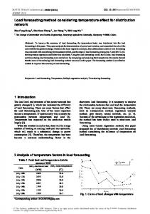
3. The Improved Exponential Smoothing Grey Model Because the traditional grey GM(1, 1) prediction model is only applicable to the case in which the data change is relatively gentle, it can neither meet the actual forecasting requirements without an ideal prediction effect nor consider the effects of influencing factors on it for the case where the data sequence has a fast growth rate or large fluctuation. Aimed at the disadvantage of the GM(1, 1) model (i.e., it cannot be applied to power load forecasting with fluctuation, complex environment, and obvious effects of influencing factors), an improved exponential smoothing grey prediction model is established in this paper using the selected main influencing factor variable and power load variable based on the analysis of short-term power load characteristics combining the grey correlation analysis, the exponential smoothing method, and the 0.618 method. By combining the influences of the main factors, the prediction model can expand the application scope of the grey prediction model, shorten the search interval when searching for the optimal smooth coefficient using the 0.618 method, and further improve the prediction accuracy and reliability. As shown in Figure 2, the concrete processes of the improved exponential smoothing grey model are as follows. Step 1. Input the real-time data of the original power load and perform the grey correlation analysis to determine the main influencing factor of the predicted object.
Step 2. Perform the first exponential smoothing processing to weaken its stochastic volatility and make it closer to the exponential trend. Step 3. Make predictions for the smoothed sequence using the grey model with an optimized background value. Step 4. The predicted results are restored to the predicted values of the original power load data and the data at the next prediction time through the inverse exponential smoothing processing. Step 5. Judge whether the predicted results reach the requirement of the fitting error. If they do, then output the predicted results. If they do not, then the 0.618 method is introduced, which reselects the subinterval of smoothing coefficient and the pilot smoothing coefficient and then judges the pilot smoothing coefficient. If it reaches |𝛼𝑖 − 𝛼𝑖 | < 𝜀, where 𝛼𝑖 and 𝛼𝑖 are the first pilot smoothing coefficient and the second pilot smoothing coefficient in the 𝑖th subinterval, respectively, and 𝜀 is the accuracy requirement, then take the optimal smooth coefficient 𝛼𝑖∗ = (𝛼𝑖 + 𝛼𝑖 )/2 and continue the algorithm. If it does not, then take the 𝛼 value with a smaller MAPE (Mean Absolute Percentage Error) value and continue the algorithm. The key step in the above forecasting process is to dynamically update the original power load data. The total amount of the original power load data in the update process keeps unchanged, that is, selecting a suitable moving span. When moving a span every time, it removes the “oldest” data and adds the “latest” data so that each forecasting process
4
Mathematical Problems in Engineering
Start
Input the original power load data updated in real time
Grey correlation analysis
Single exponential smoothing processing Optimal smooth coefficient i∗ = (i + i )/2 Grey prediction model with optimized background value
Yes
|i − i| <
Inverse exponential smoothing processing
The requirement of the fitting error reached?
Choose the value with smaller MAPE
No
Reselect the subinterval of No
smoothing coefficient and the pilot
Yes Output the predicted data
End
Figure 2: The flow diagram of the improved exponential smoothing grey model.
corresponds to a particular optimal smoothing coefficient, which can implement the real-time correction of the prediction model parameter when the memory occupation stays the same. In addition, the smoothing processing of the original data sequence is similar to that in [30], which can not only display the data more smoothly, but also eliminate the random errors to a certain degree.
3.1. The Grey Correlation Analysis. The grey correlation analysis is a multivariable statistical analysis method, whose basic idea is to judge whether there is a correlation between any two factor variables according to the similarity degree of the curves’ geometrical shapes of various factor sequences. The closer the curve is, the closer the correlation between the corresponding sequences of variables is, that is, the greater
Mathematical Problems in Engineering
5
the correlation degree is, and vice versa [31]. The specific steps are as follows: (1) Determine the main behavior factor variable of the system x1 (the predicted object) and the influencing factor variable sequences x𝑖 : x1 = (𝑥11 , 𝑥12 , . . . , 𝑥1𝑘 ) , x𝑖 = (𝑥𝑖1 , 𝑥𝑖2 , . . . , 𝑥𝑖𝑘 ) , x1 .
(𝑖 = 2, 3, . . . , 𝑛) .
(3)
In the expression above, 𝑘 represents the data length of (2) Normalize each variable sequence and get the initial values x𝑖 as follows: x𝑖 =
x𝑖 = (𝑥𝑖1 , 𝑥𝑖2 , . . . , 𝑥𝑖𝑘 ), 𝑥𝑖1
(𝑖 = 1, 2, . . . , 𝑛) .
(4)
(3) Calculate the correlation coefficient between the main behavior sequence and each influencing factor sequence. Let Δ 𝑖𝑗 = |𝑥1𝑗 − 𝑥𝑖𝑗 |(𝑗 = 1, 2, . . . , 𝑘), where 𝑥𝑖𝑗 represents the 𝑗th initial value of the 𝑖th variable. The difference sequences can be expressed as the following sequence: Δi = (Δ 𝑖1 , Δ 𝑖2 , . . . , Δ 𝑖𝑘 ) (𝑖 = 2, 3, . . . , 𝑛). The maximum difference 𝑀 and the minimum difference 𝑚 can be calculated by the equations 𝑀 = max𝑖 {max𝑗 {Δ 𝑖𝑗 }} and 𝑚 = min𝑖 {min𝑗 {Δ 𝑖𝑗 }}. Therefore, the correlation coefficient can be calculated by the equation 𝜉𝑖𝑗 = (𝑚 + 𝜌𝑀)/(Δ 𝑖𝑗 + 𝜌𝑀). In the equation, the parameter 𝜌 ∈ (0, 1) and it is generally equal to 0.5 [32].
(4) Calculate the correlation degree. Based on the correlation coefficients above, one can get the correlation degree 𝛾𝑖 = (1/𝑘) ∑𝑘𝑗=1 𝜉𝑖𝑗 , (𝑖 = 2, 3, . . . , 𝑛), where 𝛾 > 0. And then one can select the main influencing factor and eliminate the secondary factors according to the correlation degree. By performing the grey correlation analysis for each influencing factor and the main behavior variable, the result can provide the basis for the selection of the variables in the prediction model and avoid that the unrelated factors or the factors with small correlation degree affect the prediction efficiency of the whole system and reduce the prediction accuracy. 3.2. The Improvements of the Traditional Grey Prediction Model. The traditional grey prediction model requires that the predicted load sequence should conform with the exponential trend. The improvement of smoothness of the load sequence helps to improve the prediction accuracy of the grey model. Therefore, the improvements of the traditional grey prediction model lie mainly in two aspects: (1) the transformation of the original sequence, that is, to improve its smoothness, which makes it closer to the exponential law, and (2) the optimization of model parameters, that is, to optimize and transform the background value used for solving the grey
parameters. The original power load data is amended using the first exponential smoothing method of the exponential smoothing method in the improved grey prediction model, which weakens its stochastic volatility and makes the original data sequence more smoothly close to the exponential law. It also implements the prediction restoration of the original power load data and the data at the next prediction time using the inverse exponential smoothing in the final processing. As shown in Figure 3, the improved grey prediction model includes the following steps. (1) Firstly, perform the grey correlation analysis for the input original data sequence 𝑥𝑖0 . And then perform the first exponential smoothing processing for the selected variables using (5) to improve the smoothness of the sequence and make it meet the requirement of the input data in the grey prediction model. The smooth coefficient in the first exponential smoothing equation is obtained by the optimization of the 0.618 method. Finally, perform the accumulated generation for the obtained smoothed sequence 𝑆𝑖0 . As shown in (6), we can obtain the accumulative sequence 𝑦𝑖1 , where the superscript 0 represents the sequence that did not undergo accumulated generation and the superscript 1 represents the sequence that underwent accumulated generation. Moreover, 𝑖 = 1, 2, . . . , 𝑛, 𝑘 = 2, 3, . . . , 𝑞, where 𝑛 represents the number of variables selected by the grey correlation analysis and 𝑞 represents the number of the original power load data: 𝑆𝑖0 (𝑘) = 𝛼∗ 𝑥𝑖0 (𝑘) + (1 − 𝛼∗ ) 𝑆𝑖0 (𝑘 − 1) ,
(5)
𝑦𝑖1 (𝑘) = 𝑆𝑖0 (𝑘) + 𝑆𝑖0 (𝑘 + 1) .
(6)
(2) Optimize the background value 𝑍𝑖 in the grey prediction model according to (7) using the optimal smooth coefficient 𝛼∗ used in the first exponential smoothing processing. Calculate the data matrices 𝐿 and 𝑅 according to the optimized background value as shown in (8) and finally obtain the grey parameters 𝐶 and 𝐷 whose equations are as follows. The weight 𝛽 of the background value 𝑍𝑖 in the grey prediction model is taken as the value related to the optimal smooth coefficient 𝛼∗ , which can avoid the error caused by fixing 𝛽 to 0.5 in the traditional grey prediction model and help to improve the prediction precision: 𝛽=
1 1 − ∗ , 𝛼∗ 𝑒𝛼 − 1
𝑍𝑖 (𝑘) = 𝛽𝑦𝑖1 (𝑘 − 1) + (1 − 𝛽) 𝑦𝑖1 (𝑘) .
(7) (8)
In (8), the superscript 1 represents the notion that the sequence has been accumulated. And 𝑖 = 1, 2, . . . , 𝑛, 𝑘 = 2, 3, . . . , 𝑞, where 𝑛 represents the number of variables selected by the grey correlation analysis and 𝑞 represents the number of the original power load data: 𝑍1 (2) 𝑍2 (2) ⋅ ⋅ ⋅ 𝑍𝑛 (2) 1 [ 𝑍 (3) 𝑍 (3) ⋅ ⋅ ⋅ 𝑍 (3) 1 ] [ 1 ] 2 𝑛 [ ] 𝐿=[ . , .. .. .. .. ] [ . ] . . . . ] [ . [ 𝑍1 (𝑞) 𝑍2 (𝑞) ⋅ ⋅ ⋅ 𝑍𝑛 (𝑞) 1 ]
(9)
6
Mathematical Problems in Engineering
Start
Input the original data sequence xi0 and perform the grey correlation analysis
Find the optimal smooth coefficient ∗ using the
Perform the first exponential smoothing processing Si0 (k) = ∗ xi0 (k) + (1 − ∗ )Si0 (k − 1)
0.618 method
Perform the accumulated generation yi1 (k) = Si0 (k) + Si0 (k − 1)
Optimize the background value ∗
∗
= 1/ − 1/(e − 1) Zi (k) = yi1 (k − 1) + (1 − )yi1 (k)
Calculate the data matrices L and R and the grey parameters C and D
Obtain the fitted value and the predicted value ypi1 of the sequence yi1 and obtain the fitted value and the predicted value Spi0 of the sequence Si0 by the inverse accumulated generation
Obtain the fitted value and the predicted value yi0 of the sequence xi0 by inverse exponential smoothing
End
Figure 3: The structure diagram of the improved grey prediction model. 0 𝑆0 (2) 𝑆20 (2) ⋅ ⋅ ⋅ 𝑆𝑛 (2) ] [ 1 0 ] [ 0 [ 𝑆1 (3) 𝑆20 (3) ⋅ ⋅ ⋅ 𝑆𝑛 (3) ] ] [ , 𝑅=[ . .. .. .. ] ] [ . . . [ . . ] ] [ 𝑆10 (𝑞) 𝑆20 (𝑞) ⋅ ⋅ ⋅ 𝑆0 (𝑞) ] [ 𝑛
𝐶𝑇 −1 [ 𝑇 ] = 𝐻 = (𝐿𝑇 𝐿) 𝐿𝑇 𝑅. 𝐷
(10)
(11)
In (11), 𝐻 is a matrix with an order of (𝑛 + 1) × 𝑛. 𝐶𝑇 takes the first 𝑛 rows of the 𝐻 matrix and 𝐷𝑇 takes the last row of the 𝐻 matrix. To, respectively, transpose the two submatrices, one can get the grey parameters 𝐶 and 𝐷, where 𝐶 is a matrix with the order of 𝑛 × 𝑛 and 𝐷 is a matrix with the order of 𝑛 × 1. (3) Obtain the predicted sequence 𝑦𝑝1𝑖 of the sequence 1 𝑦𝑖 according to the grey prediction (see (12)) and obtain the predicted sequence 𝑆𝑝0𝑖 of the sequence 𝑆𝑖0 by the inverse accumulated generation (see (13)).
Mathematical Problems in Engineering
7
𝑦𝑝𝑖1 (𝑘) = 𝑒𝐶(𝑘−1) (𝑦𝑖1 (1) + 𝐶−1 𝐷) − 𝐶−1 𝐷,
(12)
𝑆𝑝𝑖0 (𝑘) = 𝑦𝑝𝑖1 (𝑘) − 𝑦𝑝𝑖1 (𝑘 − 1) .
(13)
(4) Put the predicted sequence 𝑆𝑝0𝑖 obtained by the grey prediction equation into the inverse exponential smoothing model as shown in (14) to realize the prediction restoration of the original power load data and the data at the next prediction time, and finally obtain the predicted sequence 𝑦𝑖0 of the original power load data 𝑥𝑖0 and the data at the next prediction time: 𝑦𝑖0 (𝑘) =
(𝑆𝑝𝑖0 (𝑘) − (1 − 𝛼∗ ) 𝑆𝑝𝑖0 (𝑘 − 1)) 𝛼∗
.
(14)
3.3. The Improvement of the 0.618 Method. It can be seen from Figure 3 that the accuracy of the smooth coefficient is directly related to the prediction accuracy. Generally speaking, the MSE (Mean Square Error) or the MAD (Mean Absolute Deviation) will be chosen as the objective function in the 0.618 method to search for the optimal smooth coefficient. The value of MSE can be expressed as 𝑓MSE and its calculation formula is shown in (15). The value of MAD can be expressed as 𝑓MAD and its calculation formula is shown in (16). However, through the actual calculation, one can observe that choosing MAPE as the objective function can yield better effects. The value of MAPE can be expressed as 𝑓MAPE and its calculation formula is shown in (17). 𝑞
𝑓MSE = 𝑓MAD =
∑𝑖=1 (𝑥𝑖0 − 𝑦𝑖0 ) 𝑞 𝑞 ∑𝑖=1 𝑥𝑖0 − 𝑦𝑖0 𝑞
2
,
,
0 0 100 𝑥𝑖 − 𝑦𝑖 . = ∑ 𝑞 𝑖=1 𝑥𝑖0
(15)
(16)
𝑞
𝑓MAPE
(17)
In the equations, 𝑞 is the number of the original power load data. 𝑦𝑖0 is the predicted sequence of 𝑥𝑖0 , which is related to the smooth coefficient. One can see that 𝑓MAPE actually is a function of smooth coefficient. One can observe from (15) that MSE is the average of the sums of squares of the errors between the actual value and the predicted value, which makes MSE unable to measure the unbiasedness. Similarly, one can observe from (16) that MAD is the average of the sums of the absolute deviation between the actual value and the predicted value, but MAD fails to reflect the effect of the deviation on the actual value. Therefore, compared with MSE and MAD, it can not only more accurately reflect the deviation between the predicted value and the actual value, but also effectively measure the unbiasedness and improve the reliability of prediction using MAPE as the objective function of the 0.618 method. The specific processes of the improved 0.618 method can be divided into five steps, as shown in Figure 4. (1) Let 𝜀 = 0.01 and divide the smooth coefficient 𝛼 ∈ (0, 1) into 10 equidistant subintervals: 𝛼1 ∈ (0, 0.1), 𝛼2 ∈
(0.1, 0.2), . . . , 𝛼10 ∈ (0.9, 1). Select a subinterval 𝛼𝑖 ∈ (𝑎0 , 𝑏0 ) (𝑖 = 1, 2, . . . , 10), where 𝑎0 and 𝑏0 represent the left and right endpoints of the 𝑖th subinterval, respectively; proceed to the next step. Furthermore, the smooth coefficient interval is divided into 10 equidistant subintervals for meeting the requirement that the objective function of the 0.618 method is a unimodal function. Because it is difficult to prove that MAPE is a unimodal function in the whole interval of [0, 1], it is possible to distribute the extreme points of MAPE in different subintervals by dividing the interval equally so that MAPE is a unimodal function in each subinterval. Even though MAPE is not a unimodal function in each subinterval, there is a little impact on searching for the optimal value. The reason is that the function value at every point in each subinterval is close to its minimum and it is sufficient to meet the precision requirement of 𝜀 = 0.01 when the interval length is small to a certain extent (equal to 0.1 here). The basic idea of the 0.618 method can be found in [33]. (2) Take the first trial point and let the first pilot smoothing coefficient 𝛼𝑖 = 0.618𝑎0 + 0.382𝑏0 . (3) Take the second trial point and let the second pilot smoothing coefficient 𝛼𝑖 = 0.382𝑎0 + 0.618𝑏0 . (4) Judge whether |𝛼𝑖 − 𝛼𝑖 | < 𝜀 holds or not. If it holds, then take the optimal smooth coefficient 𝛼𝑖∗ = (𝛼𝑖 + 𝛼𝑖 )/2 and proceed to the subsequent process. If it does not, then proceed to step (5). (5) Calculate the MAPE values 𝑓1 (𝛼𝑖 ) and 𝑓2 (𝛼𝑖 ) corresponding to the two trial points and compare their values. If 𝑓1 (𝛼𝑖 ) < 𝑓2 (𝛼𝑖 ), 𝑎0 keeps constant, 𝑏0 = 𝛼𝑖 , 𝛼𝑖 = 𝛼𝑖 , and 𝑓2 (𝛼𝑖 ) = 𝑓1 (𝛼𝑖 ), and proceed to step (2). If 𝑓1 (𝛼𝑖 ) > 𝑓2 (𝛼𝑖 ), 𝑏0 keeps constant, 𝑎0 = 𝛼𝑖 , 𝛼𝑖 = 𝛼𝑖 , and 𝑓1 (𝛼𝑖 ) = 𝑓2 (𝛼𝑖 ), and proceed to step (3).
4. Simulated Results and Discussion As shown in Table 1, the electricity consumption of the whole society and the national economic indicators, that is, the influencing factors data in 8 time periods of Fujian Province in [32], are adopted. The factors affecting the electricity consumption 𝑥1 in the table include the GDP (Gross Domestic Product) 𝑥2 , the total population 𝑥3 , and the import and export total 𝑥4 . In order to verify the validity of the proposed improved prediction algorithm, this paper realized the power load forecasting algorithm based on the improved exponential smoothing grey model, which builds the model using the electricity consumption data and its influencing factors data in 8 time periods shown in Table 1 and predicts the electricity consumption data in the next 2 time periods. (1) Determine the main factor variable affecting the power load forecasting using the grey correlation analysis. One can calculate the correlation degree of 3 influencing factors in Table 1 for the power load, and the results are shown in Table 2. One can observe from the calculation results of the correlation degree in Table 2 that the correlation degree between the import and export total and the electricity consumption is the largest one; that is, the influencing factor
8
Mathematical Problems in Engineering
Start
Let = 0.01, divide ∈ (0, 1) into 10 equidistant subintervals, and let i ∈ (a0 , b0 )
Let b0 = i , i = i f2 (i )
Solve the first pilot and let i = 0.618a 0 + 0.382b0
= f1 (i )
Let a 0 = i , i = i
Solve the second pilot and let i = 0.382a0 + 0.618b0
f1 (i ) = f2 (i ) No
Yes
No
f1 (i ) < f2 (i )
|i − i| <
Yes Respectively, calculate the MAPE values f1 (i ) ;H> f2 (i )
Take the optimal smooth coefficient i∗ = (i + i )/2
Put it into the first exponential smoothing equation
End
Figure 4: The structure diagram of the improved 0.618 method. Table 1: The original electricity consumption and its influencing factors data. Time/𝑡 1 2 3 4 5 6 7 8
𝑥1 (GWh) 18701.75 22364.49 25947.70 27994.90 29973.13 32019.54 35337.03 40151.49
𝑥2 (billion $) 18.805 27.928 35.765 42.668 49.575 54.776 59.171 65.335
“the import and export total” has the greatest influence on the electricity consumption. Therefore, the import and export total is chosen as the main influencing factor variable. (2) Build the improved exponential smoothing grey model and make predictions. After determining the main factor variable according to Table 2, one can build the multivariable grey model of the electricity consumption and the import and export total using
𝑥3 (million $) 31.50 31.83 32.37 32.61 32.82 32.99 33.16 34.10
𝑥4 (million $) 10041.81 12189.53 14445.69 15519.72 17952.80 17160.65 17619.56 21223.32
the original data in Table 1. The grey parameters can be obtained by (11). Subsequently, the corresponding differential equations are solved. The data in the first 8 time periods are used to fit the model and the fitted results are shown in Table 3. The fitted errors in Table 3 are calculated by (17), such as (|22364.49 − 23037.539|/22364.49) × 100% = 3.01%. The data in the last 2 time periods are used to verify the performance of the prediction model and the
Mathematical Problems in Engineering
9
Table 2: The correlation degree between each influencing factor and electricity consumption. Influencing factors Correlation degree
GDP/𝑥2 0.5185
Total population/𝑥3 0.6110
Import and export total/𝑥4 0.9243
Table 3: Comparison of the actual values and the fitted values of electricity consumption. Time/𝑡 1 2 3 4 5 6 7 8
Original data 18701.75 22364.49 25947.70 27994.90 29973.13 32019.54 35337.03 40151.49
The improved model Fitted data Error/% 18701.75 0 23037.539 3.01 24884.68 4.1 26963.009 3.69 29326.489 2.16 32046.51 0.08 35218.013 0.34 38967.811 2.95
The model in [32] Fitted data Error/% 18701.75 0 22891.98 2.36 24724.49 4.71 26747.38 4.46 28999.09 3.25 31531.90 1.52 34418.07 2.60 41695.84 3.85
Table 4: Comparison of the actual values and the predicted values of electricity consumption. Time Original values 9 10
43918.60 49682.87 Average error %
The improved model GM(1, 1) model GM(1, 4) model The model in [32] Predicted values Error/% Predicted values Error/% Predicted values Error/% Predicted values Error/% 43465.89 1.03 43017.38 2.05 42963.27 2.18 43465.89 1.03 48940.73 1.49 47065.22 5.27 48044.23 3.30 48907.30 1.56 1.26 3.66 2.74 1.30
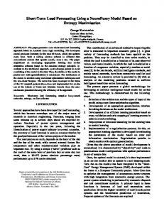
predicted results are shown in Table 4. The predicted errors in Table 4 are calculated by (17), such as (|43918.60 − 43465.89|/43918.60) × 100% = 1.03%. It can be seen from Table 3 that the fitted effect obtained by the improved prediction model is better than that in [32]. The parameters of the improved prediction model can be modified and optimized in real time according to the trend of the actual data. However, because the parameters of the model in [32] are fixed and the original data is not processed by any smoothing operations, the trend of the fitted data will be somewhat deviated from the trend of the actual data. It can be seen from Table 4 that the predicted effect obtained by the improved prediction model is the best and its predicted average MAPE value is 1.26% which meets the requirement that the average error in short-term power load forecasting should be around 3%. Although the error of the improved prediction model is only slightly smaller than that in [32], the electricity consumption difference will be large when used in an actual application, for example, 50000 × 0.0126 = 630 (GWh), 50000 × 0.013 = 650 (GWh), and the electricity consumption difference EC𝑑 = 20 (GWh). If such a large electricity consumption difference is taken into account, it will save a very large economic cost. Especially for the large industrial consumers with a large electricity consumption base, it will be conducive to selecting a more reasonable charging mode by accurately forecasting the power demand for the next month, which makes the economic effect more obvious. This phenomenon also illustrates three problems: (1) if the influencing factors were not taken into consideration in the prediction model, it
would lead to a poor prediction accuracy, such as the GM(1, 1) model; (2) if other secondary influencing factors besides the main influencing factor were taken into consideration in the prediction model, the prediction error would also increase, such as the GM(1, 4) model; (3) if the influencing factors were considered in the prediction model but the model parameters were not optimized, it would also lead to an increase in prediction error, such as the model adopted in [32]. In order to show the degree of deviation between the actual value and the predicted value more intuitively, the curves of the actual value and the predicted value are plotted in Figure 5. It can be seen from Figure 5 that the trend of predicted values of power load is very close to the trend of actual value and the overall predicted effect is satisfactory. The simulated results show that the improved exponential smoothing grey prediction model is feasible and effective for short-term power load forecasting, which improves the prediction accuracy of the prediction model. Moreover, the introduction of the 0.618 method improves the solution efficiency and the automation and makes the predicted results highly reliable, which basically overcomes the shortcomings of the traditional grey prediction algorithm. Besides, the algorithm is straightforward to be realized.
5. Conclusion The traditional grey prediction model has found wide applications in the field of power load forecasting because of its characteristics of simple principle, lower sample data
10
Mathematical Problems in Engineering
5
×104
Conflicts of Interest The authors declare that there are no conflicts of interest regarding the publication of this paper.
Power load (GWh)
4.5 4
Acknowledgments
3.5
This work is partially supported by the 111 Project B14042 and the National Natural Science Foundation of China under Grants nos. 51490660 and 51405362.
3 2.5
References
2 1.5
1
2
3
4
5 6 7 Time (month)
8
9
10
Original values Predicted values
Figure 5: Comparison curves of the original values and the predicted values.
requirement, and ability to tackle uncertain problems. However, the disadvantages of the model itself result in its defective prediction effect and thus inability to meet the actual forecasting requirement. Aiming at the shortcomings of the above prediction model, this paper proposed a shortterm power load forecasting method based on the improved exponential smoothing grey model which not only preserves the advantages of the traditional grey prediction model for dealing with the poor information, but also analyzes the various influencing factors affecting power load forecasting using the grey correlation analysis and determines the main influencing factor. The improved prediction model reduces the calculation quantity and improves the prediction efficiency because it does not consider too much the secondary factors which can reduce the prediction efficiency. Some conclusions can be drawn as follows: (1) The first exponential smoothing model is employed to deal with the original power load data in the improved prediction model, which not only weakens the randomness but also improves the smoothness of data. The smoothing processing makes it close to the exponential trend, which meets the requirement of the input data in the grey prediction model and contributes to further improving the prediction accuracy. (2) The 0.618 method is introduced in the first exponential smoothing process and MAPE is chosen as the objective function to search for the optimal smooth coefficient, which enhances the reliability of prediction. (3) The background value of the traditional grey prediction model is also optimized, which can implement the real-time correction of the prediction model parameter.
[1] Y. He, Q. Xu, J. Wan, and S. Yang, “Short-term power load probability density forecasting based on quantile regression neural network and triangle kernel function,” Energy, vol. 114, pp. 498–512, 2016. [2] Z. Zhang and W. Gong, “Short-term load forecasting model based on quantum elman neural networks,” Mathematical Problems in Engineering, vol. 2016, Article ID 7910971, 2016. [3] X. Wang and Y. Wang, “A Hybrid Model of EMD and PSOSVR for Short-Term Load Forecasting in Residential Quarters,” Mathematical Problems in Engineering, vol. 2016, Article ID 9895639, 2016. [4] R. Hu, S. Wen, Z. Zeng, and T. Huang, “A short-term power load forecasting model based on the generalized regression neural network with decreasing step fruit fly optimization algorithm,” Neurocomputing, vol. 221, pp. 24–31, 2017. [5] H. Li, L. Cui, and S. Guo, “A hybrid short-term power load forecasting model based on the singular spectrum analysis and autoregressive model,” Advances in Electrical Engineering, vol. 2014, Article ID 424781, 7 pages, 2014. [6] H. Yuansheng, H. Shenhai, and S. Jiayin, “A novel hybrid method for short-term power load forecasting,” Journal of Electrical and Computer Engineering, vol. 2016, Article ID 2165324, 2016. [7] Y. He, R. Liu, H. Li, S. Wang, and X. Lu, “Short-term power load probability density forecasting method using kernel-based support vector quantile regression and Copula theory,” Applied Energy, vol. 185, pp. 254–266, 2017. [8] M. Capuno, J.-S. Kim, and H. Song, “Very short-term load forecasting using hybrid algebraic prediction and support vector regression,” Mathematical Problems in Engineering, vol. 2017, Article ID 8298531, 2017. [9] H. J. Sadaei, F. G. Guimaraes, C. Silva, M. H. Lee, and T. Eslami, “Short-term load forecasting method based on fuzzy time series, seasonality and long memory process,” International Journal of Approximate Reasoning, vol. 83, pp. 196–217, 2017. [10] A. Laouafi, M. Mordjaoui, S. Haddad, T. E. Boukelia, and A. Ganouche, “Online electricity demand forecasting based on an effective forecast combination methodology,” Electric Power Systems Research, vol. 148, pp. 35–47, 2017. [11] Y. Chen, P. Xu, Y. Chu et al., “Short-term electrical load forecasting using the Support Vector Regression (SVR) model to calculate the demand response baseline for office buildings,” Applied Energy, vol. 195, pp. 659–670, 2017. [12] B. Wang, D. Wang, and S. Zhang, “Short-term Distributed Power Load Forecasting Algorithm Based on Spark and IPPSO LSSVM,” Electric Power Automation Equipment, vol. 36, no. 1, pp. 117–122, 2016.
Mathematical Problems in Engineering [13] S. Brodowski, A. Bielecki, and M. Filocha, “A hybrid system for forecasting 24-h power load profile for Polish electric grid,” Applied Soft Computing, vol. 58, pp. 527–539, 2017. [14] M. B. Germi, M. Mirjavadi, A. S. S. Namin, and A. Baziar, “A hybrid model for daily peak load power forecasting based on SAMBA and neural network,” Journal of Intelligent & Fuzzy Systems: Applications in Engineering and Technology, vol. 27, no. 2, pp. 913–920, 2014. [15] L. Xiao, W. Shao, C. Wang, K. Zhang, and H. Lu, “Research and application of a hybrid model based on multi-objective optimization for electrical load forecasting,” Applied Energy, vol. 180, pp. 213–233, 2016. [16] S. Zhang, R. Shi, L. Zhang, B. Yan, H. Zhang, and P. He, “Improvement of chaotic forecasting model and its application in power daily load forecasting,” Chinese Journal of Scientific Instrument, vol. 37, no. 1, pp. 208–214, 2016. [17] L. Xiao, W. Shao, T. Liang, and C. Wang, “A combined model based on multiple seasonal patterns and modified firefly algorithm for electrical load forecasting,” Applied Energy, vol. 167, pp. 135–153, 2016. [18] K. G. Boroojeni, M. H. Amini, S. Bahrami, S. S. Iyengar, A. I. Sarwat, and O. Karabasoglu, “A novel multi-time-scale modeling for electric power demand forecasting: From short-term to medium-term horizon,” Electric Power Systems Research, vol. 142, pp. 58–73, 2017. [19] N. Xie and S. Liu, “Interval grey number sequence prediction by using non-homogenous exponential discrete grey forecasting model,” Journal of Systems Engineering and Electronics, vol. 26, no. 1, pp. 96–102, 2015. [20] N. Xu, Y. Dang, and Y. Gong, “Novel grey prediction model with nonlinear optimized time response method for forecasting of electricity consumption in China,” Energy, vol. 118, pp. 473–480, 2017. [21] L. Jian-Kai, C. Cattani, and S. Wan-Qing, “Power load prediction based on fractal theory,” Advances in Mathematical Physics, vol. 2015, Article ID 827238, 2015. [22] B. Zeng and C. Li, “Forecasting the natural gas demand in China using a self-adapting intelligent grey model,” Energy, vol. 112, pp. 810–825, 2016. [23] S. Liu and L.-X. Tian, “The study of long-term electricity load forecasting based on improved grey prediction model,” in Proceedings of the 12th International Conference on Machine Learning and Cybernetics, ICMLC 2013, pp. 653–657, China, July 2013. [24] J. Massana, C. Pous, L. Burgas, J. Melendez, and J. Colomer, “Short-term load forecasting for non-residential buildings contrasting artificial occupancy attributes,” Energy and Buildings, vol. 130, pp. 519–531, 2016. [25] H. Zhao and S. Guo, “An optimized grey model for annual power load forecasting,” Energy, vol. 107, pp. 272–286, 2016. [26] M. Y. Tong, X. H. Zhou, and B. Zeng, “The background value optimization method in grey NGM (1,1, k) model,” Control and Decision, vol. 32, no. 3, 2017. [27] P. Ji, D. Xiong, P. Wang, and J. Chen, “A study on exponential smoothing model for load forecasting,” in Proceedings of the 2012 Asia-Pacific Power and Energy Engineering Conference, APPEEC 2012, China, March 2012. [28] J. A. Koupaei, S. Hosseini, and F. M. Ghaini, “A new optimization algorithm based on chaotic maps and golden section search method,” Engineering Applications of Artificial Intelligence, vol. 50, pp. 201–214, 2016.
11 [29] Y. Yang and D. Xue, “Continuous fractional-order grey model and electricity prediction research based on the observation error feedback,” Energy, vol. 115, pp. 722–733, 2016. [30] E. Cadenas, O. A. Jaramillo, and W. Rivera, “Analysis and forecasting of wind velocity in chetumal, quintana roo, using the single exponential smoothing method,” Journal of Renewable Energy, vol. 35, no. 5, pp. 925–930, 2010. [31] X. Xia, Y. Sun, K. Wu, and Q. Jiang, “Optimization of a straw ring-die briquetting process combined analytic hierarchy process and grey correlation analysis method,” Fuel Processing Technology, vol. 152, pp. 303–309, 2016. [32] Y. P. Wang, D. X. Huang, H. Q. Xiong, and Y. L. Niu, “Using relational analysis and multi-variable grey model for electricity demand forecasting in smart grid environment,” Power System Protection and Control, vol. 40, no. 1, pp. 96–100, 2012. [33] Y. X. Yuan and W. Y. Sun, Optimization theory and method, Science Press, Beijing, China, 1997, 96–99.
Advances in
Operations Research Hindawi Publishing Corporation http://www.hindawi.com
Volume 2014
Advances in
Decision Sciences Hindawi Publishing Corporation http://www.hindawi.com
Volume 2014
Journal of
Applied Mathematics
Algebra
Hindawi Publishing Corporation http://www.hindawi.com
Hindawi Publishing Corporation http://www.hindawi.com
Volume 2014
Journal of
Probability and Statistics Volume 2014
The Scientific World Journal Hindawi Publishing Corporation http://www.hindawi.com
Hindawi Publishing Corporation http://www.hindawi.com
Volume 2014
International Journal of
Differential Equations Hindawi Publishing Corporation http://www.hindawi.com
Volume 2014
Volume 2014
Submit your manuscripts at https://www.hindawi.com International Journal of
Advances in
Combinatorics Hindawi Publishing Corporation http://www.hindawi.com
Mathematical Physics Hindawi Publishing Corporation http://www.hindawi.com
Volume 2014
Journal of
Complex Analysis Hindawi Publishing Corporation http://www.hindawi.com
Volume 2014
International Journal of Mathematics and Mathematical Sciences
Mathematical Problems in Engineering
Journal of
Mathematics Hindawi Publishing Corporation http://www.hindawi.com
Volume 2014
Hindawi Publishing Corporation http://www.hindawi.com
Volume 2014
Volume 2014
Hindawi Publishing Corporation http://www.hindawi.com
Volume 2014
Discrete Mathematics
Journal of
Volume 2014
Hindawi Publishing Corporation http://www.hindawi.com
Discrete Dynamics in Nature and Society
Journal of
Function Spaces Hindawi Publishing Corporation http://www.hindawi.com
Abstract and Applied Analysis
Volume 2014
Hindawi Publishing Corporation http://www.hindawi.com
Volume 2014
Hindawi Publishing Corporation http://www.hindawi.com
Volume 2014
International Journal of
Journal of
Stochastic Analysis
Optimization
Hindawi Publishing Corporation http://www.hindawi.com
Hindawi Publishing Corporation http://www.hindawi.com
Volume 2014
Volume 2014