Hindawi Advances in Meteorology Volume 2017, Article ID 6856139, 22 pages https://doi.org/10.1155/2017/6856139
Research Article Short-Term Wind Speed Prediction Using EEMD-LSSVM Model Aiqing Kang,1 Qingxiong Tan,2 Xiaohui Yuan,2 Xiaohui Lei,1 and Yanbin Yuan3 1
State Key Laboratory of Simulation and Regulation of Water Cycle in River Basin, China Institute of Water Resources and Hydropower Research, Beijing 100038, China 2 School of Hydropower and Information Engineering, Huazhong University of Science and Technology, Wuhan 430074, China 3 School of Resource and Environmental Engineering, Wuhan University of Technology, Wuhan 430070, China Correspondence should be addressed to Xiaohui Yuan;
[email protected] and Xiaohui Lei; leixiaohui
[email protected] Received 1 August 2017; Revised 6 November 2017; Accepted 14 November 2017; Published 12 December 2017 Academic Editor: Ilan Levy Copyright © 2017 Aiqing Kang et al. This is an open access article distributed under the Creative Commons Attribution License, which permits unrestricted use, distribution, and reproduction in any medium, provided the original work is properly cited. Hybrid Ensemble Empirical Mode Decomposition (EEMD) and Least Square Support Vector Machine (LSSVM) is proposed to improve short-term wind speed forecasting precision. The EEMD is firstly utilized to decompose the original wind speed time series into a set of subseries. Then the LSSVM models are established to forecast these subseries. Partial autocorrelation function is adopted to analyze the inner relationships between the historical wind speed series in order to determine input variables of LSSVM models for prediction of every subseries. Finally, the superposition principle is employed to sum the predicted values of every subseries as the final wind speed prediction. The performance of hybrid model is evaluated based on six metrics. Compared with LSSVM, Back Propagation Neural Networks (BP), Auto-Regressive Integrated Moving Average (ARIMA), combination of Empirical Mode Decomposition (EMD) with LSSVM, and hybrid EEMD with ARIMA models, the wind speed forecasting results show that the proposed hybrid model outperforms these models in terms of six metrics. Furthermore, the scatter diagrams of predicted versus actual wind speed and histograms of prediction errors are presented to verify the superiority of the hybrid model in short-term wind speed prediction.
1. Introduction With the rapid economic development and increasing environmental pollution, the renewable, clean, and pollutionfree wind energy is showing promising application prospect. In 2016, the totally installed world wind power capacity increased to 486.7 GW with the newly installed 54.8 GW. The corresponding global growth rate was 11.8%. Meanwhile the newly installed wind power capacity was 23.4 GW and the total capacity reached 168.7 GW with the growth rate of 14.0% for China [1]. To promote the quantity application of wind energy, electricity generated from wind power needs to be connected to the grid so as to be transferred to areas that consume lots of electric energy [2, 3]. Furthermore, during the process of wind energy being transformed into electricity, accurate control should be conducted so that higher generation efficiency can be obtained [4, 5]. However, the intermittency and randomness nature characteristics of wind speed caused great challenges to integration of wind
power and the control operation of wind turbines. Therefore, accurate short-term wind speed prediction model should be built to overcome these challenges [6, 7]. There are mainly three kinds of wind speed prediction methods, namely, the physical, the statistical, and hybrid approaches. The principle underlying the physical model is to find out the mapping relation among wind speed, temperature, pressure, and moisture and build the thermodynamics formulae from numerical weather prediction (NWP) models [8]. This kind of model is good at medium- and long-term wind speed prediction. However, the detection and collection of these information data needs a lot of sensors, which can be very expensive. Furthermore, solving this kind of model requires complex calculations. These disadvantages limit the application of the physical model. The statistical model is used more widely than the physical model at short-term and ultra-short-term wind speed prediction. The building process of statistical model is relatively simple, which focuses on seeking rules hidden in the wind data by studying the
2 historical wind speed time series and using these rules to forecast wind speed without considering meteorological conditions [9]. The basic idea of the hybrid approach is to combine different approaches (numerical weather models, statistical approaches, and machine learning algorithms), retaining advantages of each approach. Due to the fact that different prediction models can supplement the capturing properties of wind speed time series, hybrid method may perform much better than any individual forecasting model [8, 9]. In this paper, a hybrid model that combines Ensemble Empirical Mode Decomposition (EEMD) with Least Square Support Vector Machine (LSSVM) is proposed to forecast short-term wind speed accurately. The hybrid model makes use of the decomposition ability of the EEMD algorithm, as well as the forecasting superiority of the LSSVM model. The EEMD is firstly applied to decompose the original wind speed time series into a set of relative stable subseries involving only one mode. Then the partial autocorrelation function (PACF) is utilized to analyze the characteristics of each subseries so as to determine a suitable input of the LSSVM model for each subseries. Next, LSSVM model is employed to produce one-step-ahead and multi-step-ahead predictions for the corresponding subseries. Finally, the forecasting values of all the subseries are integrated as the final wind speed predictions. To validate the prediction performance of the proposed hybrid model (EEMD-LSSVM), LSSVM, Back Propagation (BP) Neural Networks, Auto-Regressive Integrated Moving Average (ARIMA), hybrid of EEMD with ARIMA, and hybrid Empirical Mode Decomposition (EMD) with LSSVM, they are used to produce one-step-ahead and multi-step-ahead predictions for 10-min intervals wind speed time series collected from a wind farm in Galicia, Spain. Furthermore, the scatter diagrams of predicted versus actual wind speed and histograms of prediction errors of different models are discussed in detail. They demonstrate that the short-term wind speed prediction obtained by the proposed hybrid model has a higher correlation with actual wind speed series. The forecasting results prove that the proposed hybrid model outperforms these compared models for short-term wind speed prediction. The remainder of this paper is organized as follows. Section 2 discusses the related work on short-term wind speed predictions. Section 3 overviews the Ensemble Empirical Mode Decomposition. Section 4 reviews the basic principle of least square support vector machine. Section 5 presents the hybrid EEMD-LSSVM model for prediction of wind speed. Section 6 gives experimental and comparison results of two cases. Section 7 summarizes the conclusions. Acknowledgments are listed at the end.
2. Related Work In this section, we review a few popular approaches for prediction of short-term wind speed. Time series models, such as autoregressive moving average (ARMA) [10] and ARIMA [11], are widely used for short-term wind speed prediction. In recent years, some improved time series models have been proposed for wind forecasting. Kavasseri
Advances in Meteorology and Seetharaman [12] apply the fractional-ARIMA model on wind speed forecasting on the day-ahead and two-dayahead horizons at four potential wind generation sites located in North Dakota, USA. The simulated results show that fractional-ARIMA outperforms ARIMA when wind speed series appear to have long-memory characteristics. Erdem and Shi [13] put forward four approaches based on ARMA for prediction of hourly wind speed, and satisfactory simulation results were obtained. Ambach and Schmid [14] built a time-varying regression model for short-term wind speed prediction, composed of Autoregressive Fractionally Integrated Moving Average (ARFIMA) and Asymmetric Power Generalized Autoregressive Conditional Heteroscedasticity (APARCH). The forecasting results prove that the ARFIMAAPARCH model has a higher prediction precision, as compared with Support Vector Regression (SVR). However, prediction performances of the time series model depend on the selection of model parameters. Furthermore, the time series model cannot capture the nonlinear component of the wind speed series, which limits the forecasting accuracy of the model. Salcedo-Sanz et al. [15] present the application of evolutionary-based approaches to optimize the hyperparameters in Support Vector Machines (SVM) and discuss the performance of evolutionary SVR algorithm for wind speed prediction in a wind farm located at the south of Spain. References [16, 17] study the performance of hourly ahead wind speed forecasting by LSSVM, in which the typical kernel function (linear, polynomial, and Gaussian kernels) and the related parameters on the forecasting accuracy are investigated. An adaptive robust methodology (Bayesian model averaging) has been developed to forecast hourly wind speed forecasting at two North Dakota sites [18]. This Bayesian model averaging methodology provides a unified approach to tackle the challenging model selection issue in wind speed forecasting. By incorporating domain knowledge about wind speed as a prior, Bayesian structural break model is proposed to forecast very short-term wind speed and it is tested with wind speed data collected from utility-scale wind turbines [19]. Cadenas and Rivera [20] make use of Artificial Neural Networks (ANN) to forecast the hourly wind speed series collected from observation points located in La Venta, Oaxaca, Mexico. The results show that this model has high prediction accuracy for short-term wind speed forecasting. Application of different ANN models (Adaptive Linear Element, BP, and radial basis function) in one-hour-ahead wind speed forecasting is investigated [21, 22]. The superiority of the ANN models is demonstrated and found to be successful and feasible. Flores et al. [23] make a comparison of wind speed prediction performance between the ARMA and ANN which are both optimized by Genetic Algorithms (GA). In their research, the results demonstrate that the performance of the ANN model outperforms the ARMA model. Hong et al. [24] propose a Multilayer Feed-forward Neural Network (MFNN) to predict wind speed at different time horizons. The MFNN model has a better performance as compared with the traditional forecasting models. Wu et al. [25] make use of the single multiplicative neuron model and the iterated nonlinear filters to build two models to forecast wind speed. The forecasting performance of hourly wind speed data collected
Advances in Meteorology from three stations shows that the proposed two models are better than ARMA, ANN, Kernel Ridge Regression, and single multiplicative neuron. Although both the time series model and the machine learning model can improve the prediction accuracy to some extent, after their parameters are optimized, the highly complex wind speed time series are still beyond their description capability. Due to the various inherent modes in wind speed series, the single model, such as ARIMA and ANN, can not completely capture the characteristics of wind speed data [26]. Therefore, the disadvantages limit the performance of two models for wind speed prediction. Recently, hybrid approaches have been focused on improving the wind speed prediction precision. Different hybrid wind speed prediction models have been proposed in the literature in order to benefit from the unique capability of single models [27–37]. Salcedo-Sanz et al. [27] proposes the hybridization of the fifth-generation mesoscale physical forecasting model (MM5) with neural networks for shortterm wind speed prediction of a wind park located at Albacete in Spain. This hybrid model integrates a global numerical weather prediction model and observations at different heights as initial and boundary conditions for the MM5 model. Subsequently, an ANN model is employed to forecast the wind speed by using the outputs of the MM5 model. The wind speed forecast obtained by the hybrid model is close to the measured value. Based on different global forecasting models and banks of regression SVM, OrtizGarc´ıa et al. [28] improve a wind speed prediction system on a wind farm in southeast Spain. Several SVM structures are adopted to manage the diversity in input data arising from different global forecasting models and several parameterizations of a mesoscale model. The system implementing SVM outperforms the similar system using multilayer perceptrons. Shukur and Lee [29] combine ARIMA, ANN, and Kalman filter (KF) as a new algorithm to forecast daily wind speed, and the proposed hybrid model outperforms ARIMA, ANN, and KF models. Guo et al. [30] propose a hybrid model composed of Seasonal Auto-Regression Integrated Moving Average (SARIMA) and LSSVM for forecasting monthly wind speed of two observation stations located at the Hexi Corridor in China. The simulation results show that the hybrid SARIMA and LSSVM model has a stronger forecasting ability, compared with ARIMA, LSSVM, SARIMA, and ARIMA-SVM. Liu et al. [31] discuss two hybrid models (ARIMA-ANN, ARIMA-Kalman) for prediction of hourly wind speed. The results of two cases show that the forecasting precisions of both hybrid ARIMA-ANN and ARIMAKalman models are higher than those of single models. Yu et al. [32] combine Gaussian Mixture Copula Model (GMCM) and Gaussian Process Regression (GPR) as a wind speed forecasting method. The results show that GMCM-GPR has a higher prediction accuracy than that of GMCM-ARIMA and GMCM-SVR. Bouzgou and Benoudjit [33] discuss a Multiple Architecture System (MAS) for wind speed prediction, which consists of Multiple Linear Regression (MLR), Multi-Layer Perceptrons (MLP), Radial Basis Functions (RBF), and SVM by different integration strategies. The MAS improves the forecasting precision to some extent, compared with the
3 traditional methods. Chen and Yu [34] integrate Unscented Kalman Filter (UKF) with SVM as an approach to predict wind speed collected from three observation stations located in Massachusetts, USA. The results show that the hybrid UKF-SVM model outperforms ANN, SVR, and Autoregressive Integrated with Kalman filter (AR-Kalman) in both onestep- and multi-step-ahead forecasting in terms of accuracy. However, the hybrid model suffers from the problem of selecting proper submodels. Furthermore, the distribution of suitable weight for each submodel is also a challenge. These defects limit the prediction performance of the hybrid model. The main procedure of other hybrid models is to utilize signal processing technology to decompose original wind speed time series into a set of subseries and then to build prediction models for each subseries. Liu et al. [35] combine Wavelet, Wavelet Packet, Time Series Analysis, and ANN to predict half-hourly wind speed data. In their study, the results prove that the hybrid models with the signal processing technology have better forecasting precision as compared with ARIMA and other traditional models. Guo et al. [36] combine Empirical Mode Decomposition (EMD) with Feed-Forward Neural Network (FNN) together as a hybrid model for forecasting monthly and daily wind speed. The results show that the modified EMD-FNN model has better performance for multi-step-ahead prediction as compared with traditional models. Hu et al. [37] compose Empirical Wavelet Transform (EWT), Coupled Simulated Annealing (CSA), and LSSVM as a hybrid model for short-term wind speed forecasting. Liu et al. [38] combine Extreme Learning Machines (ELM) with four signal decomposing algorithms for wind speed prediction. The forecasting results show that the hybrid models are better than single ELM models. It can be seen that the combination of signal processing technology and efficient forecasting model is a promising way to improve the wind speed prediction accuracy. The main data decomposition techniques are Wavelet Decomposition (WD) and EMD. WD has strong time-frequency analysis ability and hybrid model based WD has stronger prediction ability than the traditional models for wind speed prediction. However, WD is very sensitive to parameter selection. Some defects, such as the decomposition level selection, the option of the type, and order of mother Wavelet used in WD, have not been solved. These problems affect further application of WD for wind speed prediction. The EMD decomposes the data according to their own inherent time scale. Therefore, EMD algorithm avoids the process of setting base function. This essential difference enables EMD to overcome the defects of WD and shows strong processing capacity for nonstationary and nonlinear data set. However, further study reveals that EMD suffers from the mode mixing problem, which limits the decomposition effect [39]. Therefore, the EEMD algorithm is proposed, which overcomes the mode mixing problem by using an assistant procedure of adding white noise. As an efficient prediction algorithm, LSSVM overcomes the disadvantages of ANN, such as requirement of a large training set, getting trapped into local extrema, and overfitting.
4
Advances in Meteorology Decompose with EMD Input original time series y(t) Input signal yi (t), n = 1 Identify all the local extrema in yi (t)
Add white noise series ni (t)
Construct the upper envelope yi,OJ (t) and the lower envelope yi,FIQ (t) Obtain white noise-added time series yi (t)
yi (t) = ℎi (t)
mi (t) = (yi,OJ (t) + yi,FIQ (t))/2 ℎi (t) = yi (t) − mi (t)
yi (t) = ri,n (t)
No
If ℎi (t) is an IMF? Yes Obtain IMFs n = n + 1, ci,n (t) = ℎi (t), ri,n (t) = yi (t) − ci,n (t) Obtain ensemble means of corresponding IMFs
If ri,n (t) is a monotonic function?
No
Yes
The final IMFs decomposed by EEMD
Figure 1: The flowchart of EEMD algorithm.
3. Overview of Ensemble Empirical Mode Decomposition The EEMD algorithm was proposed by Wu and Huang in 2009 [40] so as to overcome EMD’s disadvantage of mode mixing problem, which means that one single intrinsic mode function (IMF) contains signals of different scales, or a signal of the same scale distributes in different IMFs. The basic idea of the EEMD is that the observed data integrates real time series and noise. Though the observed time series exhibit different noise level, the ensemble mean is close to the real time series. Based on this idea, the EEMD algorithm utilizes the assistance procedure of adding white noise. The noiseadded signal is then decomposed into a series of IMFs by using EMD. The influence of the added white noise can be counteracted with each other by using ensemble averaging. Therefore, the EEMD algorithm shows a more powerful processing capacity for complex and unstable time series data set as compared with EMD. The flowchart of the EEMD algorithm is given in Figure 1. The EEMD modeling process is given as follows.
Step 1. Add a white noise 𝑛𝑖 (𝑡) to the original time series 𝑦(𝑡). The noise-added signal 𝑦𝑖 (𝑡) is as follows: 𝑦𝑖 (𝑡) = 𝑦 (𝑡) + 𝑛𝑖 (𝑡) .
(1)
Step 2. Make use of the EMD algorithm to decompose 𝑦𝑖 (𝑡) into several IMF{𝑐𝑖,𝑗 (𝑡)} and a residual 𝑟𝑖 (𝑡), where {𝑐𝑖,𝑗 (𝑡)} is the 𝑗th IMF at the 𝑖th trial; 𝑟𝑖 (𝑡) is the residual at the 𝑖th trial. The implementation process of EMD is shown as follows: (1) Let 𝑟0 = 𝑦𝑖 (𝑡). (2) Find all the local maximums and minimums of 𝑦𝑖 (𝑡). (3) Construct the upper envelope 𝑦𝑖,up (𝑡) and the lower 𝑦𝑖,low (𝑡) through interpolating all the local maximums and minimums with cubic spline function. (4) Calculate the average value of the upper and lower envelopes. 𝑚𝑖 (𝑡) =
𝑦𝑖,up (𝑡) + 𝑦𝑖,low (𝑡) 2
.
(2)
Advances in Meteorology
5
(5) Extract the average value 𝑚𝑖 (𝑡) from the time series 𝑦𝑖 (𝑡), and define ℎ𝑖 (𝑡) as ℎ𝑖 (𝑡) = 𝑦𝑖 (𝑡) − 𝑚𝑖 (𝑡) .
(3)
(6) Check the properties of ℎ𝑖 (𝑡): if ℎ𝑖 (𝑡) satisfies the standard of stop criteria for screening IMF, the 𝑛th IMF is set as 𝑐𝑖,𝑛 (𝑡) = ℎ𝑖 (𝑡) and the residual error can be calculated with 𝑟𝑖,𝑛 (𝑡) = 𝑦𝑖 (𝑡) − 𝑐𝑖,𝑛 (𝑡). Otherwise, replace 𝑦𝑖 (𝑡) by ℎ𝑖 (𝑡). (7) If 𝑟𝑖,𝑛 (𝑡) satisfies the stop criteria of EMD, then 𝑟𝑖,𝑛 (𝑡) is the residual error. Otherwise, replace 𝑟𝑖,𝑛 (𝑡) by using 𝑦𝑖 (𝑡) and go back to step (2). After the sifting processing, the original time series 𝑦𝑖 (𝑡) can be described as the sum of all IMFs and a residual error: 𝑛
𝑦𝑖 (𝑡) = ∑ 𝑐𝑖,𝑗 (𝑡) + 𝑟𝑖,𝑛 (𝑡) , 𝑗=1
(4)
where 𝛾 is the adjustment parameter; 𝜉𝑖 is the error between the real value and estimated value of the 𝑖th sample. To solve this optimization problem, the following Lagrange function is constructed: 1 1 𝑛 𝐿 (𝜔, 𝑏, 𝜉, 𝛼) = 𝜔𝑇 𝜔 + 𝛾 ∑ 𝜉𝑖 2 2 2 𝑖=1 𝑛
− ∑ 𝛽𝑖 [𝜔𝑇 𝜑 (𝑥𝑖 ) + 𝑏 + 𝜉𝑖 − 𝑦𝑖 ] , 𝑖=1
where 𝛽𝑖 represents the Lagrange multiplier. According to the Karush-Kuhn-Tucker (KKT) conditions, the following expression can be obtained. 𝜕𝐿 = 0 → 𝜕𝜔
where 𝑛 is the number of IMF; 𝑐𝑖,𝑗 (𝑡) is the 𝑛th IMF when adding the 𝑖th noise; 𝑟𝑖,𝑛 (𝑡) is the final residual error when adding the 𝑖th noise.
𝑛
𝜔 = ∑ 𝛽𝑖 𝜑 (𝑥𝑖 ) 𝑖=1
Step 3. Repeat 𝑁 times for Steps 1 and 2 with different white noise 𝑛𝑖 (𝑡), 𝑖 = 1, 2, . . . , 𝑁.
𝜕𝐿 = 0 → 𝜕𝑏
Step 4. Calculate the ensemble mean 𝑐𝑗 (𝑡) of all the corresponding IMFs during 𝑁 times trials as the final result. The calculation formula is as follows: 𝑐𝑗 (𝑡) =
𝑁
∑ 𝛽𝑖 = 0 𝑖=1
𝑁
1 ∑ 𝑐 (𝑡) , 𝑁 𝑖=1 𝑖,𝑗
The LSSVM proposed by Suykens and Vandewalle in 2000 [41] is a modified version of SVM based on the least squares theory. The LSSVM replaces a complex quadratic programming problem with a set of relative simple linear equations compared with SVM. For a given training data set {(𝑥𝑘 , 𝑦𝑘 )}𝑁 𝑘=1 , where 𝑥𝑘 is the 𝑘th input of the sample space Rinput ; 𝑦𝑘 is the 𝑘th output of the sample space Routput ; 𝑁 is the size of the training sample. In the feature space, the expression of the regression model can be formulated as (6)
where 𝜔 is the weight vector; 𝑏 is a bias term; 𝜑(⋅) is a nonlinear function that maps the input space into the feature space. The solution for the regression equation can be realized by minimizing the fitting error of the training data. The expression is given as follows: 𝜔,𝜉
s.t.
𝛾 𝑁 1 𝑇 𝜔 𝜔 + ∑ 𝜉𝑖2 2 2 𝑖=1
𝛾>2
𝑦𝑖 = 𝜔𝑇 𝜑 (𝑥𝑖 ) + 𝑏 + 𝜉𝑖
(7) 𝑖 = 1, 2, . . . , 𝑁,
𝛽𝑖 = 𝛾𝜉𝑖 𝜕𝐿 = 0 → 𝜕𝑏
4. The Basic Principle of Least Square Support Vector Machine
min
(9)
𝜕𝐿 = 0 → 𝜕𝜉𝑖
(5)
where 𝑐𝑗 (𝑡), (𝑗 = 1, 2, . . . , 𝑛) represents the 𝑗th IMF of the EEMD decomposition results; 𝑛 is the number of IMFs.
𝑦 = 𝜔𝑇 𝜑 (𝑥) + 𝑏,
(8)
𝜔𝑇 𝜑 (𝑥𝑖 ) + 𝑏 + 𝜉𝑖 − 𝑦𝑖 = 0. After eliminating 𝜔 and 𝜉𝑖 , the final mathematical expression (9) can be rewritten as 𝑏
𝑒𝑛𝑇
−1
0 [ ]=[ ] [ ], −1 𝛽 𝑦 𝑒𝑛 Ω + 𝛾 𝑒 0
(10)
where 𝑒𝑛 = (1, . . . , 1)𝑇 is an 𝑁-dimension vector; 𝛽 = (𝛽1 , . . . , 𝛽𝑁)𝑇 represents the coefficient vector; Ω represents the kernel function matrix whose element at the 𝑖th (𝑖 = 1, . . . , 𝑁) row and 𝑗th (𝑗 = 1, . . . , 𝑁) column is Ω𝑖𝑗 = 𝐾(𝑥𝑖 , 𝑥𝑗 ), ∀𝑘 = 𝜑(𝑥𝑖 )𝑇 𝜑(𝑥𝑗 ). 𝐾(𝑥𝑖 , 𝑥𝑗 ) is a kernel function. The radial basis function (RBF) is often used as the kernel function in LSSVM. The expression of the RBF is as follows: 2 𝑥 − 𝑥 𝐾 (𝑥, 𝑥𝑖 ) = exp (− 2 𝑖 ) , 𝛽 where 𝛽 is the hyperparameter of the RBF.
(11)
6
Advances in Meteorology Decompososion
Structure of LSSVM model Xt
Original wind speed series
y (x) = ∑m i=1 i K (x, xi ) + b
Decompose into subseries based on EEMD algorithm 1
IMF 1
IMF 2
IMF n
Residual
Single forecast
2
m
m−1
K(x, x1 )
K(x, x2 )
K(x, xm−1 )
K(x, xm )
Xt−1
Xt−2
Xt+1−m
Xt−m
Input-output relationship of LSSVM
Use PACF technic to explore the characteristic of each subseries and establish LSSVM model for every subseries
Output
Input Train
LSSVM model 1 for IMF 1
LSSVM model 2 for IMF 2
LSSVM LSSVM model n for model n + 1 IMF n for residual
Forecasting IMF 1
Forecasting IMF 2
Forecasting IMF n
Forecasting residual
X1
X2
Xm−1
Xm
Xm+1
X2
X3
Xm
Xm+1
Xm+2
XM−m−1
XM−m
XM−3
XM−2
XM−1
XM−m
XM+1−m
XM−2
XM−1
XM
XM+1−m
XM+2−m
XM−1
XM
One-step prediction
XM+2−m
XM+3−m
XM
One-step prediction
Two-step prediction
XM+3−m
XM+4−m
One-step prediction
Two-step prediction
Three-step prediction
Test Ensemble forecast Aggregate all the forecasting results for each subseries Final forecasting results for the original wind speed
Figure 2: The flowchart of hybrid EEMD-LSSVM wind prediction model.
Therefore, the regression equation of the LSSVM model can be written as 𝑁
𝑦 = ∑ 𝛽𝑖 𝐾 (𝑥𝑖 , 𝑥) + 𝑏 𝑖=1
2 𝑥 − 𝑥𝑖 = ∑ 𝛽𝑖 exp (− ) + 𝑏. 𝛽2 𝑖=1 𝑁
(12)
5. The Hybrid of EEMD with LSSVM Model for Prediction of Wind Speed Short-term wind speed series often include many intrinsic mode functions with different frequencies and exhibit complex nonlinear characteristics. So, it is difficult for
a single model to forecast wind speed accurately. Signal decomposition algorithms can decompose wind speed time series into a set of relative stable subseries, and reduce the modeling difficulty. Hence, subseries decomposed by EEMD only include one or similar scale of wind speed and are easier to be predicted. The advantages of LSSVM show that it is a good model in the field of prediction. Therefore, a hybrid of EEMD with LSSVM model (EEMD-LSSVM) is proposed to further improve the short-term wind speed forecasting precision. EEMD is firstly used to decompose wind speed time series into a set of subseries and then LSSVM is applied to build a proper model for prediction of each subseries, according to their own characteristics. The flow diagram of the proposed hybrid EEMD-LSSVM model is given in Figure 2. The EEMD-LSSVM model mainly includes the following steps. Firstly, the EEMD technology is used to
Advances in Meteorology decompose the original wind speed time series into a set of relative stable subseries. Then the PACF technic is used to analyze the property of every subseries so as to build a proper LSSVM model for prediction of every subseries. Next, one-step- and multi-step forecasting are conducted for each subseries. Finally, all the predicted values for every subseries are integrated as the final prediction results of the wind speed. 5.1. Wind Speed Time Series Decomposition Based on EEMD. By analyzing the characteristics of wind speed, EEMD is used to decompose the original wind speed series 𝑦(𝑡) (𝑡 = 1, 2, . . . , 𝑁) into a series of IMF 𝑐𝑗 (𝑡) (𝑗 = 1, 2, . . . , 𝑛; 𝑡 = 1, 2, . . . , 𝑁) and a residual error series 𝑟𝑛 (𝑡) (𝑡 = 1, 2, . . . , 𝑁), where 𝑛 is the number of components and 𝑁 is the length of the time series. The decomposition process of the EEMD for the wind speed time series mainly includes the following steps. Firstly, a set of white noise series is added to the original wind speed time series. Then the EMD algorithm is adopted to decompose the white-noise-added wind speed signal and the IMF is obtained. The previous process repeats many times and different white noise is added every time. Finally, the ensemble mean method is applied so as to get more IMFs. So, the stochastic and volatile original wind speed series are transformed into a series of subseries that only include single or similar mode and can be accurately captured by the LSSVM model. This decomposition process decreases the difficulty of forecasting wind speed. The subseries acquired by the EEMD decomposition correspond to modes with different frequencies. The subseries with the highest frequency represents the most irregular and stochastic component of the original wind speed. If the input-output relationship of the prediction model for this subseries is not appropriate, the forecasting result will be bad and the prediction precision will be reduced. However, other subseries have relatively lower frequencies, weaker volatility, and different properties. To ensure the forecasting precision for the wind speed series, the proper input-output mapping relationship of every subseries must be found out. 5.2. LSSVM Prediction Model for Wind Speed Subseries. The task of this section is to build a proper LSSVM prediction model for every subseries and then to conduct one-stepand multi-step-ahead forecasting. As different subseries have different frequencies, their properties are different. Therefore, the correlation of every subseries must be determined to build an appropriate LSSVM model for forecasting all subseries. To determine the proper input variable of LSSVM model for wind speed prediction, PACF is applied to analyze every subseries. The PACF can efficiently distinguish the correlation between the current value and several previous values of wind speed time series. If the PACF values are beyond the 95% confidence interval, the correlation degree is considered to be strong; otherwise the correlation degree is weak [42]. Therefore, after the PACF graph of a subseries is plotted, the lag number beyond 95% confidence interval is counted and the input number of the LSSVM model can be determined. We define one of the subseries acquired by EEMD decomposition as {𝑋1 , 𝑋2 , . . . , 𝑋𝑁} and the first 𝑀 data {𝑋1 , 𝑋2 , . . . , 𝑋𝑀} is used to determine the training
7 parameter of the LSSVM model. Thus, the input vector Input and the output vector Output can be written as 𝑋1 [ [ 𝑋2 [ [ .. Input = [ . [ [ [𝑋 [ 𝑀−𝑚−1 [ 𝑋𝑀−𝑚
𝑋2
⋅ ⋅ ⋅ 𝑋𝑚−1
𝑋3
⋅⋅⋅
𝑋𝑚
.. .
.. .
.. .
𝑋𝑀−𝑚
⋅ ⋅ ⋅ 𝑋𝑀−3
𝑋𝑚
] 𝑋𝑚+1 ] ] .. ] ] . ] ] 𝑋𝑀−2 ] ]
𝑋𝑀−𝑚+1 ⋅ ⋅ ⋅ 𝑋𝑀−2 𝑋𝑀−1 ]
𝑋𝑚+1
(13)
[ ] [ 𝑋𝑚+2 ] [ ] [ . ] [ Output = [ .. ] ]. [ ] [𝑋 ] [ 𝑀−1 ] [ 𝑋𝑀 ] The parameters with the best performance are finally selected after comparing the fitting errors of LSSVM model with different parameters for the training sample of wind speed. By using the same method, the LSSVM prediction models can be built for other subseries. These trained LSSVM models are then used to conduct one-step- and multi-stepahead prediction. 5.3. Aggregate Calculation and Evaluation Indicators of Wind Speed Prediction. The integration method is adopted to sum the one-step- and multi-step-ahead forecasting results of all the subseries as the corresponding level prediction results of the wind speed. The proposed hybrid EEMD-LSSVM wind speed forecasting model makes use of the idea “decomposition, single forecast, and integration.” Sections 5.1 and 5.2 propose to decompose the original wind speed into several relative stable subseries and proper LSSVM models have been built for each subseries. In addition, one-step-ahead and multi-step-ahead predictions have been completed for all the subseries. Here, one-step-ahead and multi-step-ahead predictions have been defined as follows. Suppose that we are at the time index hand and are interested in forecasting 𝑦̂ℎ+𝑙 , where 𝑙 ≥ 1. The time index ℎ is called the forecast origin and the positive integer 𝑙 is the forecast horizon. Let 𝑦̂ℎ (𝑙) be the prediction of 𝑦ℎ+𝑙 ; we refer to 𝑦̂ℎ (𝑙) as the 𝑙-step-ahead prediction of 𝑦𝑡 at the forecast origin ℎ. When 𝑙 = 1, we refer to 𝑦̂ℎ (1) as the one-step-ahead prediction of 𝑦𝑡 at the forecast origin ℎ. The prediction values of all subseries are integrated as the final forecasting value of wind speed. The integration expression is given as follows: 𝑛
𝑦̂ (𝑡) = ∑ 𝑐̂𝑗 (𝑡) + 𝑟̂𝑛 (𝑡) , 𝑗=1
(14)
where 𝑐̂𝑗 (𝑡) is the prediction value for the 𝑗th IMF; 𝑟̂𝑛 (𝑡) is ̂ is the final the forecasting result of the residual series; 𝑦(𝑡) prediction result of the original wind speed. To evaluate the forecasting precision of the hybrid model, the root mean square error (RMSE), the mean absolute
8
Advances in Meteorology
2 1 𝑁 RMSE = √ ∑ (𝑦𝑖,𝑟 − 𝑦𝑖,𝑝 ) 𝑁 𝑖=1
CC =
12 10 8 6 4 0
1 𝑁 ∑ 𝑦𝑖,𝑟 − 𝑦𝑖,𝑝 𝑁 𝑖=1
0
200
400
600 800 1000 Time (10 minutes)
1200
1400
Figure 3: Original wind speed time series (Case One).
̂𝑟 ) (𝑦𝑖,𝑝 − 𝑦̂𝑝 ) ∑𝑁 𝑖=1 (𝑦𝑖,𝑟 − 𝑦 √∑𝑁 ̂𝑟 ) ∑𝑁 ̂𝑝 ) 𝑖=1 (𝑦𝑖,𝑟 − 𝑦 𝑖=1 (𝑦𝑖,𝑝 − 𝑦 𝑁
2
SSE = ∑ (𝑦𝑖,𝑟 − 𝑦𝑖,𝑝 ) 𝑖=1
SDE = √
(15)
1 𝑁 2 ∑ (𝑒 − 𝑒̂) 𝑁 𝑖=1 𝑖
𝑦̂𝑟 =
1 𝑁 ∑𝑦 𝑁 𝑖=1 𝑖,𝑟
𝑦̂𝑝 =
1 𝑁 ∑𝑦 𝑁 𝑖=1 𝑖,𝑝
𝑒𝑖 = 𝑦𝑖,𝑟 − 𝑦𝑖,𝑝 𝑒=
14
2
1 𝑁 𝑦𝑖,𝑟 − 𝑦𝑖,𝑝 MAPE = ∑ 𝑁 𝑖=1 𝑦𝑖,𝑟 MAE =
16 Wind speed (m/s)
percentage error (MAPE), the mean absolute error (MAE), the correlation coefficient (CC), the sum square error (SSE), and standard deviation of error (SDE) are used as the test indices. The expressions of six indices are given as follows:
1 𝑁 ∑𝑒 , 𝑁 𝑖=1 𝑖
where 𝑦𝑖,𝑟 represents the real wind speed value at time 𝑖; 𝑦𝑖,𝑝 is the predicted wind speed value at time 𝑖; 𝑦̂𝑟 stands for the average value of all the real wind speed values; 𝑦̂𝑝 stands for the average wind speed forecast values; 𝑒𝑖 is the prediction error at time 𝑖; 𝑒 represents the average prediction error.
6. Experimental and Comparison Results of Two Cases 6.1. Case One 6.1.1. Wind Speed Data Set. The 10-minute interval data of wind speed at a wind farm in Sotavento Galicia, Spain, collected from March 10, 2014, to March 19, 2014, are used to demonstrate the modeling capabilities of the proposed model for one-step-ahead and multi-step-ahead wind speed predictions. The number of observation wind speed sample points included in the study amounts to 1440. The 10-minute time interval wind speed time series is shown in Figure 3 and it visually displays the volatile characteristics of wind speed over time. The wind speed samples are divided into the
training set and the test set. The first nine days’ wind speed data (including 1296 wind speed data pieces) are selected as training data, which are used to determine the structure and parameters of the hybrid EEMD-LSSVM model. The tenth day’s wind speed data are chosen as the test data, which are used to verify the forecasting effectiveness of the hybrid EEMD-LSSVM model. To evaluate the prediction performances of the proposed EEMD-LSSVM model, BP, LSSVM, EMD-LSSVM, EEMD-ARIMA, and ARIMA are used to compare one-step-ahead and multi-step-ahead prediction of wind speed. The evaluation indexes (RMSE, MAPE, MAE, CC, SSE, and SDE) as well as scatter diagrams and histograms of prediction residuals are applied to verify the forecasting performances of these models. 6.1.2. Wind Speed Series Decomposed by EEMD. Figure 4 shows the EEMD decomposition results including nine IMFs and one residual. It can be seen from Figure 4 that the subseries obtained by EEMD are much more stable than the original wind speed time series. Although the first two subseries (IMF 1 and IMF 2) have large fluctuation range, other subseries have strong stability. Furthermore, subseries become more stable and the fluctuation characteristics become weaker from IMF 3 to IMF 9. To evaluate the decomposition effect of the EEMD algorithm, Table 1 gives both the original wind speed and all the subseries’ maximum, minimum, mean, and standard deviation. Compared with the original wind speed series, Table 1 demonstrates that the subseries have a much smaller range between the minimum and maximum. For example, the maximum wind speed is 15.68 m/s and the minimum value is 0.35 m/s. The span of the original wind speed is 15.33 m/s. However, among all the subseries, IMF 7 has the largest span between the minimum and maximum, and this span length is 6.7888 m/s, which is less than half of the original wind speed span. What is more, IMF 9 with the least span has the largest value 0.0011 m/s, the least value −0.0004 m/s, and the span length 0.0015 m/s. At the same time, the standard deviation of the original wind speed series is 2.5897 and the standard deviation of subseries is much smaller than this value. It can be seen that the values of subseries are close to their mean values and have smaller volatility.
Advances in Meteorology
9
2
3 2
IMF3 (m/s)
IMF2 (m/s)
0 −1 −2
1 0 −1 −2
0
200
400
−3
600 800 1000 1200 1400 Time (10 minutes)
3
3
2
2
1
IMF4 (m/s)
IMF1 (m/s)
1
0 −1 −2 −3
0
200
400
IMF6 (m/s)
IMF5 (m/s)
−1
200
400
600 800 1000 1200 1400 Time (10 minutes)
0
200
400
600 800 1000 1200 1400 Time (10 minutes)
0
200
400
600 800 1000 1200 1400 Time (10 minutes)
0
200
400
600 800 1000 1200 1400 Time (10 minutes)
−1
1 0 −1
0
200
400
−2
600 800 1000 1200 1400 Time (10 minutes)
0.15
3
0.10
2
IMF8 (m/s)
IMF7 (m/s)
0
0
2
4
1 0 −1
0.05 0.00 −0.05
−2 0
200
400
600 800 1000 1200 1400 Time (10 minutes)
−0.10
7.0 6.5 Residue (m/s)
IMF9 (m/s)
600 800 1000 1200 1400 Time (10 minutes)
3
0
0.0020 0.0016 0.0012 0.0008 0.0004 0.0000 −0.0004 −0.0008 −0.0012 −0.0016 −0.0020
400
1
−3
600 800 1000 1200 1400 Time (10 minutes)
1
−3
200
−2
2
−2
0
6.0 5.5 5.0 4.5
0
200
400
600
800
1000 1200 1400
Time (10 minutes)
4.0
Figure 4: EEMD decomposition results of wind speed series (Case One).
10
Advances in Meteorology Table 1: Stabilization comparisons among original wind speed series and subseries (Case One).
Series Original wind speed IMF 1 IMF 2 IMF 3 IMF 4 IMF 5 IMF 6 IMF 7 IMF 8 IMF 9 Residue
Maximum
Minimum
15.6800 1.5952 2.5809 2.9898 2.1963 1.9213 2.0465 3.8213 0.1058 0.0011 6.7544
0.3500 −1.5004 −2.0558 −2.7487 −2.2847 −1.9213 −1.9317 −2.9676 −0.0844 −0.0004 4.6603
Indicators Mean
Standard deviation
6.1898 −0.0032 0.0027 0.0199 −0.0094 −0.0713 0.0391 0.1752 −0.0111 0.0004 6.0475
2.5897 0.4175 0.5260 0.7203 0.8658 0.9262 1.2204 1.7736 0.0443 0.0006 0.6241
Table 2: Input numbers of the LSSVM models for each subseries (Case One). S-S INLM
IMF 1 4
IMF 2 5
IMF 3 5
IMF 4 7
IMF 5 7
IMF 6 10
IMF 7 1
IMF 8 1
IMF 9 1
R 1
Note. S-S: subseries; INLM: input numbers of LSSVM model; R: residue.
6.1.4. Comparative Analysis. In this section the prediction results of the hybrid EEMD-LSSVM model are compared with other five models. Table 3 gives the six indexes (RMSE,
0.4 0.2 IMF1
6.1.3. Prediction of Each Subseries and Aggregate Calculation for Wind Speed Prediction. To establish an appropriate LSSVM model for prediction of every subseries, the PACF is applied to explore every subseries’ characteristics. Figure 5 shows the analysis result of IMF 1 by using PACF. The PACF graph demonstrates that, among all these lags, the first four are beyond the threshold corresponding to the 95% confidence interval. Therefore, the input number of the LSSVM prediction for IMF 1 is chosen as 4. By adopting the same method, input numbers of the LSSVM models for the remainder of subseries are obtained and given in Table 2. It is obvious that the input number of LSSVM model is different for each subseries. As first several subseries have relatively high frequency, the current value has correlation with several previous values. With the decrease of frequency, the subseries become more and more stationary and the current value is merely related to its former one. For example, the last four subseries have low frequency and their input numbers are found to be 1. In this study, RBF is chosen as the kernel function of the LSSVM model. The parameters of each LSSVM model with the best performance are finally selected after comparing the fitting effects of different parameter values for training the samples of wind speed. Then the trained LSSVM models are used to produce one-step-ahead, two-step-ahead, and three-step-ahead predictions for the corresponding subseries. Finally, the integration method is adopted to sum the prediction results of each subseries as the final prediction of the original wind speed.
0.0 −0.2 −0.4 1 2 3 4 5 6 7 8 9 10 11 12 13 14 15 16 Lag number
Figure 5: PACF for subseries IMF 1 (Case One).
MAPE, MAE, CC, SSE, and SDE) of six models (LSSVM, ARIMA, EMD-LSSVM, BP, EEMD-ARIMA, and EEMDLSSVM) for one-step-ahead (10-minute interval), two-stepahead (20-minute interval), and three-step-ahead (30-minute interval) predictions. It can be seen that the hybrid EEMDLSSVM model has the lowest values of RMSE, MAPE, MAE, SSE, and SDE, as well as the largest value of CC, for one-stepahead wind speed forecasting. The RMSE, MAPE, MAE, CC, SSE, and SDE obtained by the EEMD-LSSVM for one-stepahead prediction are 0.3819, 4.435%, 0.2634, 0.9872, 21.0020, and 0.3830, respectively. All these values demonstrate that the EEMD-LSSVM model has a stronger forecasting capacity than LSSVM, ARIMA, EMD-LSSVM, EEMD-ARIMA, and BP for one-step-ahead wind speed prediction. Furthermore, for two-step-ahead and three-step-ahead predictions, the hybrid EEMD-LSSVM model also outperforms other models in terms of six indexes. More specifically, for two-step-ahead prediction the EEMD-LSSVM model achieves the lowest MAPE of 5.90% while higher MAPE of 14.58%, 15.37%, 6.53%,
Advances in Meteorology
11
Table 3: Performance comparison of different models for forecasting wind speed (Case One). Prediction horizon
One-step
Two-step
Three-step
Indicators RMSE MAPE MAE CC SSE SDE RMSE MAPE MAE CC SSE SDE RMSE MAPE MAE CC SSE SDE
LSSVM 0.7981 10.08% 0.5847 0.9430 91.7192 0.7979 1.1612 14.58% 0.8536 0.8765 192.8291 1.1605 1.4282 18.08% 1.0342 0.8075 289.6285 1.4258
ARIMA 0.8006 10.28% 0.5914 0.9426 92.2980 0.7992 1.1669 15.37% 0.8752 0.8741 194.7302 1.1632 1.4341 19.38% 1.0679 0.8021 292.0333 1.4246
EMD-LSSVM 0.4525 5.066% 0.3038 0.9822 29.4868 0.4515 0.5566 6.53% 0.3877 0.9732 44.3054 0.5586 0.7690 9.557% 0.5667 0.9473 83.9772 0.7786
6.80%, and 16.59% are obtained by LSSVM, ARIMA, EMDLSSVM, EEMD-ARIMA, and BP. In addition, for three-stepahead prediction, the EEMD-LSSVM model outperforms other models with the lowest MAPE of 7.954% as opposed to the higher MAPE of 18.08%, 19.38%, 9.557%, 9.677%, and 20.57% for LSSVM, ARIMA, EMD-LSSVM, EEMD-ARIMA, and BP. Analysis of the six evaluation indexes proves that the hybrid EEMD-LSSVM model has higher forecasting accuracy than other models for two-step-ahead and three-stepahead wind speed prediction. It also demonstrates that the hybrid EEMD-LSSVM model can improve the wind speed forecasting precision by combining the respective advantages of EEMD and LSSVM. The percentage improvement of the hybrid EEMD-LSSVM model over other models in terms of RMSE, MAPE, MAE, SSE, and SDE is calculated by using the expression Δerror =
𝐸contrast − 𝐸hybrid 𝐸contrast
× 100%,
(16)
where 𝐸contrast denotes the RMSE, MAPE, MAE, SSE, and SDE of the contrast model; 𝐸hybrid is the corresponding index of the hybrid EEMD-LSSVM model. As the index CC represents the correlation coefficient between the predicted wind speed and the real wind speed, the higher CC demonstrates a more precise prediction result. Therefore, the formula is adopted to calculate the percentage improvement of the EEMD-LSSVM over other models in terms of CC: Δerror =
CChybrid − CCcontrast CCcontrast
× 100%,
(17)
where CCcontrast denotes the CC of the contrast model; CChybrid is the CC of the hybrid EEMD-LSSVM model.
BP 0.8206 10.58% 0.6126 0.9399 96.9681 0.8204 1.2059 16.59% 0.9405 0.8662 207.9640 1.2049 1.4586 20.57% 1.1439 0.7986 302.0969 1.4555
EEMD-ARIMA 0.4015 4.985% 0.2889 0.9859 23.2115 0.4009 0.5284 6.80% 0.4010 0.9753 39.9335 0.5313 0.7153 9.677% 0.5496 0.9576 72.6622 0.7177
EEMD-LSSVM 0.3819 4.435% 0.2634 0.9872 21.0020 0.3830 0.4923 5.90% 0.3418 0.9788 34.6568 0.4884 0.6836 7.954% 0.4582 0.9583 66.3587 0.6724
The percentage improvements of the hybrid EEMDLSSVM model over LSSVM, ARIMA, and BP models, as well as the hybrid EMD-LSSVM and EEMD-ARIMA models, in terms of RMSE, MAPE, MAE, CC, SSE, and SDE are shown in Table 4. It can be seen that the percentage improvements of the hybrid EEMD-LSSVM model over LSSVM, ARIMA, and BP models at three horizontals of one-step-ahead, two-stepahead, and three-step-ahead prediction in terms of RMSE, MAPE, MAE, SSE, and SDE are all over 50%. For one-stepahead wind speed prediction, the improvements of the hybrid EEMD-LSSVM model over LSSVM, ARIMA, and BP in terms of RMSE are 52.15%, 52.30%, and 53.46%, respectively. Moreover, for two-step-ahead wind speed prediction, the SSE improvements of the hybrid EEMD-LSSVM model over LSSVM, ARIMA, and BP reach 82.03%, 82.20%, and 83.34%, respectively. In addition, for three-step-ahead prediction, the improvements of the EEMD-LSSVM over LSSVM, ARIMA, and BP models in terms of RMSE, MAPE, MAE, SSE, and SDE are greater than 50%, with the least value of 52.14% and the highest value of 78.03%. All these demonstrate that LSSVM, ARIMA, and BP models can not completely capture the wind speed series information and therefore have relatively low forecasting accuracy. While the hybrid EEMD-LSSVM model makes use of the EEMD decomposition ability to decrease the wind speed prediction difficulty and improved prediction precision. The improvements of the hybrid EEMD-LSSVM model over the EMD-LSSVM model in terms of RMSE, MAPE, MAE, CC, SSE, and SDE for one-step-ahead wind speed prediction are 15.60%, 12.46%, 13.30%, 0.51%, 28.77%, and 15.17%, respectively. For two-step-ahead prediction, these improvements are 11.55%, 9.65%, 11.84%, 0.58%, 21.78%, and 12.57%, respectively. These values of three-step-ahead prediction are 11.11%, 16.77%, 19.15%, 1.16%, 20.98%, and 13.64%, respectively. Therefore, the
12
Advances in Meteorology Table 4: The percentage improvements of EEMD-LSSVM over other models (Case One).
EEMD-ARIMA 4.88% 11.03% 8.83% 0.13% 9.52% 4.46% 6.83% 13.24% 14.76% 0.36% 13.21% 8.07% 4.43% 17.81% 16.63% 0.07% 8.68% 6.31%
12 10 8 6
1440
1428
1416
1404
1392
1380
1368
2
1356
4
1344
hybrid EEMD-LSSVM model has better performance than the EMD-LSSVM model for different forecasting levels. For one-step-ahead wind speed prediction, the improvements of the hybrid EEMD-LSSVM model over the EEMD-ARIMA model in terms of RMSE, MAPE, MAE, CC, SSE, and SDE are 4.88%, 11.03%, 8.83%, 0.13%, 9.52%, and 4.46%, respectively. These improvements are, respectively, 6.83%, 13.24%, 14.76%, 0.36%, 13.21%, and 8.07% for two-step-ahead prediction. These values of EEMD-LSSVM over EEMDARIMA for three-step-ahead prediction are 4.43%, 17.81%, 16.63%, 0.07%, 8.68%, and 6.31%, respectively. These demonstrate that the EEMD-LSSVM outperforms EEMD-ARIMA at different wind speed forecasting levels. Figures 6–8 give the real wind speed series, one-stepahead, two-step-ahead, and three-step-ahead prediction of EEMD-LSSVM, LSSVM, ARIMA, BP, EEMD-ARIMA, and EMD-LSSVM. It can be seen from Figure 6 that, for onestep-ahead wind speed prediction, although all these models follow the tendency of real wind speed series, the hybrid EEMD-LSSVM model, EEMD-ARIMA, and EMD-LSSVM fit better than LSSVM, ARIMA, and BP models. Furthermore, the EEMD-LSSVM shows more powerful forecasting ability, especially when there is the abrupt change. This is because wind speed series are the combination of different intrinsic mode functions, so sudden changes often appear in the series. Single model, such as LSSVM, ARIMA, and BP, can hardly describe the complex components of wind speed series especially when the sudden changes occur. EEMD can decompose wind speed series into a series of subseries with relative simple modes and it decreases the extent of abrupt changes. Furthermore, EEMD has better decomposition than EMD for overcoming its mode mixing
1332
Three-step
Compared models BP EMD-LSSVM 53.46% 15.60% 58.08% 12.46% 57.00% 13.30% 5.03% 0.51% 78.34% 28.77% 53.32% 15.17% 59.18% 11.55% 64.44% 9.65% 63.66% 11.84% 13.00% 0.58% 83.34% 21.78% 59.47% 12.57% 53.13% 11.11% 61.33% 16.77% 59.94% 19.15% 20.00% 1.16% 78.03% 20.98% 53.80% 13.64%
ARIMA 52.30% 56.86% 55.46% 4.73% 77.25% 52.08% 57.81% 61.61% 60.95% 11.98% 82.20% 58.01% 52.33% 58.96% 57.09% 19.47% 77.28% 52.80%
1320
Two-step
RMSE MAPE MAE CC SSE SDE RMSE MAPE MAE CC SSE SDE RMSE MAPE MAE CC SSE SDE
LSSVM 52.15% 56.00% 54.95% 4.69% 77.10% 52.00% 57.60% 59.53% 59.96% 11.67% 82.03% 57.91% 52.14% 56.01% 55.70% 18.67% 77.09% 52.84%
1308
One-step
Indicators (improvement)
Wind speed (m/s)
Prediction horizon
Time (10 minutes) Wind speed EEMD-LSSVM LSSVM ARIMA
BP EMD-LSSVM EEMD-ARIMA
Figure 6: One-step-ahead forecasting results (Case One).
problem. Therefore, the EEMD-LSSVM model achieves the highest accuracy for one-step-ahead prediction among these models. Figure 7 gives two-step-ahead wind speed forecasting results of these six models. The prediction result of the hybrid EEMD-LSSVM model follows the changes of the original wind speed. However, the forecasting results of other models have relatively larger deviations as compared with real wind speed series. The three-step-ahead wind speed forecasting is demonstrated in Figure 8. It can be seen that the EEMDLSSVM has the best prediction performance. From Figures 6–8, it can be seen that the capacities of these models of tracking the change tendency of wind speed decrease because
Advances in Meteorology
13
Wind speed (m/s)
12 10 8 6
1440
1428
1416
1404
1392
1380
1368
1356
1344
1332
1320
2
1308
4
Time (10 minutes) Wind speed EEMD-LSSVM LSSVM ARIMA
BP EMD-LSSVM EEMD-ARIMA
Figure 7: Two-step-ahead forecasting results (Case One).
10 8 6
1440
1428
1416
1404
1392
1380
1368
1356
1344
1332
2
1320
4 1308
Wind speed (m/s)
12
Time (10 minutes) Wind speed EEMD-LSSVM LSSVM ARIMA
BP EMD-LSSVM EEMD-ARIMA
Figure 8: Three-step-ahead forecasting results (Case One).
of the increase of the predictive time length. However, the decrease extent of forecasting ability for every model is different. LSSVM, ARIMA, and BP have the largest decrease extent and the hybrid EEMD-LSSVM model has the best forecasting capacity. This is probably because the hybrid EEMD-LSSVM model combines the decomposition ability of EEMD and forecasting ability of LSSVM and it has stronger capacity to deal with the stochastic uncertainty brought by increase of prediction step. It can be concluded that the hybrid EEMD-LSSVM model has the greatest prediction ability for different wind speed forecasting levels. Figure 9 shows the scatter diagrams of the predicted values of these six models versus the actual wind speed for one-step-ahead, two-step-ahead, and three-step-ahead prediction. If the predicted wind speed is totally the same as the real wind speed, all the data points will extend along the 45∘ dash line as shown in Figure 9. However, because of the existence of the prediction errors as shown in Table 3, these ideal predicted data points do not exist. It can be
seen that for one-step-ahead, two-step-ahead, and threestep-ahead wind speed predictions, the results of the hybrid EEMD-LSSVM model are close to the 45∘ dash line among all these forecasting models; namely, the predicted values of the EEMD-LSSVM have the highest correlation with real wind speed. The prediction results of other models have relatively larger deviation as compared with real wind data. This phenomenon is consistent with the index CC given in Table 3. The index CC of the hybrid EEMD-LSSVM model for one-step-ahead, two-step-ahead, and three-step-ahead wind speed predictions are 0.9872, 0.9788, and 0.9583, respectively, which is the highest value among all these forecasting models. Judging from the scatter diagrams and CC index, it can be found that although, with the increase of the predictive time length, the deviations between the predicted values of all these models and the real wind value increase to some extent, the hybrid EEMD-LSSVM model is the one with the highest correlation between the predicted value and the real wind speed value for three prediction levels.
14
Advances in Meteorology Two-step-ahead wind speed prediction correlation
Three-step-ahead wind speed prediction correlation
12
12
10
10
10
8
6
Prediction speed (m/s)
12
Prediction speed (m/s)
Prediction speed (m/s)
One-step-ahead wind speed prediction correlation
8
6
8
6
4
4
4
2
2
2
2
4
6
8
10
Wind speed (m/s) EEMD-LSSVM LSSVM ARIMA BP EMD-LSSVM EEMD-ARIMA
12
2
4 6 8 10 Wind speed (m/s)
EEMD-LSSVM LSSVM ARIMA BP EMD-LSSVM EEMD-ARIMA
12
2
4
6
8
10
12
Wind speed (m/s) EEMD-LSSVM LSSVM ARIMA BP EMD-LSSVM EEMD-ARIMA
Figure 9: Scatter plots of prediction versus actual wind speed for different models (Case One).
Figure 10 shows histograms of prediction residuals of these six models versus the actual wind speed for one-stepahead, two-step-ahead, and three-step-ahead predictions. For one-step-ahead, two-step-ahead, and three-step-ahead predictions, the forecasting errors of the hybrid EEMDLSSVM model distribute tightly around zero while the prediction errors of other five models distribute more widely. For one-step-ahead wind speed forecasting, the errors of LSSVM, ARIMA, and BP models exceed the range of (−2.5, 2.5). However, the hybrid EEMD-LSSVM, EEMD-ARIMA, and EMD-LSSVM models do not have any large error and all their forecasting errors distribute within (−2.5, 2.5). This is probably because there are some abrupt changes at the wind speed series and single prediction model lacks the ability to capture these changes, which leads to relatively large forecasting errors. As the hybrid model EEMD-LSSVM can make use of EEMD to weaken the amplitudes of these abrupt changes, a series of subseries that do not have changes with large amplitudes are acquired. The wind speed series decomposition process decreases the difficulty of the following LSSVM forecasting and enables these hybrid models to forecast more accurately. It can be seen that the EEMD-LSSVM prediction errors distribute more closely around 0 and have narrower distribution range. This is because EEMD has stronger decomposition ability than EMD and the proposed hybrid model with EEMD can forecast wind speed more accurately than EMD-LSSVM. The hybrid EEMD-LSSVM model also demonstrates higher forecasting precision as compared with
EEMD-ARIMA. For two-step-ahead wind speed prediction, the errors of these models distribute wider than their own errors of one-step-ahead forecasting. This demonstrates that with the increase of predictive time length, the prediction errors of all models increase at some extent as the stochastic uncertainty becomes stronger. Compared with other models, the prediction errors obtained by EEMD-LSSVM distribute around 0. For three-step-ahead wind speed forecasting, the errors of three single models, namely, LSSVM, ARIMA, and BP, reach or exceed 5. However, the errors of two hybrid models still keep relatively small values. This proves that the hybrid models have higher prediction precision than single models. It can also be noticed that the hybrid EEMD-LSSVM model has the prediction errors that are closer to 0 than that of EMD-LSSVM and EEMD-ARIMA. This proves that the EEMD-LSSVM can predict three-step-ahead wind speed more precisely than EMD-LSSVM and EEMD-ARIMA. The above analysis on the histograms of prediction residuals of these models demonstrates that the hybrid EEMD-LSSVM model can capture the volatility and randomness of original wind speed and has higher forecasting accuracy. To further compare the forecasting precision of these models quantitatively, the absolute relative error (ARE) of every predicted wind speed point is calculated by using the following expression: 𝑦𝑟 − 𝑦𝑝 ARE = × 100%, 𝑦𝑟
(18)
Advances in Meteorology
15
−5.0
−2.5
0.0
2.5
5.0
50 40 30 20 10 0
−5.0
−2.5 0.0 2.5 Prediction residuals (BP)
5.0
−5.0
−2.5
0.0
2.5
5.0
50 40 30 20 10 0
50 40 30 20 10 0
Number
50 40 30 20 10 0
−5.0 −2.5 0.0 2.5 5.0 Prediction residuals (EEMD-ARIMA)
−5.0
−2.5
0.0
2.5
Number 5.0
−5.0
−2.5 0.0 2.5 Prediction residuals (BP)
−5.0
−2.5
0.0
50 40 30 20 10 0
5.0
Prediction residuals (EEMD-LSSVM)
50 40 30 20 10 0
−5.0
−2.5
0.0
5.0
2.5
2.5
5.0
50 40 30 20 10 0
50 40 30 20 10 0
5.0
50 40 30 20 10 0
Prediction residuals (EEMD-ARIMA) 50 40 30 20 10 0
−5.0 −2.5 0.0 2.5 5.0 Prediction residuals (LSSVM)
−5.0
−2.5
0.0
2.5
5.0
Prediction residuals (ARIMA)
Number
−2.5 0.0 2.5 Prediction residuals (ARIMA)
50 40 30 20 10 0
Prediction residuals (EMD-LSSVM)
Number
Number
Number
Prediction residuals (EMD-LSSVM)
−5.0
Number
−5.0
50 40 30 20 10 0
5.0
Number
Number 5.0
50 40 30 20 10 0
−2.5 0.0 2.5 Prediction residuals (LSSVM)
Number
50 40 30 20 10 0
−2.5 0.0 2.5 Prediction residuals (ARIMA)
Number
50 40 30 20 10 0
−5.0
Number
Number
Number
Number
Prediction residuals (LSSVM) 50 40 30 20 10 0
Three-step-ahead wind speed prediction correlation
Number
50 40 30 20 10 0
Two-step-ahead wind speed prediction correlation
Number
Number
One-step-ahead wind speed prediction correlation
−5.0 −2.5 0.0 2.5 5.0 Prediction residuals (EEMD-LSSVM)
50 40 30 20 10 0
−5.0
−2.5 0.0 2.5 Prediction residuals (BP)
5.0
−5.0 −2.5 0.0 2.5 5.0 Prediction residuals (EMD-LSSVM)
−5.0 −2.5 0.0 2.5 5.0 Prediction residuals (EEMD-ARIMA)
−5.0 −2.5 0.0 2.5 5.0 Prediction residuals (EEMD-LSSVM)
Figure 10: Histograms of prediction residuals for different models (Case One).
where 𝑦𝑟 is the real wind speed; 𝑦𝑝 is the predicted wind speed. After ARE of every predicted wind speed point is calculated, the percentages of the ARE values that belong to the
intervals of