[1] Jinhui Yuan, Wujie Zheng, Zijian Tong, Le Chen, Dong Wang, Dayong Ding, Jun Wu, Jianmin Li, Fuzong. Lin, Bo Zhang, âTsinghua University at TRECVID ...
Shot Boundary Detection using Pixel-to-Neighbor Image Differences in Video Ming Luo, Daniel DeMenthon and David Doermann Language and Media Processing Laboratory (LAMP) AV Williams Bldg, University of Maryland, College Park, MD 20742 Abstract This paper introduces a framework for shot boundary detection used by the Language and Media Processing Laboratory (LAMP) at University of Maryland. It handles detection of cuts, dissolves and fades. Generally, it computes pixel-to-neightbor image differences in the videos. The cut detection applies the so-called secondmax ratio criterion in a sequential image buffer. The dissolve detection is based on a skipping image difference and linearity error in a sequential image buffer. We also filter out the effects of camera flash. We submitted five runs to TRECVID 2004. Their run-ids are D0 , D1 , . . . , D4 . They use the same set of algorithms with different parameter settings.
1. Introduction Shot boundary detection is an essential elementary component of video analysis. It is one of the four tasks in TRECVID. There exist a lot of different shot boundary detection methods in the literature. In this paper, we explain the methods we use in our video research. It is designed in a straightforward way from the pixel-toneightbor image differences in video sequences. With our approach, we got five runs submitted to TRECVID 2004, whose run-ids are D0 , D1 , . . . , D4 . Generally, there are three kinds of shot boundaries: cut, dissolve and wipe. A cut is an abrupt transition between shots which is naturally formed by the video capturing process. A dissolve is a gradual transition between shots, which is an effect added by video editors where two adjacent shots are partly overlapped, while the frame intensities of the first shot are decreased to zero and the frame intensities of the second shot are increased from zero. In fade-in and fade-out, the two shots shots are not overlapped but the variations of frame intensities in the two adjacent shots are similar to those in a dissolve. Therefore we use the same detection method and complete it with a post-processing step to account for the fact that the shots are not overlapped. A wipe is a digital video effect also generated by video editors that can have many different forms. In a wipe, one new shot “pushes away” an old shot. In this paper we only describe algorithms for cut detection, dissolve and fade detection. In the TRECVID 2004 groundtruth, dissolve and wipe are grouped together and both are called gradual transition.
2. Cut Detection 2.1. Second-Max Ratio Criterion The image difference between two adjacent frames can be a good cue for detecting cuts. But motion within one shot may be so large that it can also cause a noticeable image difference and can be confused as a cut. To deal with motion, we use the second-max ratio criterion in the image difference sequence to detect cuts. The second-max ratio, R(t), is defined as d(t) R(t) = , (1) maxt0 ∈[t−w1 ,t+w1 ],t0 6=t d(t0 ) 1
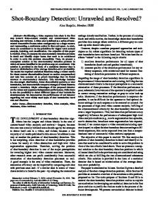
in which d(t) =k I(t + 1) − I(t) k is the pixel-to-neighbor image difference between two adjacent frames and is described in the next section, w1 is the half-width of a sliding window, and max d(t0 ) is the maximum among all image differences d(t) between adjacent frames in the sliding window, excluding the frame at time = t considered at the numerator of the expression. Therefore, when that frame is located at a maximum of d(t), the denominator selects the second maximum in the sliding window, since the first one is excluded from consideration. If the second maximum is not small, as is likely for high level of motion, then the ratio remains small. In case of a cut, there is no large second maximum, so the ratio becomes large when frame t is just past the cut. Figure 1 demonstrates the effectiveness of R(t). In this figure, there is a segment (around position c) with large motion. A series of large responses in are shown in d(t). But in R(t), these are correctly eliminated. All peaks in R(t) correspond to real cuts.
Figure 1: Effectiveness of second-max ratio criterion in detecting cuts. Note that the peaks due to motion that appear in d(t) do not appear in R(t).
2.2. Image Difference Computation There are many ways to compute the difference between two images. The following three are popular: 1. Pixel-to-pixel difference 2. Pixel-to-neighborhood difference 3. Histogram difference. We can think of the image difference as a distance between two vectors in a feature space. In the first and second methods, the features are in the pixel space, with the color of each pixel as one component of each feature. In the third method the features are in histogram space, with each histogram bin a component of each feature. The first method is not robust to motion in videos. The second method is an advanced version of the first method with a degree of motion compensation. The third method can be computed by the Euclidean distance or any other defined histogram distance in the histogram space. One of the drawbacks of the third method is that it totally discards the spatial distribution of the images. Our experiments support our analysis that the second method, pixel-to-neighborhood difference, is the best for evaluating image difference. In our implementation we compute the pixel-to-neighborhood difference as d(t) =k I(t + 1) − I(t) k= c
X i,j
(
min
k∈[i−w2 ,i+w2 ], sl∈[j−w2 ,j+w2 ]
2
(
X
m∈{R,G,B}
|Ik,l (t + 1)[m] − Ii,j (t)[m]|))
(2)
in which c is a scalar constant, w2 is the semi-width of the motion compensation searching window, Ii,j (t)[M ] is the channel value corresponding to m for the pixel position (i, j) of the frame image I(t), with m ∈ {R, G, B}.
3. Dissolve Detection In dissolve detection, we cannot use the image difference between two adjacent frames, because it is small during the dissolve. But there will be a large image difference between two frames if we skip an interval (such as a 25 frame interval). This skipping image difference can be used as a cue to dissolve detection. But it is not a unique criterion for finding a dissolve. It is very common that a peak of the skipping image difference in a sequence is not a dissolve (it can be a cut, a wipe, a shot with large motion, or the combinations of these events). Therefore we need to add other criteria for reliable dissolve detection. Another criterion we can use is the degree of linearity of a sequence of frames. This is because, in the mechanism of dissolve effect generation, most video editing processors use a linear combination of the signal before the dissolve transition (noted as signal A) and the signal after the transition (noted as signal B). Thus in this model the dissolve is a simultaneous fade-out of the signal A and fade-in of signal B. This implies that, during the dissolve transition, images change linearly. Hence the degree of linearity can be selected as another criterion to dissolve detection using its generative properties. Technically, it can be evaluated from the normalized linear error within a sequence of frames. We propose a method for dissolve detection which combines the above two criteria. Suppose we currently have a sequence of w images which is a segment in the video sequence starting with I(t) and ending with I(t + w − 1). We define the current skipping image difference value as D(t) =k I(t+w−1)−I(t) k= c
X
(
i,j
min
k∈[i−w2 ,i+w2 ],l∈[j−w2 ,j+w2 ]
(
X
|Ik,l (t+w−1)[m]−Ii,j (t)[m])) (3)
m∈{R,G,B}
We define the current normalized linear error along this part of video as Pi=w−1
LE(t) =
i=0
i i k I(t + 1) − ((1 − w−1 )I(t) + w−1 I(t + w − 1)) k k I(t + w − 1) − I(t) k
(4)
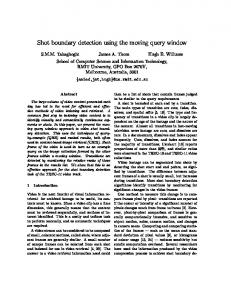
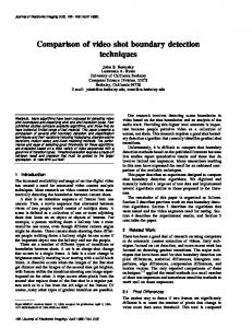
We detect a dissolve by the simultaneous presence of a peak of D(t) and a valley of LE(t). Figure 2 shows an example of detected dissolves from a news video. Here we have four dissolves that all satisfy our dissolve model. Figure 2 also illustrates that we can easily estimate the start frame number and end frame number of a dissolve transition. In Eq. 4, we use the linearity assumption in RGB color space. One concern could be that in analog television and in MPEG encoding, other color spaces are used. In which color space is the dissolve signal linear? In fact, these three color-spaces are equivalent in linearity, because there exists a linear transform between each pair of the three color-spaces. We also did some experiments to show this equivalence. For example, Figure 3 shows the LE(t) curves for RGB color space and YUV color space and their shapes are similar. In our implementation, we compute the linearity errors in the RGB color space.
4. Elimination of Flash There may be a lot of camera flash in videos, especially in news videos. A high-intensity light of very short duration is produced. Flash will cause a false alarm for cut detection, because it will increase the global brightness of one or more frames dramatically. Our method to eliminate false alarms caused by flash from candidate cuts uses the following two facts: (1) the duration of flash is very short, generally only one or two frames, (2) the images before a flash are similar to the images after the flash, if they are in the same shot. Following the method described in Section 2, we can get candidate cuts by computing R(t). These candidate cuts will be filtered by 3
Figure 2: Four dissolves with simultaneous peak of D(t) (darker red curve) and valley of LE(t) (lighter green curve) . our post-processing module to eliminate false alarms caused by flash. For a candidate cut position, noted as t, we examine the following four values: k I(t + 1) − I(t − 2) k, k I(t + 1) − I(t − 1) k, k I(t + 2) − I(t) k, k I(t + 3) − I(t) k. If any of these four values is less than a threshold, this candidate is considered to be a false alarm caused by flash, and filtered out from candidate cuts. This algorithm performs quite well in experiments, and filters out most of the false alarms caused by flash. Also notice that, in the special cases when the flashlight happens to be at the real cut boundary position, our algorithm also works. It will not filter out the cut because the images before the cut and those after the cut have large differences.
5. Merging Adjacent Fade-Out and Fade-In Fade-out and fade-in are very common in videos. Fade-out is a dissolve from an image (noted as image A) to a black frame, while fade-in is a dissolve from a black frame to an image (noted as image B). In most cases, a fade-out will be followed by a fade-in. In the framework introduced above, we will get two dissolve transitions in this case. One is the preceding fade-out, and the other is the subsequent fade-in. But this is not a reasonable output. In the shot boundary detection output, we should deliver only one dissolve from image A to image B. Therefore we have a post-processing module to merge adjacent fade-out and fade-in into one dissolve transition. In this post-processing module, for a candidate dissolve transition, we analyze the ratio of the number of black frames during the transition divided by the total number of frames of the transition. If this ratio is over 0.5, we consider the transition to be a fade-in or fade-out. We merge two such close detected fade-in / fade-out transition components to one new dissolve transition. In our implementation, a frame is declared to be a black frame if at least 90% or all the pixels are such that R < 25, G < 25 and B < 25.
4
Figure 3: LE(t) in RGB color space (left picture) and YUV color space (right picture) .
6. Implementation In our implementation, we combined our algorithms with an MPEG1 decoder. In the decoding, we keep a buffer of 25 sequential frames. It is a cyclic pointer array. Each pointer in the array is pointing to an image structure. Every time a new frame is decoded, the frame buffer is updated correspondingly and the features d(t), R(t), D(t) and LE(t) are computed based on the current frame buffer. The update rule is that the newly decoded frame comes in the buffer and pushes out the pointer for the oldest frame. The array is called cyclic because if the last decoded frame is replaced at the end of the array, the current newly decoded frame will be replaced at the start position of the array. This array is very convenient for memory management and the only overhead is a pointer pointing to the currently processed position in the buffer.
7. Experimental Results We submitted five runs to TRECVID 2004. Our run-ids are D0 , D1 , . . . , D4 . Generally, they are obtained by the same algorithms for feature extraction and shot boundary detection decision. The difference between the five runs we submitted is with the different values of parameters in our algorithms, including the w, w1 , w2 parameters introduced above, the thresholds for R(t), and the thresholds for finding the peaks of D(t) and valleys of LE(t). The results are shown in the Table below. They show the tradeoff between precision and recall. Run-id D0 D1 D2 D3 D4
Recall for all 0.802 0.816 0.809 0.846 0.731
Precision for all 0.847 0.833 0.842 0.693 0.908
Recall for cut 0.900 0.900 0.900 0.923 0.864
Precision for cut 0.877 0.880 0.877 0.733 0.921
Recall for dissolve 0.595 0.639 0.617 0.685 0.450
Precision for dissolve 0.765 0.719 0.750 0.599 0.859
Frame-recall for dissolve 0.567 0.536 0.568 0.554 0.656
Frame-precision for dissolve 0.792 0.795 0.795 0.741 0.787
As a more thorough analysis, we find that 29% of all missed gradual transitions are caused by wipes. Wipes 5
are difficult to detect effectively in videos because they are of various types and the pixel-to-neightbor image differences have different properties for different styles of wipes. We also find that 25% of all missed cut transitions are caused by extremely short dissolves. In TRECVID 2004 data, there are a lot of extremely short dissolves involving only three frames. These transitions are detected as dissolves in our submission, but in the TRECVID ground truth, they are counted as cuts.
8. Future Work Papers submitted by other participants propose different methods for doing shot boundary detection. Tsinghua University [1], RMIT University [2], and FX Palo Alto Lab [3] obtained the best results. Tsinghua University considers motion information in shot boundary detection. RMIT University proposes an impressive PrePostRatio to detect gradual transitions. FX Palo Alto Lab views shot boundary detection as a general supervised classification problem rather than an ad-hoc peak detection. All these ideas are illuminating. Combining them to our work would be helpful. Moreover, our own methods can still be improved. For example, in the current implementation, the width of the sliding window is fixed at 25 frames. An adaptive sliding window width may perform better.
References [1] Jinhui Yuan, Wujie Zheng, Zijian Tong, Le Chen, Dong Wang, Dayong Ding, Jun Wu, Jianmin Li, Fuzong Lin, Bo Zhang, “Tsinghua University at TRECVID 2004: Shot Boundary Detection and High-level Feature Extraction”. [2] Timo Volkmer, S.M.M. Tahaghoghi, Hugh E. Williams, “RMIT University at TRECVID 2004”. [3] Matthew Cooper, Ting Liu, Eleanor Rieffel, “Shot Boundary Detection Combining Similarity Analysis and Classification”, TRECVID 2004.
6