Should SDBMS Support a Join Index?: A Case study from CrimeStat Pradeep Mohan
Shashi Shekhar
Ned Levine
Department of Computer Science
Department of Computer Science
Ned Levine and Associates
University of Minnesota
[email protected]
University of Minnesota
[email protected]
Houston, TX
[email protected]
Ronald E. Wilson
Betsy George
Mete Celik
National Institute of Justice
Department of Computer Science
Department of Computer Science
Washington D.C
University of Minnesota
[email protected]
University of Minnesota
[email protected]
[email protected]
ABSTRACT Given a spatial crime data warehouse, that is updated infrequently and a set of operations O as well as constraints of storage and update overheads, the index type selection problem is to find a set of index types that can reduce the I/O cost of the set of operations. The index type selection problem is important to improve user experience and system resource utilization in crucial spatial statistics application domains such as mapping and analysis for public safety, public health, ecology, and transportation. This is because the response time of frequent queries based on the set of operations can be improved significantly by an effective choice of index types. Many spatial statistical queries in these application domains make use of a spatial neighborhood matrix, known as W in spatial statistics, which can be thought of as a spatial self-join in spatial database terminology. Currently supported index types such as B-Tree and R-Tree families do not adequately support spatial statistical analysis because they require on-the-fly computation of the WMatrix, slowing down spatial statistical analysis. In contrast, this paper argues that Spatial Database Management Systems (SDBMS) should support a join index to materialize the WMatrix and eliminate on-the-fly computation of the common selfjoin. A detailed case study using the popular spatial statistical software package for public safety, namely CrimeStat, shows that join indices can significantly speed up spatial analysis such as calculation of Ripley’s K and identification of hotspots.
Keywords Join Index, Spatial Statistics, W Matrix, Self-Join
1. INTRODUCTION Given a spatial crime data warehouse that is updated infrequently and a set of operations, the spatial index type selection problem is to find a set of spatial index types that can reduce the I/O cost of the set of operations under given constraints of storage and update overheads. The index type selection problem is important to improve user experience, response time, and system resource utilization. For example, in tools such as CrimeStat[6], the response time for identification of hotspots is 2 hours for a dataset size of 15000 crime reports. This slow response time occurs because CrimeStat is a main memory tool. Using spatial index types e.g., a join index family, may lower the response time to a few minutes, thereby enhancing the user experience.
Categories and Subject Descriptors H.2.2[PHYSICAL DESIGN]: Access methods
General Terms Design, Experimentation Figure 1: Identification of Hotspots Permission to make digital or hard copies of all or part of this work for personal or classroom use is granted without fee provided that copies are not made or distributed for profit or commercial advantage and that copies bear this notice and the full citation on the first page. To copy otherwise, or republish, to post on servers or to redistribute to lists, requires prior specific permission and/or a fee. ACM GIS '08 , November 5-7, 2008. Irvine, CA, USA (c) 2008 ACM ISBN 978-1-60558-323-5/08/11...$5.00
This paper focuses on spatial statistical queries in the context of mapping and analysis for public safety. The application considers questions such as, "Are there spatial concentrations of crime that warrant increased police targeting at the community, city, and county levels?" to identify a set of spatially grouped instances defined as hotspots. For example, Figure 1 illustrates the identification of burglary hotspots in applications such as mapping and analysis of public safety. In these scenarios, law
enforcement agencies normally have very limited resources such as officers and patrol vehicles to deploy in a concentrated manner. Given a large area such as a city, it would be very useful for law enforcement agencies to examine different possible configurations for distributing their limited resources to areas where there is increased crime activity. To perform this strategic placement, crime analysts and law enforcement agencies perform an exploratory analysis. Similar spatial statistical queries are important in many other application domains such as public health, transportation, ecology, consumer applications etc. For example, public health authorities may be interested in hotspots of diseases such as cancer clusters [14] in order to identify and remedy environmental factors such as contaminated soil or water. Transportation professionals may be interested in identifying and remedying spatial concentrations of traffic accidents by re-designing transportation networks via traffic calming etc. Ecologists may identify spatial concentrations of endangered species to promote their protection. Many of these queries make use of a spatial neighborhood matrix known as W in spatial statistics and perform repeated W Matrix computation for different neighborhoods. We call such queries W-Queries. Current spatial database management systems (SDBMS) provide a rich set of operations and spatial index structures such as B-Tree and R-Tree index families that can enhance the efficiency of processing queries in various applications [1, 3, 4, 10, 11, 12, 17]. However, these SDBMS must perform repeated on-the-fly computation of the W-Matrix and are limited in their ability to support W-Query operations. This paper argues that SDBMS should support a self-join index. The paper aims to establish the utility of the join index to process W-Queries efficiently by evaluating the idea of a self-join index. Related Work: Research related to the index type selection problem can be classified into two categories: (1) spatial indices that make use of on-the-fly join computation strategies by computing joins as a part of the query evaluation process, (2) spatial indices used for direct(lookup) join computation that compute joins by performing a sequence of lookups. On-the-fly join computation techniques that are based on spatial indices, namely the R-Tree and its variants, are suitable for computing the spatial join for a single neighborhood relationship [1, 3, 4, 5, 6, 7, 8, 10, 11, 17, 18, 19]. However, W-Queries are exploratory in nature and require repeated self-join computation, making on-the-fly join computation expensive. Spatial indices such as R-Tree and its variants, Quad tree, Grid Files, etc., have been incorporated as a part of commercial SDBMS systems [7, 8, 9, 19, 16]. IBM Informix Spatial DataBlade makes use of the R Tree, ESRI Arc SDE makes use of Grid Files, Oracle spatial makes use of R Tree and Quad tree, and Microsoft SQL Server 2008 spatial data support makes use of multi-level Grid files. These commercial SDBMS tools retain the limitations of the corresponding spatial indices and hence do not provide support for W-Queries and their operations. A major issue faced by existing SDBMS tools to support several spatial indices is that the choice of a spatial index type for a given set of workloads affects the strategy for I/O optimization, query optimization strategies, concurrency control, and recovery strategies.
Direct join computation techniques are based on spatial indices such as the (spatial) join index [8,13]. Join indices have been primarily used in the context of computing a spatial join between two different relations to speed up online query processing infrequently updated databases. However, current join indices are represented as bi-partite graphs [9, 14]. By contrast, W-Queries are primarily focused on computing several spatial self-join operations. In self-join cases, the join index becomes a neighborhood graph rather than a bi-partite graph representation. Hence, the current representation of join indices as bi-partite graphs needs re-consideration. Our Contributions: First, we characterize the computational structure of W-Queries. We consider the computation of Ripley's K Function, and the identification of hotspots [2,6] for modeling W-Queries. We propose a set of operations for handling these queries. We define the spatial index selection problem for handling the set of operations efficiently. We propose two variants of the self-join index namely: (a) the Self-join Edge List Index (SJELI) and (b) the Self-join Adjacency List Index (SJALI). We also propose algorithms for processing W-Queries. We evaluate the I/O efficiency of the proposed variants of the self-join index using algebraic cost models for the operations. The cost model and the experimental results establish the utility of the self-join indices. Experimental results using real crime datasets indicate that the self-join indices decrease the user response time of W-Queries by a factor 40 compared to a single threaded version of CrimeStat and outperform an R-Tree based Tree Matching self-join algorithm. Based on these findings we believe that existing SDBMS should adopt the self-join indices to support spatial statistical queries such as W-Queries. Scope: This paper primarily focuses on the selection of a suitable index type for a given set of operations. The join indices are materialized for the study area, a primary requirement in most spatial statistical analysis applications. Our propositions are mainly focused on multiple spatial neighborhood analysis queries within a particular study area. The aim is to reduce the response time of the proposed set of operations for W-Queries in a spatial crime data warehouse setting. We understand that adding new index types in a SDBMS is a complex decision due to the impact on issues such as concurrency control, recovery, and evaluation of storage costs. These issues are beyond the current scope of the paper. Outline: The rest of the paper is organized as follows. Section 2 presents the basic concepts and the spatial index type selection problem. Section 3 describes the proposed self-join index variations and design decisions. In Section 4, we propose two algorithms for two example W-Queries, e.g., Ripley's K Function computation and identification of hotspots, and propose an algebraic cost model for the set of W-Query operations. The experimental evaluation is given in Section 5 and Section 6 outlines the conclusions and future work.
2. Basic Concepts and Problem Statement In this section, we present some basic concepts required to model W-Queries. We model W-Queries by identifying two example queries, namely the computation of the Ripley KFunction and the identification of hotspots. We propose a set of W-Query operations based on the example queries and characterize their computational structure.
N3
N3 N2
N2 N7
N1
N6
N3 N7
N1
N3
N6
N2 N2
N5
N5
N7
N1 N4
N4
(a )
(b )
N7
N1
N6
N6 N5
⎡N 7 ⎢N 6 ⎢ ⎢N 5 ⎢ ⎢N 4 ⎢N3 ⎢ ⎢N 2 ⎢ N1 ⎢ ⎣⎢
0 0
0 1
0 0
0 1
0 1
1 0
1 0 1
1 0 1
0 0 0
1 0 0
0 1 0
1 1 0
1 0 N1
0 1 N2
1 1 N3
0 0 N4
1 1 N5
1 0 N6
(c )
0 ⎤ 1 ⎥⎥ 0 ⎥ ⎥ 0 ⎥ 0 ⎥ ⎥ 0 ⎥ 0 ⎥ ⎥ N 7 ⎦⎥
⎡N 7 ⎢N 6 ⎢ ⎢N 5 ⎢ ⎢N 4 ⎢N3 ⎢ ⎢N 2 ⎢ N1 ⎢ ⎣⎢
N5
0
0
1
1
0
1
1
1
0
1
1
0
1
1
1
1
0
1
1
0
0
0
1
1
1 1
1 0
0 1
0 0
1 1
0 1
0
1
1
1
1
1
N1
N2
N3
N4
N5
N6
0 ⎤ 1 ⎥⎥ 0 ⎥ ⎥ 1 ⎥ 1 ⎥ ⎥ 0 ⎥ 0 ⎥ ⎥ N 7 ⎦⎥
(d )
N4
Neighbor Relation R1 Neighbor Relation R2 (a)
Figure 2: Sample dataset and the W-Matrix for different relations. (a) Neighborhood graph for neighborhood relation R1, (b) Neighborhood graph for relation R2. (d) W-Matrix for relation R1. (f) W-Matrix for relation R2.
In spatial statistics, the W-Matrix is a matrix--based representation of space and a measure of the adjacency, proximity, distance or level of spatial interaction between spatial instances [3]. Given a uniform spatial framework and a set of spatial instances, W-Queries re-compute the W-Matrix for different neighborhood relations. For example: Figure 2a and 2b represent the spatial neighborhood graph for a spatial dataset. Figure 2a corresponds to a neighborhood relation R1, and Figure 2b corresponds to a neighborhood relation R2. The corresponding W- Matrices for the neighborhood graphs is illustrated in Figure 2c and 2d respectively. Spatial instances are represented by N1, N2…,N7 in a uniform spatial framework. In the W-Matrix, a 1 denotes that the two spatial instances satisfy the neighborhood relation and a 0 denotes that the two spatial instances do not satisfy the neighborhood relation. Definition 2.1 Given two spatial instances Si, and Sj , where i ≠ j, in a spatial dataset SD a neighborhood relation R(Si, Sj) can be defined as a measure of spatial interaction, distance or adjacency. For example, In Figure 2, R1 and R2 are two different spatial neighborhood relations. Definition 2.2 Given a spatial framework S, the W-Matrix is defined as a set of values that quantify the spatial interaction, distance or adjacency. These values can be binary or real depending on the measure of spatial interaction used. Formally, the W-Matrix can be defined as follows[13];
W ( S D , R ) = { R ( S i , S j ) | ∀ S i , S j ∈ S D and R ( S i , S j ) is valid and i ≠ j} Definition 2.3 Given a spatial instance Si , the no_of_instances(Si , R) of instance Si is the number of spatial instances Sj є SD , i≠j, that satisfy the neighbor relation R. For example, in Figure 2, R1, R2 are two different spatial neighborhood relationships whose no_of_instances(N1,R1) = 3 and no_of_instances(N2,R2) = 4 Definition 2.4 Given a spatial instance Si , the average edge weight (AEW) (or average weight) of a spatial instance is the sum of the values of R(Si , Sj ) divided by the Frequency(Si ,R) where Sj є SD and i≠j, that have a valid neighbor relation R. The term average edge weight is relevant only if the neighbor relation represents a value of distance or similarity.
N4
Neighbor Relation R1 Neighbor Relation R2 (b)
Figure 3: Computational structure of W-Queries. (a) Ripley's K (b) Hotspots
2.1 Two Simple W Queries To model W-Queries, we consider two spatial statistical queries that have been applied to compute statistics in CrimeStat[6]. Query I: Is data spatially clustered ?. Query I relates to the calculation of a well-known statistical measure called Ripley's K function [2, 14]. This measure calculates the cumulative number of spatial instances that are within a search radius of each spatial instance in the dataset. This cumulative count is computed for different neighborhood radii. Figure 3(a) illustrates the method of computing Ripley’s K Function. In the figure, dark circles around the spatial instances N1, N2.., and N7 represent neighborhood relationship R1, and dashed circles around the spatial instances represent neighborhood relationship R2. The Ripley K Function method computes the number of spatial instances around a particular spatial instance for a particular neighbor relation R2 and reports the cumulative sum of these frequencies over all spatial instances. The process is repeated after the neighbor relation is changed to R1 and so on until a significant number of levels are completed. The number of neighborhood relationships is of the order of 100 in spatial statistics tools such as CrimeStat [6]. Query II: Are there concentrations of crime that warrant increased police targeting at the community, city, and county level? Query II relates to the identification of a spatially grouped set of instances defined as hotspots. Figure 3(b) illustrates hotspots that can be extracted from the spatial dataset for multiple neighborhood definitions. N1, N2…and N7 are the spatial instances. In the figure, dark ellipses refer to hotspots that are identified for a neighborhood R1 and the dashed ellipse refers to hotspots that are identified for a neighborhood R2. The computational process begins with the computation of the W-Matrix for an initial neighborhood relation R and the selection of a set of representative points called seeds. Seeds are defined as spatial instances which have a minimal edge weight compared to their neighbor spatial instances. For example, in Figure 3(b), N2, N5, and N6 are the seed points since they have minimum average edge weights? for the neighbor relation R1. The hotspot identification process always maintains a list of potential seeds that are updated whenever a new hotspot is identified. The key challenge in the process is to identify nonoverlapping hotspots so that spatial instances are not reconsidered in subsequent hotspots.
Table 1: W-Queries from CrimeStat[6] Statistic W(SD,R) Consecutive
Frequency
Average Edge
Join Computation:
Join Computation:
W Subsets
Based
Weight Based
On the Fly
Look up
Ripley's K Function
Yes
Yes
Yes
NO
NO
Yes
Nearest Neighbor Statistic
Yes
Yes
Yes
NO
NO
Yes
Hotspots
Yes
Yes
Yes
Yes
NO
Yes
Moran’s I
NO
NO
NO
NO
Yes
Yes
Geary’s C
NO
NO
NO
NO
Yes
Yes
Local Moran (LISA)
Yes
NO
NO
NO
NO
Yes
2.2 Case Study: W Queries from CrimeStat Spatial statistical queries that can be classified as W-Queries and that mainly involve repeated computation of neighborhood relationships are drawn from crime analysis tools such as CrimeStat [6]. Table 1 lists some of these queries. CrimeStat has several spatial autocorrelation routines including Moran’s “I”, Geary’s “C” and LISA. These are global level statistics that determine if there is clustering or dispersion within a dataset across a study area. They are used as a guide to conduct local level hotspot analysis whereby if the results indicate there is no clustering or dispersion, then any hotspots found with local level techniques will likely be false positives. These spatial statistical measures can also be modeled as W-Queries.
2.3 Operations for W-Queries W-Queries can be modeled as a set of operations that can be used to identify a suitable spatial index type to process them efficiently. Figure 4 illustrates the effect of the set of operations on the example dataset illustrated by Figure 1. Since the spatial dataset is modeled as a neighborhood graph under a neighborhood relation, we make use of terminology used in the spatial network database literature such as predecessor and successor [17]. We make use of node coloring to distinguish a predecessor from a successor as the operations are applied on a neighborhood graph.
get-successor (Si): Retrieve the farthest unreported successors of Si. This operation returns the spatial instance which is the successor of Si and has the maximum value of the neighbor relation R with Si. We call this the "farthest successor first " strategy. For example: Figure 4(c) shows the effect of the get-successor(Si) operation on the spatial instance N2, where the instances N1, N3, N5, and N6 are reported as successors since they have the same color as that of N3. get-predecessors (Si): Retrieve the predecessors of Si. Retrieves the spatial instances that have a color different from that of spatial instance Si . This operation is executed normally when the degree of spatial instances requires updating. For example: Figure 4 (f), shows the result of get-predecessors(Si) on the spatial instance N2. The operation reports instances N5 and N6 as the results. get-predecessor-of-successor (Si): Retrieve the predecessors of the successor of Si This operation returns the nearest uncolored spatial instance to the successor of Si. A predecessor is a spatial instance Sj that does not have the same color as spatial instance Si.
get-neighbors-in-relationship(Si,R): Identify the neighbors of a spatial instance Si.
For example: Figure 4(d) shows the result get-predecessor-ofsuccessor(Si) applied two times on the spatial instance N2. The operation reports instances N4 and N7 as the results.
Given the spatial instance Si, the get-neighbors-in-relationship() operation colors the spatial instance Si and gives all the neighbors that satisfy the relationship R the same color as Si.
get-predecessors-of-successor (Si): Retrieve the predecessors of the successors of Si.
For example: Figure 4 (a) shows the effect of the get-neighborsin-relationship(Si,R) on the spatial instance N2 where the operation get-neighbors-in-relationship(N2,R) results in the coloring of the instances N2, N3,N5 and N6.
This operation retrieves the predecessors of the successor of a spatial instance Si. This operation is important to update the average edge weight of neighboring spatial instances of the neighbors of Si.
get-successors (Si): Retrieve the successors of Si.
For example: Figure 4(g) shows the result of this operation on the spatial instance N2,where the first successor of N2 is N1 and its first predecessor is N5 gets reported.
The successor of a spatial instance Si is defined as a set of spatial instances that satisfy the neighbor relation R with Si and have the same color. For example: Figure 4 (b) shows the effect of the getsuccessor(Si) operation on the spatial instance N2, where the instances N1, N3, N5, and N6 are reported as successors since they have the same color as N3.
update-successors (Si, ): Un-colors all the successors of Si Checks whether the spatial instance Si is colored; if it is colored then it un-colors the spatial instance. represents a list of successors to be updated.
N3
N3 N2 N7
N1
N7 N6
N5
N4
N4
(a)
(b)
N7
N5
N4
N4
(d)
N3
N3 N2
N7
N1
N2 N7
N1
N6
N6
N5
N6
(c)
N2 N6
N7
N1
N6 N5
N3 N2
N1
N7
N1
N5
N3
N2
N2
N1
N6
N3
N3 N2
N5
N5
N7
N1
N6 N5
N4
N4
N4
N4
(e)
(f)
(g)
(h)
C olored S patial Instances
U nm arked Instance
R1
S uccessors
R equires U pdate
R2
P redecessors
Figure 4 Effect of W-Query operations on sample dataset. (a)get-neighbors-in-relationship(N2,R1). (b) getsuccessors(N2). (c) get-successor(N2) (d)get-predecessor-of-successor(N2) applied two times. (e) updatesuccessors(N2). (f) get-predecessors(N2).(g) get-predecessors-of-successor(N2). (h) get-predecessor(N2).
For example: Figure 4 (e) shows the result of updatesuccessors(Si) on the spatial instances N5 and N6. update-average edge weight (Sj): Update the average edge weight of a spatial instance. This operation updates (reduces) the average edge weight of a given spatial instance Si. For example: This operation is applied on the instances N5 and N6, which are shown in Figure 4(f,g). N5 is updated two times in this example.
2.4 Problem Statement This section defines the spatial index type selection problem given a set of operations that are relevant to W-Queries. Given: •
A spatial crime data warehouse
•
A set of operations O
Find: •
3. Self-Join Index and Its Variants In this section, we formally define a self-join index (SJI) and propose two variants, namely the Self-Join edge list index (SJELI) and the Self-join adjacency list index (SJALI). We formally define the self-join index as:
SJI = {< S i , S j , R ( S i , S j ) >| ∀S i , S j ∈ S D & (∃R ∈ R S , R ( S i , S j ) is valid ) & i ≠ j} where SD is the spatial dataset, RS is a set of neighborhood relationships that are defined for a spatial framework S. For example: From Figure 5, RS = {R1,R2}. R(Si ,Sj ) is either R1 or R2.
A suitable secondary memory index structure type.
Objective: •
minimizes the I/O cost of the operations get-neighbors-inrelationship(), get-successors() and the user response time of the W-Query. Different W-Queries may have different workloads which are provided as an input to the query. For example, Ripley's K has parameters such as maximum neighborhood size and number of spatial neighborhoods.
To minimize the I/O cost of the set of operations O.
Constraints: •
Spatial datasets are updated infrequently.
•
Concurrency control and recovery considerations are addressed separately.
•
There are no storage overheads.
•
User response time is minimized.
Example: To compute a W-Query such as the Ripley K Function, given a spatial dataset and a set of operations, namely getneighbors-in-relationship() and get-successors(). The objective of the above problem is to find a suitable spatial index type that
3.1 Representations of the SJI Traditionally, the join index has been represented as a bipartite graph. Since W-Queries repeatedly compute self-joins, the modeling of the self-join index as a bi-partite graph needs to be modified to that of an undirected neighborhood graph, G=(SD, E). The neighborhood graph G consists of a set of spatial instances SD and an edge set E. Each element SiєSD is a spatial location in a uniform spatial framework S. The set of edges E is a subset of the cross product, S D × S D . Each element (Si, Sj ) in E is an edge that joins instances Si, and Sj, where i≠j. Also each edge has a weight which is the level of spatial interaction, distance or adjacency.
Figure 5: Self-join index representations.(a). Neighborhood graph for relation R1.(b). Neighborhood graph for relation R2.(c) Self-join edge list index (SJELI).(d). Self-join adjacency list index.(SJALI)
This neighborhood graph can be represented in two different ways, namely, the edge list and the adjacency list. Figure 5(a) and 5(b) are the neighborhood graphs for the relations R1 and R2 respectively. We present the design of the two representations and evaluate the effect of the operations on the two variants. 3.1.1 Self – Join Index: Edge List Representation (SJELI) The edge list representation of the self-join index is illustrated in Figure 5(c). In this representation, the join index is ordered by column 1 and within column 1 by the value of the relation R(Si,Sj). This representation does not provide any information on the successors or the predecessors of a spatial instance Si. This is clearly evident from its representation. A clear challenge with this representation is to determine an optimal partitioning of the SJELI to minimize the I/O costs of the set of operations. 3.1.2 Self – Join Index: Adjacency List Representation(SJALI) The adjacency list representation of the self-join index is illustrated in Figure 5(d).The adjacency list representation has clear advantages compared to that of the edge list representation. First, the adjacency list representation maintains a list of successors and predecessors that are critical for processing WQueries. Second, the coloring scheme used by the set of operations can easily exploit the adjacency list representation to retrieve the successors or predecessors with lesser I/O. Also, processing updates on the adjacency list is easier due to the same reasons. 3.1.3 Design Issues We make use of the connectivity clustering heuristic [17] to cluster the spatial instances of the SJALI and SJELI. CCAM (Clustered Connectivity Access Method) [17] makes use of
separate lists for successors and predecessors and does not exploit the concept of a spatial neighborhood. The self-join indices, SJALI and SJELI are primarily neighborhood graphs that are represented as adjacency lists and edge lists. We apply the connectivity clustering heuristic for the two neighborhood graphs to store them into disk pages. In the design of the SJALI, we maintain only one list of adjacent neighbors of a particular spatial instance. The proposed set of W-Query operations, for example, getneighbors-in-relationship(Si,R), makes use of a coloring heuristic to retrieve the successors and the predecessors of a particular spatial instance. To allocate these spatial instances to disk pages,we make use of the same connectivity clustering heuristic on the neighborhood graph. For example, in Figure 4(d), a typical page allocation would involve storing N1, N2, and N3 in the same page; N4,N5, and N6 in another page; and N7 in a separate page. This allocation scheme changes with the maximum size of a page and the value of the Connectivity Residue Ratio (CRR) [17]. CRR is defined as the probability that two neighboring spatial instances are present in the same disk page. Utilizing the same heuristic on the SJELI involves storing the edge lists of spatial instances in the same disk page such that the number of cut edges is minimized. This allocates the edge lists of spatial instances to pages where each edge of the spatial instance corresponds to a page entry. In some cases for large neighborhood sizes, it is possible that the edge list of one spatial instance itself may exceed one single page. For example, in Figure 5(c), a typical page allocation would involve allocating the edge lists of N1, N2, and N3 to the same page, edge lists of N4,N5, and N6 to another page, and N7 to a separate page.
Table 2: Trace of CalcRipleyK Algorithm The key trade-off in the two different representations is in the value of the connectivity residue ratio (CRR) they yield. . The SJELI would yield a lower value of CRR for small page sizes, thus resulting in larger I/O costs. SJELI would also incur more I/O costs for larger neighborhood sizes than the other representation. This clearly indicates that the value of the CRR in the case of both the SJELI and the SJALI depends on the value of the neighborhood relation R. An in-depth evaluation of the variation in CRR for the two self-join indices is beyond the scope of this paper.
Neighbor get-neighbors-inRelation relationship(Si, R)
get-successors(Si)
Frequency
R2
[N3,N1,N5,N6]
4
N2:[N3,N1,N5,N6]
N1:[N2,N3,N5,N4,N6] [N2,N3,N5,N4,N6] 5
Algorithm 1: CalcRipleyK: Computation process for computing Ripley’s K Function Inputs: •
Spatial sataset SD, Query: Is data spatially clustered?,
•
Total number of levels, Study Area
Output: •
2. 3.
do begin for every spatial instance Si in SD
4.
get-neighbors-in-relationship(Si,R[i])
5.
F[i] := F[i]+size(get-successors(Si,R[i]))
6.
update-successors(Si)
7.
N4:[N5,N6,N7,N1]
[N5,N6,N7,N1]
4
N6:[N7,N5,N4,N1]
[N7,N5,N4,N1]
4
N7:[ N6,N4,N3]
[ N6,N4,N3]
3
R1
N2:[N3,N1,N5,N6]
[N3,N1,N5,N6]
4
N1:[N2,N3,N5,N6]
[N2,N3,N5,N6]
4
N3:[ N2,N1]
[ N2,N1]
2
N4:[N5,N6]
[N5,N6]
2
N5:[ N4,N6,N2,N1]
[ N4,N6,N2,N1]
4
N6:[N7,N5,N2 ]
[N7,N5,N2 ]
3
N7:[N6 ]
[N6 ]
1 Total = 20
4.2 Identification of Hot Spots The identification of hotspots involves the use of the operations get-neighbors-in-relationship(Si,R), getsuccessors(Si,R), get-successor(Si), update-successors(Si), getpredecessors(Si), and update-average-edge-weight(Si). Algorithm 2, Hotspot_JI lists the computational process for the identification of hotspots. Algorithm 2: Hotspot_JI: Computation process for extracting hotspots from a spatial dataset. Inputs:
K – Function: Measure of spatial randomness.
Procedure: CalcRipleyK 1.
4
Total = 28
4.1 Ripley's K Function Computation The Ripley K Function computation involves the use of two operations, get-neighbors-in-relationship(Si,R) and getsuccessors(Si). Algorithm 1 lists the computational process for the Ripley K Function. The trace of the algorithm is listed in Table 2.
[ N2,N1,N5,N7]
N5:[N4,N6,N2,N1,N3 ] [N4,N6,N2,N1,N3 ] 5
4. W-Query Processing Algorithms In this section, we propose two query processing algorithms using the set of operations get-neighbors-in-relationship(), getsuccessors(), get-predecessors(), get-successor(), getpredecessor(), get-predecessor-of-successor(), get-predecessorsof-successor(), update-average-edge-weight(), and updatesuccessors(). These operations are used to design the algorithms for W-Queries, namely Ripley's K- Function computation and identification of hotspots.
N3:[ N2,N1,N5,N7]
Spatial Dataset SD, Query: Are there concentrations of crime that warrant increased police targeting at the block ,city and county level? HotspotSizeThreshold, Set of Neighbor Relations Output: Set of hotspots corresponding to each neighbor relation Procedure: Hotspot_JI 1. While ( Size(HotspotQueue >= HotspotSizeThreshold ) 2. begin
endfor
3.
8.
K [i] := calculate_ripley_k from F[i]
4.
Si := Retrieve New Seed
9.
i:= i+1
5.
get-neighbors-in-relationship(Si,R)
6.
Successor_List:= get-successors(Si)
10.
R [i] := decrease_neighborhood(R[i-1])
7.
while(R[i](predecessor-of-successor(Si))