SHRINK: A Structural Clustering Algorithm for Detecting Hierarchical ...

SHRINK: A Structural Clustering Algorithm for Detecting Hierarchical Communities in Networks Jianbin Huang

Heli Sun

Jiawei Han

School of Software Xidian University Xi’an, China

Dept. of Computer Science and Technology Xi’an Jiaotong University Xi’an, China

Hongbo Deng

[email protected] Yizhou Sun

Dept. of Computer Science University of Illinois at Urbana-Champaign Urbana, IL, USA



School of Computer Science and Technology Xidian University Xi’an, China

[email protected]

[email protected]

[email protected]

[email protected] Yaguang Liu

[email protected]

ABSTRACT

General Terms

Community detection is an important task for mining the structure and function of complex networks. Generally, there are several different kinds of nodes in a network which are cluster nodes densely connected within communities, as well as some special nodes like hubs bridging multiple communities and outliers marginally connected with a community. In addition, it has been shown that there is a hierarchical structure in complex networks with communities embedded within other communities. Therefore, a good algorithm is desirable to be able to not only detect hierarchical communities, but also identify hubs and outliers. In this paper, we propose a parameter-free hierarchical network clustering algorithm SHRINK by combining the advantages of density-based clustering and modularity optimization methods. Based on the structural connectivity information, the proposed algorithm can effectively reveal the embedded hierarchical community structure with multiresolution in largescale weighted undirected networks, and identify hubs and outliers as well. Moreover, it overcomes the sensitive threshold problem of density-based clustering algorithms and the resolution limit possessed by other modularity-based methods. To illustrate our methodology, we conduct experiments with both real-world and synthetic datasets for community detection, and compare with many other baseline methods. Experimental results demonstrate that SHRINK achieves the best performance with consistent improvements.

Algorithms, Design, Performance

Categories and Subject Descriptors H.2.8 [Database Applications]: Data Mining; G.2.2 [Graph Theory]: Graph Algorithms; I.5.3 [Clustering]: Algorithms

Permission to make digital or hard copies of all or part of this work for personal or classroom use is granted without fee provided that copies are not made or distributed for profit or commercial advantage and that copies bear this notice and the full citation on the first page. To copy otherwise, to republish, to post on servers or to redistribute to lists, requires prior specific permission and/or a fee. CIKM’10, October 25–30, 2010, Toronto, Ontario, Canada. Copyright 2010 ACM 978-1-4503-0099-5/10/10 ...$10.00.

Keywords Hierarchical Community Discovery, Graph Clustering, Hubs and Outliers

1.

INTRODUCTION

Nowadays, many real-world networks possess intrinsic community structure, such as large social networks, Web graphs, and biological networks. A community (also referred to as a module or cluster) is typically thought of a group of nodes with dense connections within groups and sparse connections between groups as well. Detecting communities in a network can provide insight into how network function and topology affect each other and has received a great deal of attention in recent years. For example, communities in a co-authorship network might imply researchers working together with the same interests, and communities in a citation network might indicate related papers on a single topic, meanwhile communities on the Web graph might represent pages of related topics. Finding communities in complex networks is a nontrivial task, since the number of communities in the network is typically unknown and the communities are often of unequal size or density. Moreover, it has been shown that there is a hierarchical structure of complex networks with communities embedded within other communities. Essentially, small communities group together to form larger ones, which in turn group together to form even larger ones [16]. Taking the co-authorship network extracted from DBLP in Figure 1 as an example, a research field can be composed of many research groups with the same academic interests. For example, there are many groups in DM research field, while a group may consist of several subgroups like “data stream mining”, “graph mining”,“mining moving object” and so on. Besides the general nodes that are densely connected with communities, there are some special nodes like hubs (denoted as red diamonds) and outliers (denoted as white triangles) in Figure 1. For example, some researchers, like “Ji-

comes not only sensitive threshold problem of densitybased clustering algorithm, but also the resolution limit that other modularity-based algorithms suffer from. The rest of the paper is organized as follows. First we briefly review some related work in Section 2. In section 3, we formulize the notion of hierarchical structural-connected clusters. In section 4, we describe the algorithms in detail. In section 5, we report the experimental results. Finally, we summarize our conclusions and suggest future work in section 6.

2.

Figure 1: Community structure and node roles for an example of co-authorship network extracted from DBLP. awei Han” and “Philip S. Yu”, have published a large amount of papers in collaboration with people from various research communities. These nodes should be considered as hubs that are closely related to different communities, forming overlapping communities. As we know, hubs play special and important roles in many real-world networks. For example, hubs in the WWW could be utilized to improve the search engine rankings for relevant authoritative Web pages [14], and hubs in viral marketing [7] and epidemiology [5] could be central nodes for spreading ideas or diseases. Furthermore, there are some nodes that are marginally connected with the community members, such as the white triangles in Figure 1. In reality, a visiting scholar who only publishes one paper with researchers in the hosted group should not be considered as a member of the group, and meanwhile it is better to be regarded as an outlier. Since outliers have little or no influence in a community, they may be isolated as noise in the network. Therefore, how to detect hierarchical communities as well as hubs and outliers in a network becomes an interesting and challenging problem. However, most existing approaches only study the community detection without considering hubs and outliers. In this paper, we propose a parameter-free hierarchical network clustering algorithm SHRINK by combining the advantages of densitybased clustering and modularity-based methods. The main contributions are summarized in the following: 1. We propose a novel parameter-free network clustering algorithm. Through shrinkage of the local microcommunities into super-node iteratively, our algorithm does not only reveal the meaningful hierarchical community structure in networks, but also identify the hubs and outliers. 2. Our algorithm can find the communities with various densities. Moreover, the clustering result does not depend on the order of processed nodes. Experimental results show that our algorithm is effective and efficient. 3. By combining the advantages of density-based clustering and modularity optimization, our algorithm over-

RELATED WORK

Community discovery in complex networks has been studied for years in multiple fields, particularly computer science and physics. Traditional graph partitioning methods, such as Kernighan-Lin algorithm [13], Girvan-Newman algorithm [11], normalized cut [24], and spectral bisection methods [25] have been widely applied to find network communities. Recently, significant progress has been archived in this research field and many approaches have been presented for detecting communities in networks. Modularity-based methods: For evaluating the quality of network partitions, Newman and Girvan proposed the modularity measure Q [20] which has been widely used in community discovery. Modularity-based methods assume that high values of modularity indicate good partitions. But it has been proven that modularity optimization is an NPcomplete problem. Most of the modularity-based algorithms find good approximation of the modularity maximum with high computational complexity such as SA (Simulated Annealing) [12], FN [19], and CNM [6]. Recently, Blondel et al. proposed a greedy modularity-based algorithm, called BGLL[3], for finding communities in weighted networks. This algorithm has a low computational complexity and can discover hierarchical communities. However, the results of the algorithm depend on the order in which the nodes are visited. Actually, the methods of greedy optimization of modularity often tend to form large communities through combination of small ones. Recent research shows that modularity is not a scale-invariant measure, and hence, by relying on its maximization, detection of communities smaller than a certain size is impossible. This serious problem is famously known as the resolution limit of modularity-based algorithms [10]. Compared with the traditional modularitybased methods, our work use the modularity as a quality function to guide the selection of optimal hierarchical communities. Hierarchical and Overlapping methods: In the presence of hierarchy, the concept of community structure becomes richer. Agglomerative or divisive hierarchical clustering are well-known techniques to solve this problem [19, 11]. Starting from a partition in which each node is its own community, or all nodes are in the same community, one merges or splits clusters according to a topological measure of similarity between nodes. In this way, one builds a hierarchical tree of partitions. Though this type of methods naturally produces a hierarchy of partitions, it needs a metric to stop the algorithm. Recently, some work focused on the problem of identifying meaningful community hierarchies [23] and detecting multiresolution levels [2, 16, 22]. The issue of finding overlapping communities has become a hot topic. Palla et al. proposed a clique percolation

3. DENSELY CONNECTED HIERARCHICAL COMMUNITIES The goals of our algorithm are not only to cluster networks hierarchically but also to identify two kinds of special nodes: hubs and outliers. Therefore, local connectivity structure of the network is used in our optimal clustering. In this section, we formalize some notions and properties of the hierarchical structure-connected clusters. Definition 1. (Structural Similarity) Let G = (V, E, w) be a weighted undirected network and w(e) be the weight of the edge e. For a node u ∈ V , we define w({u, u}) = 1. The structure neighborhood of a node u is the set Γ(u) containing u and its adjacent nodes which are incident with a common edge with u : Γ(u) = {v ∈ V |{u, v} ∈ E} ∪ {u}. The structural similarity between two adjacent nodes u and v is then ∑ w(u, x) · w(v, x) x∈Γ(u)∩Γ(v)

σ(u, v) = √ ∑

x∈Γ(u)

w2 (u, x) ·

√ ∑ x∈Γ(v)

. w2 (v, x)

(1)

1 0.8

Similarity

method (CPM) [21]. A complete sub-graph of k nodes, called k-clique, is rolled over the network through other cliques with k − 1 common nodes. In this way, a set of nodes can be reached, which is regarded as a community. One node can belong to more than one community; therefore, overlaps naturally occur. The CPM algorithm is limited by its assumption that the graph has a large number of cliques. Furthermore, the method is not suitable to detect hierarchical structure. Recently, Nepusz et al. considered the problem of fuzzy community detection in networks, which expands the concept of overlapping community structure [18]. Every node is allowed to belong to multiple communities with different degrees of membership. A measure was introduced to identify regular nodes in a community, hubs that have significant membership in more than one single community, and outliers that do not belong to any of the communities. In real networks, communities are usually both hierarchical and overlapping. Most existing methods investigate these two phenomena separately. Our work is one of the few methods that try to discover both hierarchical communities and overlapping nodes in a given network. Density-based methods: Density-based clustering approaches (e.g., DBSCAN [8] and OPTICS [1]) have been widely used in data mining owing to their ability of finding clusters of arbitrary shape even in the presence of noise. Recently, Xu et al. proposed an efficient structural network clustering algorithm SCAN [26] through extension of the DBSCAN [8]. This algorithm can find communities as well as hubs and outliers in a network. However, it requires a minimum similarity parameter ε and a minimum cluster size µ to define clusters, and is sensitive to the parameter ε which is difficult to determine automatically. To deal with this problem, Bortner et al. proposed a new algorithm, called SCOT+HintClus [4], to detect the hierarchical cluster boundaries of network by extending the algorithm OPTICS [1]. However, it does not find the global clustering result and needs an additional pruning process to expose the reasonable hierarchical structure of the networks. Our work tries to develop a parameter-free method to explore the hierarchy of structural-connected communities with multiresolution levels in networks.

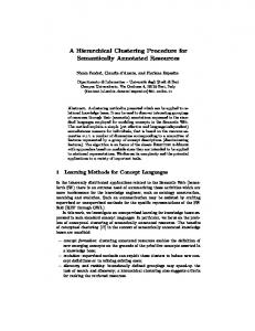
0.6 0.4 0.2 0

20

40 60 Index of Nodes

80

100

Figure 2: A segment of similarity-plot for the DBLP co-authorship network.

The above structural similarity is extended from a cosine similarity used in [26] which effectively denotes the local connectivity density of any two adjacent nodes in a weighted network. It can be replaced by other similarity definitions such as Jaccard similarity, and our experimental results show that the cosine similarity is better. The density-based clustering algorithm OPTICS [1] shows that the hierarchical cluster structure of a dataset can be obtained from the reachability-similarity values plotted for each object in the cluster-ordering. Here we intend to design a parameter-free algorithm, and we do not use the minimum similarity threshold ε and the minimum cluster size µ any more. Actually, the reachability-similarity of any adjacent nodes u and v are equal to their structural similarity when µ = 2 and the clustering results are not sensitive to the parameter µ. In Figure 2, we give a segment of ordered similarity-plot extracted from the DBLP co-authorship network. It is able to observe that the similarity distribution describes the intrinsic clustering structure accurately with high similarity regions surrounded by low similarity regions. The clusters are clearly discernible as “mountains” in the plot, and the hubs and outliers are located in the low regions between the mountains. Thus, if we explore the clusters from the top of each mountain to the plain, we would find not only the nested cluster structure, but also clusters with a variety of densities. Each local maximum of the similarity in the plot corresponds to a densely connected node pair. Definition 2. (Dense Pair) Given a network G = (V, E), σ(u, v) is the structural similarity of nodes u and v. If σ(u, v) is the largest similarity between nodes u, v and their adjacent neighbor nodes: σ(u, v) = max{σ(x, y)|(x = u, y ∈ Γ(u) − {u}) ∨ (x = v, y ∈ Γ(v) − {v})}, then {u, v} is called a dense pair in G, denoted by u ↔ε v, where ε = σ(u, v) is the density of pair {u, v}. A dense pair is a pair of nodes with the largest similarity from each other. That is to say, the connectivity density of the two nodes is not less than their surrounding links. As shown in Figure 3, {9, 13} is a dense pair with density 0.8165 in the example network. Definition 3. (Micro-community) Given a network G = (V, E), C(a) = (V ′ , E ′ , ε) is a connected sub-graph of G represented by a node a. C(a) is a local micro-community iff 1)a ∈ V ′ ; 2)for all u ∈ V ′ , ∃v ∈ V ′ (u ↔ε v); 3)̸ ∃u ∈

0.6

1 07 0.5

Hub

11

0.6761

5 0 .5 07

0.7303 1

0. 8

3

16 5

0.6708

0.8

12 0.6761 7

71

0.730 3

0 0.5

1

0.8

0.7303

3 30 0.7

303

10

.7303 13 0 0.8

0.6708

5

65

0 .7

Outlier

0 .6 32

0.5 07

6 0 .8 1

0.75

14

0. 8

3 30 0.7

9 0 .8 1

4

8

08 0.67

65

2 0

8 .6 7 0

1

clusters, hubs and outliers in networks. A similarity-based modularity gain is adopted to evaluate the quality of microcommunities and to stop the algorithm. In order to reduce the running time, we also introduce a greedy algorithm SHRINK-G which is more efficient with almost the same clustering results.

4.1

Measurement of Modularity Gain

A metric is necessary for our algorithm to measure the Figure 3: The micro-communities in an example netgoodness of the discovered hierarchical communities. Many work weighted by structural similarity. quality functions have been proposed, such as modularity, fitness, etc. Here we select the modularity measure Q as the quality function because of its effectiveness in practice V (u ↔ε v ∧ u ∈ V ′ ∧ v ∈ / V ′ ). ε is the density of the and efficiency for calculation. We use the similarity-based micro-community C(a). modularity function Qs proposed by Feng et al. in [9]. It is extended from the connection-based modularity Q and The micro-community is an isolated node or a sub-graph has a better ability to deal with hubs and outliers. Given a that consists of one or more connected dense pairs with cercluster CR = {C1 , C2 , · · · , Ck } of the network G = (V, E), tain density ε. As shown in Figure 3, the single node set {7} the function Qs is defined as follows: forms a micro-community with density 1 and the nodes set [ {8, 11, 12} forms a micro-community with density 0.8 in the ( )2 ] k ∑ DSi ISi toy network. For any node v ∈ V , v must be in the same − , (2) Qs = TS TS micro-community with itself. Obviously, it is symmetric and i=1 transitive for the relation of nodes being in the same micro∑ where k is the number of clusters, ISi = community. Thus, a network will be partitioned into one or u,v∈Ci σ(u, v) is the total similarity of nodes within cluster Ci , DSi = more local micro-communities by this equivalence relation. ∑ nodes in The involved properties are introduced in the following theu∈Ci ,v∈V σ(u, v) is the total similarity between∑ cluster Ci and any node in the network, and T S = u,v∈V σ(u, v) orems. is the total similarity between any two nodes in the network. Theorem 1. Given a network G = (V, E), C(a) = (V ′ , E ′ , ε) To enhance the efficiency of the algorithm, we calculate is a micro-community in G. For all u ∈ V , C(u) = C(a) iff the modularity Qs incrementally. Given two adjacent modu ∈ V ′. ule Ci and Cj , the modularity gain ∆Qs can be computed by Theorem 2. Given a network G = (V, E), C = (V ′ , E ′ , ε) 2U Sij 2DSi · DSj C ∪C Cj i is a micro-community with density ε in G. If u ∈ V ′ and ∆Qs = Qs i j − QC − , (3) s − Qs = T S (T S)2 v ∈ Γ(u) − {u}, then σ(u, v) ≤ ε. ∑ where U Sij = u∈Ci ,v∈Cj σ(u, v) is the total similarity of According to the partitioning by micro-communities, the the links between two modules Ci and Cj . original network can be reduced into a smaller super-graph Based on the equation (3), the gain of modularity Qs by shrinking the micro-communities into super-nodes. Then for merging a micro-community C = {c1 , c2 , · · · , ck } into a dense micro-community can be regarded as a single node a super-node can be easily computed as in the following process. ∑

Definition 4. (Super-network) Given a network G = (V, E, σ), V˜ = {V1 , V2 , · · · , Vk } is a partition of the node set V and ∀Vi ∈ V˜ , the sub-network Gi = (Vi , Ei ) induced by the ˜ = node set Vi is a local micro-community in G. Define E {{Vi , Vj }|∃u ∈ Vi , ∃v ∈ Vj , {u, v} ∈ E} and σ ˜ (Vi , Vj ) = ˜ = (V˜ , E, ˜ σ max{σ(u, v)|u ∈ Vi , v ∈ Vj }; then G ˜ ) is called a super-network of G. When a hierarchical tree of local micro-communities has been built, the following Theorem 3 shows that the density of a local micro-community is not less than the density of the bigger micro-community in which it is embedded. Theorem 3. Given a network G = (V, E, σ) and its super˜ = (V˜ , E, ˜ σ network G ˜ ), if C = (V ′ , E ′ , ε) is a local micro˜ = (V˜ ′ , E ˜ ′ , ε˜) is a local micro-community community in G, C ′ ′ ˜ ˜ in G, and V ∈ V , then ε˜ ≤ ε .

4. THE ALGORITHMS In this section, we describe the hierarchical clustering algorithm SHRINK-H which reveals the densely connected

∆Qs (C) =

∑

2U Sij

i,j∈{1,2,··· ,k},i̸=j

TS

−

2DSi · DSj

i,j∈{1,2,··· ,k},i̸=j

.

(T S)2 (4)

The similarity-based modularity described above is a metric to evaluate the quality of a partition. Here we use the gain of modularity to control the shrinkage of the microcommunities. If the modularity gain ∆Qs of a micro-community C is positive, we argue that the nodes of C should be clustered in the same community. Thus, given a network G, the task of our community discovery algorithms is to find a higher modularity solution under the principle of densitybased clustering, rather than to search a partition greedily maximizing the modularity Qs .

4.2

Clustering via Hierarchical Shrinkage

The pseudo-code of our hierarchical clustering algorithm, called SHRINK-H, is given in Algorithm 1. The main process can be divided into two phases that are repeated iteratively, as shown in Figure 4(a). Given a network with n nodes, first we initialize each node with a different community label. In this initial partition, the number of communities is the same as the number of nodes. Then, for each node

0.7303 5 0.5 07 0.8 1

16

5

3

0.730

0 .8

0.8

0.6761

3

7

1 07 0.5

0 .8

0.6708

0.7303

0.6

12 0.6761

0.6708

1

6 0 .81 6

0 .6 7

0.75

10

07 0.5

3

0

03 .7 3

.7303 13 0

303 0.7

0. 6 325

0.8 16 5

0. 5 071

30

14

0. 8

0 .7

9

4

8

08 0.67

08

25

0 (1.4.7303 011 )

0.6 3

0.7303

0.7303 8,11, 12

1st iteration

14

1,2,3,4, 5,6

7

2

1

11

9,13

8,9,10,1 1,12,13

14

5

0.7303 (2.8617)

8,11, 12

0.6

10

0.8

0.6 (1.69761 03)

7

0.6761 ) (1.6903

1,4,5

0.7303 (3.5325)

1,4,5

9,13

0.8165

2,3,6

0.8

0.8165

2,3,6

8

11

12

9

13

1

4

5

2

3

6

(b)

10

Hub

2nd iteration

14

0.6325

8,9,10,1 1,12,13

0.6761 (1.6903)

7

0.6761 (1.6903)

Ourtlier

14

1,2,3,4, 5,6

8,9,10,11, 12,13

7

1,2,3,4,5, 6

Cluster Border

stop when ∆Qs 1 ∧ ∆Qs (C) > 0 then v ˜ ← {v|v ∈ C}; CR ← (CR − ∪ {{vi }}) ∪ {˜ v }; vi ∈C

∆Qs ← ∆Qs + ∆Qs (C); end end if ∆Qs = 0 then break; end end N = ∅; for each C ∈ CR do if |C| = 1 then CR = CR − C; N = N ∪ C; end end return CR, N ; end

Algorithm 2: SHRINK-G Input: Network G = (V, E) Output: Set of clusters CR = {C1 , C2 , · · · , Ck }; Set of hubs and outliers N begin CR ← {{vi }|vi ∈ V }; for each v ∈ V do u ← v; L = ∅; L ← Γ(u) − {u}; for each l ∈ L do if u ↔ l ∧ ∆Qs ({u, l}) > 0 then CR ← (CR − {{u}, {l}}) ∪ {{u, l}}; L ← L ∪ (Γ(l) − {l}); u ← {u, l}; end end end N = ∅; for each C ∈ CR do if |C| = 1 then CR = CR − C; N = N ∪ C; end end return CR, N ; end

to evaluate the quality of clusters generated by different methods. It is currently widely used in measuring the performance of network clustering algorithms [15]. Formally, the measurement metric NMI can be defined as ∑ N N −2 i,j Nij log( Ni.ijN.j ) NMI = ∑ , (5) ∑ N.j Ni. i Ni. log( N ) + j N.j log( N ) where N is the confusion matrix, Nij is the number of nodes in both cluster Xi and Yj , Ni. is the sum over row i of N and N.j is the sum over column j of N . Note that the value of NMI ranges between 0.0 (total disagreement) and 1.0 (total agreement).

5.2 Evaluation on Real-world Networks To assess the performance of the proposed method in terms of accuracy, we conduct experiments on the DBLP Co-authorship network and two popular real-world networks from Newman1 .

5.2.1

DBLP Co-authorship Network

The DBLP Co-authorship network in four research fields (i.e., DB, IR, DM and ML) was extracted from the DBLP computer science bibliographical dataset. We only consider the authors who have published more than twenty papers. Then we obtain a weighted undirected network with 1,547 nodes and 7,789 edges, in which each node corresponds to a distinct author and the edge between two nodes represents their co-author relationship. The integral weight of an edge denotes the number of papers co-authored by these two authors. Our algorithms SHRINK-H and SHRINK-G get the same clustering result on this network, where 172 communities as well as 162 hubs and 47 outliers are found. Due to the limited space, we can not present all the extracted communities. We then select six representative communities and list no more than ten cluster members along with two representative hubs and outliers in Table 1. Each community represents a group of scientists with the same research interests, such as machine learning community (36) and information retrieval community (147) in Table 1. Here we are able to observe that SHRINK can discover meaningful co-authorship communities from a large amount of real academic associations. The identified hubs indicate some famous researchers who have published a large number of papers in collaboration with a variety of research groups. On the contrary, the identified outliers always correspond to those researchers who may only publish one or few papers coauthored with other scholars. Based on the results, we can see that SHRINK is effective to find the meaningful hubs and outliers from the research communities.

5.2.2

Zarchary’s Karate Network

The Zachary’s karate network [27] consists of 34 nodes and 78 edges as shown in Figure 5. This network can be separated into two distinct groups by the dashed line since there is a conflict between one of the administrator (represented by node 1) and the instructor (represented by node 33) of the club. As shown in Figure 5, our algorithms SHRINK-H and SHRINK-G can find four communities in this network represented by different colors. The roles of nodes are repre1

http://www-personal.umich.edu/∼mejn/netdata/

Table 1: Six communities discovered by SHRINK on DBLP Co-authorship network. The last two rows are hubs and outliers associated with the corresponding communities which are labeled by ⋄ and △ respectively. Community [17] Community[36] Community[64] Community[93] Community[116] Community[147] Jon M. Kleinberg Michael I. Jordan Jeffrey D. Ullman Charu C. Aggarwal Soumen Chakrabarti James P. Callan Ravi Kumar Dan Klein Michael Stonebraker Guy M. Lohman Shashank Pandit Jaime G. Carbonell Deepayan ChakrabartiZoubin Ghahramani Yannis Papakonstantinou Sheng Ma Sunita Sarawagi Russell Greiner Jure Leskovec Thomas Hofmann Jim Gray Vijayshankar Raman Gaurav Bhalotia Yiming Yang David Liben-Nowell Tao Li Jinren Zhou Daniel Barbar´l´ c Rushi Desai Nick Cercone Ronald Fagin Chris H. Q. Ding Sharma Chakravarthy Joel L. Wolf B. Aditya Stephen E. Robertson Ziv Bar-Yossef Zhongfei Zhang Per-Ake Larson Kun-Lung Wu Rahul Gupta Jamie Callan Tobias Scheffer Wolfgang Lehner Calisto Zuzarte Byron Dom Nick Craswell John Shawe-Taylor C´lesar A. Galindo-Legaria Chang-Shing Perng Vibhu O. Mittal , Eric P. Xing Janet L. Wiener Sam Lightstone Yasushi Ogawa ... ... ... ... ... ... ... ... ⋄Christos Faloutsos ⋄Nick Koudas ⋄Hector Garcia-Molina ⋄Jiawei Han ⋄Rakesh Agrawal ⋄John D. Lafferty ⋄Rajeev Motwani ⋄Philip S. Yu ⋄S. Sudarshan △Robert A. Jacobs △John McPherson △Arpit Mathur △Roded Sharan

16

13

15

19

14

31

4

27 34

21

5

2

20

6

9

30

17

1

33

3

7

23

11 24

28

29

32

10

22 8 18

26

12

25

Figure 5: The clustering result of SHRINK on the Zachary’s karate network. sented by different shapes: two hubs denoted by diamonds, six outliers denoted by triangles in the network, and others are general cluster members. In our algorithms, nodes 10 and 20 are identified as hubs. The reason is that these two nodes connected with two adjacent communities in the same way. Hence, it is better for them to be considered as shared nodes (i.e., hubs). Due to the sparse links of this network, nodes 12, 15, 16, 19, 21 and 23 are identified as outliers which are loosely connected with the communities. In short, the SHRINK algorithm can successfully detect the community and identify the hubs and outliers. Although this partition of four communities in Figure 5 does not match the ground truth of the dataset, many other methods obtain the same result which indicates that it is topologically meaningful. The SCAN algorithm get the same clustering result as our algorithms by using manually detected parameters (ε = 0.527, µ = 3). The BGLL algorithm also find four communities in this network, but it can not find the hubs and outliers and it assigns the nodes 10 and 20 to the community of administrator. We also cluster this network using the CNM algorithm, but it only detects three communities in this network, among which the group of administrator is divided into two unreasonable sub-groups: {1, 5, 6, 7, 11, 12, 17, 20} and {2, 3, 4, 8, 10, 14, 18, 22}. The result of CNM indicates that the agglomerative hierarchical performs badly in greedy modularity maximization.

5.2.3 NCAA College-football Network

are 115 college football teams, which are divided into eleven conferences and five independent teams (Utah State, Navy, Notre Dame, Connecticut and Central Florida) that do not belong to any conference. The network, representing the schedule of Division I-A games for the 2000 season, contains 115 nodes and 613 edges. Now the question is to find out the communities from the graph. Figure 6(a) illustrates the football network with each vertex represents a school team. The teams belonging to a conference and the independent teams are denoted by circles and diamonds respectively, and teams in the same conference are identified by the same color. There is a link between two teams if they played a game together. The number of teams in a conference ranges from seven to thirteen. Each team plays about ten games in the season. Consequently, the inner link density of each conference is different. The clustering result of our algorithms SHRINK-H and SHRINK-G is presented in Figure 6(b). We obtain eleven clusters in this network which demonstrates a good match with the original conference system. Four independent teams are correctly identified as hubs. Although there is an independent team that is falsely merged into a conference, and three misclassified teams (i.e., Louisiana Monroe, Louisiana Lafayette, and Louisiana Tech), our algorithm still performs much better than other methods including the SCAN, CNM and BGLL algorithms, which will be described as follows. The SCAN algorithm finds thirteen communities as its best result in this dataset with parameters (ε = 0.53, µ = 2). The teams in the conference denoted by black circles in Figure 6(a) are divided into two clusters. Meanwhile, five hubs are identified including four correct independent teams: CentralFlorida, Connecticut, Navy, and NotreDame. Another independent team UtahState is misclassified into a conference. The accuracy of SCAN is worse than our algorithm, because it is hard for the SCAN algorithm to detect communities with various densities by using a global density threshold ε. The modularity-based algorithm CNM and BGLL discover seven and ten communities in this network respectively. The algorithm CNM only finds four clusters matching with the conferences. For the five independent teams, they are assigned to three different clusters.

In summary, SHRINK generates promising clustering reThe National Collegiate Athletic Association (NCAA) College- sults along with hubs and outliers in community detection, consistently outperforming baseline methods including the football is a social network with communities (or conferSCAN, CNM and BGLL algorithms. ences) of American college football teams. In total, there

(a)

(b)

Figure 6: NCAA College-football Network: (a) ground truth, (b) the clustering result of SHRINK.

n 5,000 5,000 50,000 50,000

m 48,811 49,009 989,737 990,687

k 20 20 40 40

maxk 50 50 100 100

minc 10 20 50 100

maxc 50 100 100 200

1

0.8

0.8

0.6

0.6

NMI

Dataset 5000S 5000B 50000S 50000B

5000B (20-100)

5000S (10-50)

1

Table 2: The parameters of the computer-generated datasets for performance evaluation.

0.4 0.2 0 0.1

0.4 SHRINK BGLL CNM 0.2

0.3

0.2

0.4

0.5

0.6

Due to the difficulty of detecting the parameter ε in the benchmark networks for the algorithm SCAN, we only compare our algorithm with two baseline methods of modularity optimization: CNM and BGLL. Because these two algorithms both assign each node to just one community, a post-process is used in our algorithms to assign the homeless nodes into the community with largest positive modularity gain. The clustering results of our algorithms SHRINK-H and SHRINK-G are almost the same or only slightly differ-

0 0.7 0.8 0.1 0.2 Mixing parameter

0.3

0.4

0.5

0.6

0.7

0.8

0.7

0.8

(a)

5.3 Evaluation on Synthetic Networks 50000S (50-100)

50000B (100-200)

1

1

0.8

0.8

0.6

0.6

NMI

So far, we have presented the experimental results of our algorithms using several real-world networks. Now we also use the Lancichinetti-Fortunato-Radicchi (LFR) benchmark graphs [17, 15] to evaluate the performance of our algorithms. By varying the parameters of the networks, we can analyze the behavior of the algorithms in detail. Some important parameters of the benchmark networks are given in Table 2. We generate several weighted undirected benchmark networks with the number of nodes n = 5,000 and 50,000. For each n, two individual networks are generated with different ranges of the community sizes, where S means that the sizes of the communities in the dataset are relatively small and B means that the sizes of communities are relatively big. For each type of dataset, we range the mixing parameter mu from 0.1 to 0.8 with a span of 0.05 and get fifteen networks. Generally, the higher the mixture parameter of a network is, the more difficult it is to reveal the community structure. Some important parameters of the benchmark networks are: • n: number of nodes • m: average number of edges • k : average degree of the nodes • maxk : maximum degree • mu: mixing parameter, each node shares a fraction mu of its edges with nodes in other communities • minc: minimum for the community sizes • maxc: maximum for the community sizes

SHRINK BGLL CNM

0.4 0.2 0 0.1

0.4 SHRINK BGLL CNM 0.2

0.3

0.2

0.4

0.5

0.6

SHRINK BGLL CNM

0 0.7 0.8 0.1 0.2 Mixing parameter

0.3

0.4

0.5

0.6

(b) Figure 7: Test of the accuracy of SHRINK, BGLL, and CNM algorithms on the computer-generated benchmark networks. ent in all generated networks. Thus, we report the average values of these two algorithms. The NMI scores of the three methods are plotted in Figure 7. On most of the benchmark datasets, our algorithm gets NMI = 1 when mu < 0.5, which means a perfect match with the original network structure. We can see that the performances of SHRINK are better than that of BGLL on the generated networks in most cases, because the BGLL algorithm tends to produce small number of big communities on the large-scale networks, due to the well known resolution limit of modularity [10]. For the pure modularity optimization algorithm CNM, it performs worse than both BGLL and SHRINK algorithms. However, the performance of our algorithm is decreased when mu > 0.5, especially in the small-scale network with big communities (e.g. 5000B). This is because our algorithms have to deal with more and more isolated hubs and outliers with the increasing of parameter mu.

5.4

Analysis of the Resolution Limit Problem

Despite the good performance of the modularity measure on many practical networks, it may lead to apparently un-

0. 91

0.91

0.91 0.8 3

3 0.8 0. 91

0. 91

0.9 1

0.91

0.91

K20

0.91

0.91

0. 17

0.33

0.91

0.91 0.8 3

91 0.

0.91

0. 91

1 0.3

3

91 0.

3 0.8 0.91 0 .9 1

0.91

0.9

0.9 1 0.3 3

1

(a)

(b)

Figure 8: Two schematic networks (the numbers on the edge represent the structural similarity): (a) the Ring network made out of identical cliques connected by single links, and (b) the Pairwise network with four identical cliques. Table 3: The number of communities on Ring and Pairwise datasets found by SA, CNM, BGLL, and SHRINK. Name Ring Pairwise

Dataset n m 688 1079 423 519 512 819 67 182 306 2345

c(Q) 57 (0.677) 76 (0.661) 70 (0.640) 21 (0.532) 20 (0.319)

SA CNMBGLLSHRINK 9 27 11 10 4

27 40 32 7 4

26 41 29 7 6

49 61 64 10 35

1 0.9 0.83

0.91

0.33

0.91

0. 91

0.91

0.8 3 0.91 1 0.9

0.9

0.91

0.91

0.91

Name Yeast E. coli Elect. circuit Social C. elegans

17 0.

0.33 0.91

3 0.8 0. 91

Table 4: The real-world datasets for analyzing resolution limit of the modularity-based algorithms and the clustering results by SA, CNM, BGLL, and SHRINK.

0.3 3

0.095

0.91

K20

1

0.91

0.91

0.9

91 0.

1 0.9

1 0.9 0.83

91 0.

3 0.3

Dataset n m 150 330 50 404

c 30 4

SA

CNM

BGLL

SHRINK

15 3

16 3

15 3

30 4

reasonable partitions in some cases. It has been shown that modularity contains an intrinsic scale that depends on the total number of links in the network. Communities that are smaller than this intrinsic scale may not be resolved, even in the extreme case where they are complete graphs connected by some single bridges. The resolution limit of modularity actually depends on the degree of interconnectedness between pairs of communities and can reach values of the order of the size for the whole network [10]. In Figure 8(a), we show a network consisting of a ring of several cliques, connected through single links. Each clique is a complete graph with n nodes and n(n − 1)/2 links. Suppose there are c cliques (with c even), the network has a total of N = nc nodes and M = cn(n − 1)/2 + c edges. According to [10], modularity optimization would lead to a partition where the cliques are combined into groups of two or more (represented by dotted lines). Here, we use a synthetic dataset with n = 5 and c = 30, called Ring. Another synthetic network is shown in Figure 8 (b). In this network, the larger circles represent cliques with n nodes, denoted as Kn , and the small cliques with p nodes. According to [10], we set n = 20, p = 5 and get the network called Pairwise. Modularity optimization merges the two smallest communities into one (shown with a dotted line). We present the clustering results on the above two datasets in Table 3, where n is the number of node, m is the number of edges, and c is the correct number of communities. Our algorithms SHRINK-H and SHRINK-G find the exact communities. For the Ring and Pairwise datasets, the modularitybased algorithms SA (optimized by simulated annealing), CNM, and BGLL all possess the resolution limit problem which result in merging two small cliques into one cluster. Following [10], we also conduct experiments on five exam-

ples of real-world networks: Yeast2 , E. coli2 , Elect. circuit2 , Social2 , and C. elegans3 . We consider the above five networks as undirected. The datasets and clustering results are listed in Table 4. In most cases, the numbers of communities obtained by our algorithms are the most accurate results, which are very close to the ground truth. The reason that our algorithms can overcome the resolution limit is that it combines the density-based clustering principle and the modularity measure. The connected nodes with higher similarity will be considered preferentially as in the same community than the lower ones. Moreover, all of the adjacent nodes with equal similarities will be merged in one community or be staying alone.

5.5

Running Time Complexity

Finally, we analyze the computational complexity of our algorithm SHRINK. The running time of SHRINK-H is mainly consumed by finding micro-communities and merging the nodes in them in each iteration. The time complexity is O(m) for the network with m edges. If there are h steps for the algorithm to terminate, the time complexity of is O(m · h). Our tests show that h is always linear in logarithm of the number of nodes n (i.e., log n), which results in an overall time complexity of O(m log n). To illustrate the running time of the proposed algorithms SHRINK-H and SHRINK-G, we generate seven networks with the number of nodes n ranging from 1,000 to 300,000. For each network, the number of edges m is ten times of the number of nodes. The running time for SHRINK-H and SHRINK-G are plotted as a function of the number of nodes in Figure 9, respectively. It shows that our algorithm SHRINK-H can process the network of 300,000 nodes within an hour. The greedy clustering algorithm SHRINKG is faster than the hierarchical one. Actually, we are able to reduce more than half running time of SHRINK-H with the similar performance.

6.

CONCLUSIONS

In this paper we present a novel parameter-free network clustering algorithm SHRINK by combining the advantages of density-based clustering and modularity optimization methods. Based on the structural connectivity information, the proposed algorithm can effectively reveal the embedded hierarchical community structure in large-scale weighted undirected networks, and identify hubs and outliers as well. Moreover, it overcomes the sensitive threshold problem of densitybased clustering algorithms and the resolution limit possessed by other modularity-based methods. Experimental 2 3

www.weizmann.ac.il/mcb/UriAlon/groupNetworksData.html http://toreopsahl.com/datasets/

3600

Running Time (Sec.)

3000

SHRINK−H SHRINK−G

2400 1800 1200 600

0

50000

100000 150000 200000 Number of Nodes

250000

300000

Figure 9: Running time for SHRINK with varying network sizes. results on the real-world and synthetic datasets show that our algorithm achieves the best performance when compared with the baseline methods. It is efficient with time complexity O(m log n). In the future, it is interesting to investigate the local communities in large-scale online networks, and to use our method to analyze complex networks in various applications.

7. ACKNOWLEDGMENTS The authors would like to thank Andrea Lancichinetti for his valuable comments of the manuscript. The work was supported in part by the National Science Foundation of China grants 60933009/F0205, Natural Science Basic Research Plan in Shaanxi Province of China grants SJ08-ZT14, the U.S. National Science Foundation grants IIS-09-05215, IIS-08-42769, CCF-0905014, and BDI-07-Movebank. Any opinions, findings, and conclusions expressed here are those of the authors and do not necessarily reflect the views of the funding agencies.

8. REFERENCES [1] M. Ankerst, M. M. Breunig, H.-P. Kriegel, and J. Sander. Optics: Ordering points to identify the clustering structure. In SIGMOD, pages 49–60, 1999. [2] A. Arenas, A. Fernandez, and S. Gomez. Analysis of the structure of complex networks at different resolution levels. New Journal of Physics, 10(5):053039, 2008. [3] V. D. Blondel, J.-L. Guillaume, R. Lambiotte, and E. Lefebvre. Fast unfolding of communities in large networks. Journal of Statistical Mechanics: Theory and Experiment, 2008(10):P10008+, October 2008. [4] D. Bortner and J. Han. Progressive clustering of networks using structure-connected order of traversal. In Proc. of ICDE’10, pages 653–656, 2010. [5] D. Chakrabarti, Y. Wang, C. Wang, J. Leskovec, and C. Faloutsos. Epidemic thresholds in real networks. ACM Transactions on Information and System Security, 10(4):1–26, 2008. [6] A. Clauset, M. E. J. Newman, and C. Moore. Finding community structure in very large networks. Phys. Rev. E, 70(6):066111, Dec 2004. [7] P. Domingos and M. Richardson. Mining the network value of customers. In Proc. of KDD’01, pages 57–66, New York, NY, USA, 2001. ACM.

[8] M. Ester, H. Kriegel, J. Sander, and X. Xu. A density-based algorithm for discovering clusters in large spatial databases with noise. In KDD’99. [9] Z. Feng, X. Xu, N. Yuruk, and T. A. J. Schweiger. A novel similarity-based modularity function for graph partitioning. In DaWak’07, pages 385–396, 2007. [10] S. Fortunato and M. Barthélemy. Resolution limit in community detection. PNAS, 104(1):36, 2007. [11] M. Girvan and M. E. J. Newman. Community structure in social and biological networks. PNAS, 99(12):7821–7826, 2002. [12] R. Guimer` a and L. A. Nunes Amaral. Functional cartography of complex metabolic networks. Nature, 433(7028):895–900, February 2005. [13] B. W. Kernighan and S. Lin. An efficient heuristic procedure for partitioning graphs. The Bell System Technical Journal, 49(1):291–307, 1970. [14] J. Kleinberg. Authoritative sources in a hyperlinked environment. In SODA, pages 668–677, 1998. [15] A. Lancichinetti and S. Fortunato. Community detection algorithms: A comparative analysis. Phys. Rev. E, 80(5):056117, Nov 2009. [16] A. Lancichinetti, S. Fortunato, and J. Kertesz. Detecting the overlapping and hierarchical community structure in complex networks. New Journal of Physics, 11(3):033015+, Mar 2009. [17] A. Lancichinetti, S. Fortunato, and F. Radicchi. Benchmark graphs for testing community detection algorithms. Phys. Rev. E, 78(4):046110, Apr 2008. [18] T. Nepusz, A. Petr´ oczi, L. Négyessy, and F. Bazs´ o. Fuzzy communities and the concept of bridgeness in complex networks. Phys. Rev. E, 77(1):016107, 2008. [19] M. E. J. Newman. Fast algorithm for detecting community structure in networks. Phys. Rev. E, 69(6):066133, Jun 2004. [20] M. E. J. Newman and M. Girvan. Finding and evaluating community structure in networks. Phys. Rev. E, 69(2):026113, Feb 2004. [21] G. Palla, I. Derenyi, I. Farkas, and T. Vicsek. Uncovering the overlapping community structure of complex networks in nature and society. Nature, 435(7043):814–818, June 2005. [22] P. Ronhovde and Z. Nussinov. Multiresolution community detection for megascale networks by information-based replica correlations. Phys. Rev. E, 80(1):016109, Jul 2009. [23] M. Sales-Pardo, R. Guimera, A. A. Moreira, and L. A. N. Amaral. Extracting the hierarchical organization of complex systems. PNAS, 104(39):15224–15229, 2007. [24] J. Shi and J. Malik. Normalized cuts and image segmentation. IEEE TPAMI, 22(8):888–905, 2000. [25] S. White and P. Smyth. A spectral clustering approach to finding communities in graph. In Proc. of SDM’05, 2005. [26] X. Xu, N. Yuruk, Z. Feng, and T. Schweiger. SCAN: a structural clustering algorithm for networks. In KDD’07, pages 824–833. ACM, 2007. [27] W. W. Zachary. An information flow model for conflict and fission in small groups. Journal of Anthropological Research, 33:452–473, 1977.