Shrinkage-Thresholding Enhanced Born Iterative Method for Solving ...

3878

IEEE TRANSACTIONS ON ANTENNAS AND PROPAGATION, VOL. 62, NO. 7, JULY 2014

[23] P.-S. Kildal, “Artificially soft and hard surfaces in electromagnetics,” IEEE Trans. Antennas Propag., vol. 38, no. 10, pp. 1537–1544, Oct. 1990. [24] P.-S. Kildal, “Artificially soft and hard surfaces in electromagnetics and their application to antenna design,” in Proc. 23rd Eur. Microwave Conf., 1993, pp. 30–33. [25] E. Rajo-Iglesias, M. Caiazzo, L. Inclan-Sanchez, and P.-S. Kildal, “Comparison of bandgaps of mushroom-type EBG surface and corrugated and strip-type soft surfaces,” IET Microw., Antennas Propag., vol. 1, no. 1, pp. 184–189, 2007. [26] H. Boutayeb and T. Denidni, “Gain enhancement of a microstrip patch antenna using a cylindrical electromagnetic crystal substrate,” IEEE Trans. Antennas Propag., vol. 55, no. 11, pp. 3140–3145, 2007. [27] E. Rajo-Iglesias, O. Quevedo-Teruel, and L. Inclan-Sanchez, “Planar soft surfaces and their application to mutual coupling reduction,” IEEE Trans. Antennas Propag., vol. 57, no. 12, pp. 3852–3859, 2009. [28] E. Rajo-Iglesias, L. Inclan-Sanchez, and O. Quevedo-Teruel, “Back radiation reduction in patch antennas using planar soft surfaces,” Progr. Electromagn. Res. (PIER) Lett., vol. 6, pp. 123–130, 2009. [29] R. Li, G. DeJean, M. Tentzeris, J. Papapolymerou, and J. Laskar, “{Radiation-pattern improvement of patch antennas on a large-size substrate using a compact soft-surface structure and its realization on LTCC multilayer technology,” IEEE Trans. Antennas Propag., vol. 53, no. 1, pp. 200–208, 2005. [30] F. Caminita, S. Costanzo, G. di Massa, G. Guarnieri, S. Maci, G. Mauriello, and I. Venneri, “Reduction of patch antenna coupling by using a compact EBG formed by shorted strips with interlocked branch-stubs,” IEEE Antennas Wireless Propag. Lett., vol. 8, pp. 811–814, 2009. [31] O. Quevedo-Teruel, L. Inclan-Sanchez, and E. Rajo-Iglesias, “Soft surfaces for reducing mutual coupling between loaded PIFA antennas,” IEEE Antennas Wireless Propag. Lett., vol. 9, pp. 91–94, 2010. [32] T. Denidni, Y. Coulibaly, and H. Boutayeb, “Hybrid dielectric resonator antenna with circular mushroom-like structure for gain improvement,” IEEE Trans. Antennas Propag., vol. 57, no. 4, pp. 1043–1049, 2009. [33] J.-H. Lee, N. Kidera, S. Pinel, J. Laskar, and M. Tentzeris, “60 GHz high-gain aperture-coupled microstrip antennas using soft-surface and stacked cavity on LTCC multilayer technology,” in Proc. IEEE Antennas and Propagation Society Int. Symp., 2006, pp. 1621–1624. [34] F. Declercq, I. Couckuyt, H. Rogier, and T. Dhaene, “Environmental high frequency characterization of fabrics based on a novel surrogate modelling antenna technique,” IEEE Trans. Antennas Propag., vol. 61, no. 10, pp. 5200–5213, 2013. [35] C. Sanchez-Fernandez, O. Quevedo-Teruel, J. Requena-Carrion, L. Inclan-Sanchez, and E. Rajo-Iglesias, “Dual-band microstrip patch antenna based on short-circuited ring and spiral resonators for implantable medical devices,” IET Microw., Antennas Propag., vol. 4, no. 8, pp. 1048–1055, 2010.

Shrinkage-Thresholding Enhanced Born Iterative Method for Solving 2D Inverse Electromagnetic Scattering Problem Abdulla Desmal and Hakan Bağcı

Abstract—A numerical framework that incorporates recently developed iterative shrinkage thresholding (IST) algorithms within the Born iterative method (BIM) is proposed for solving the two-dimensional inverse electromagnetic scattering problem. IST algorithms minimize a cost function weighted between measurement-data misfit and a zeroth/first-norm penalty term and therefore promote “sharpness” in the solution. Consequently, when applied to domains with sharp variations, discontinuities, or sparse content, the proposed framework is more efficient and accurate than the “classical” BIM that minimizes a cost function with a second-norm penalty term. Indeed, numerical results demonstrate the superiority of the IST-BIM over the classical BIM when they are applied to sparse domains: Permittivity and conductivity profiles recovered using the IST-BIM are sharper and more accurate and converge faster. Index Terms—Born iterative method, iterative shrinkage thresholding algorithms, microwave imaging, regularization.

I. INTRODUCTION Development of efficient and rigorous methods for solving inverse electromagnetic (EM) scattering problems has been an active research field in the last three decades mostly because of the high demand for such methods in various applications including remote sensing, medical imaging, crack detection, hydrocarbon reservoir exploration, and through-the-wall imaging [1]. Inverse EM scattering problems involve recovery of material properties such as permittivity and/or conductivity in an unknown domain from measured EM fields. Solving these problems accurately and efficiently is a challenging task; this difficulty stems from (i) nonlinearity of the scattering equations and (ii) ill-posedness of the problem [2]. Most of the deterministic methods developed for this purpose use first-order approximations, such as diffraction tomography [3] and Born and Rytov approximations [4], to linearize the problem. Even though these methods are computationally less demanding, they fail to provide accurate solutions when strong scatterers are present in the investigation domain. In such cases, more accurate treatment of the nonlinearity is needed. This can be achieved using more rigorous but also computationally more demanding techniques such as Newton [5] and distorted Born methods [6]. Other techniques, which make use of higher order linearization schemes or iterative application of the first-order ones, have been also developed. An incomplete list of examples includes the extended Born approximation [7], Born iterative method (BIM) [8], and variational Born iterative method [9].

Manuscript received December 10, 2013; revised March 20, 2014; accepted April 25, 2014. Date of publication April 30, 2014; date of current version July 02, 2014. A. Desmal is with the Division of Computer, Electrical, and Mathematical Sciences and Engineering, King Abdullah University of Science and Technology (KAUST), Thuwal, Saudi Arabia (e-mail: [email protected]. sa). H. Bağcı is with the Division of Computer, Electrical, and Mathematical Sciences and Engineering, King Abdullah University of Science and Technology (KAUST), Thuwal, Saudi Arabia. He is also with the Center for Uncertainty Quantification in Computational Science and Engineering at KAUST (e-mail: [email protected]). Color versions of one or more of the figures in this communication are available online at http://ieeexplore.ieee.org. Digital Object Identifier 10.1109/TAP.2014.2321144 0018-926X © 2014 IEEE. Translations and content mining are permitted for academic research only. Personal use is also permitted, but republication/ redistribution requires IEEE permission. See http://www.ieee.org/publications_standards/publications/rights/index.html for more information.


Ill-posedness of the inverse EM scattering problem is tackled using a regularization method, which minimizes a cost function weighted between measurement-data misfit and a penalty term [1], [2]. The standard choice of the penalty term is the second norm of the solution. The resulting minimization problem can be analytically solved using the well-known Tikhonov method [1], [2]. Additionally, truncated Landweber or conjugate gradient iterations lead to a similar type of regularization [1]. It is well known that the second-norm penalty term in the cost function promotes smoothness in the solution. Consequently, inversion methods that make use of these cost functions fail to produce accurate solutions or become drastically inefficient when applied to domains with sharp variations, discontinuities, or sparse content (i.e., scatterers occupy much smaller volumes/areas in comparison to the investigation domain). This type of domains exists in many practical applications, such as through-the-wall imaging, hydrocarbon reservoir detection, radar imaging, and crack detection. In these applications, priori knowledge of the domain’s sparseness could be used to alleviate the ill-posedness of the inverse problem using a cost function with zeroth/first-norm penalty term. This choice of penalty function promotes “sharpness” in the solution. Nevertheless, some variation of second norm regularizes can also preserve sharp boundaries such as the conjugate gradient method with multiplicative/weighted constraints as proposed in [10]. Moreover, optimization methods using mixed penalties between first and second norm have also been shown to promote sharpness (e.g., elastic net [11]). It should be noted here that use of sparsity-constraint regularization for image restoration/de-blurring has recently gained popularity in signal processing community due to the fact that most images have sparse representations in wavelet domain [11]. This has led to the development of highly efficient iterative shrinkage-thresholding (IST) algorithms [11]–[15] for minimizing cost functions with zeroth/first-norm penalty terms. On the other hand, full potential of these methods in solving inverse EM problems is yet to be explored. To this end, in this work, a sparsity-constraint regularization scheme is used in conjunction with the BIM to solve the two-dimensional (2D) inverse EM problem in sparse domains. The work presented here is built upon that of [16], but it goes further beyond the use of thresholded Landweber iterations and makes use of IST algorithms originally developed for signal/image processing applications. In the proposed framework, at every iteration of the BIM, IST is used to minimize the cost function with zeroth/first-norm penalty term. Use of IST within the BIM is different than its direct application in signal/image processing in two ways: (i) Soft- and hard-thresholding functions must be defined in the complex domain. (ii) Stopping criteria of the IST should be carefully selected to take into account the linearization errors that change during the BIM iterations. Additionally, the letter describes a simple sparsification method, which allows the proposed framework’s efficient use in detection of targets embedded in a larger medium with known permittivity. Numerical results demonstrate the superiority of the IST-BIM over the Tikhonov-BIM when they are applied to sparse domains.

3879

, generated under this ex-

Components of the total electric field, citation satisfy [1]

(1) , . Here, is the contrast and are the components of the vector potential

where

is the Green function and is the wavenumber of the background medium. is and and are discretized by square cells with dimension approximated as (2) Here, is the pulse basis function defined on cell with support and it is nonzero only for with unit amplitude; and and , where , , denote the centers of the cells. Inserting (2) into (1) and evaluating the resulting , yield equations at , (3) Here, . The matrix

, is given by

, and

(4) generates a diagonal mawhere is an identity matrix, operator , trix from the entries of its argument, and entries of the matrices , are and

. Let represent the components of the scattered electric field. Inserting (2) in (1) and evaluating , , the resulting equation at the receiver locations, yield (5) Here, matrix

and

. The

is given by (6)

II. FORMULATION A. 2D EM Scattering Equations and Their Discretization

where the entries of the matrices

Let represent the support of an investigation domain that resides in represent the permittivity; an unbounded background medium. Let is unknown, and in the background medium . Peron , meability on and in the background medium is . One transmitter number of receivers, which also reside in the same medium, and are located around . The transmitter operating at frequency radi, . ates an incident electric field with components

. Note that (3) and (5) are derived assuming a single transmitter. They can simply be cascaded into larger matrix systems for multiple transmitter configurations where the scattered fields are computed at receiver locations for one transmitter a time.

,

,

, and

are

3880


B. Born Iterative Method (BIM) Consider , where store components of the scattered electric field measured at the receiver locations, , , under the same excitation described in Section II-A. Then, the inverse EM scattering problem is constructed in such a way that its solution gives that would minimize the misfit between and in the least square sense:

to the well-known Landweber iteration. It accelerates the IST algorithm using the information from two consecutive iterations without increasing the computational cost [13]. TWIST iterations applied at Step 2.2 of the BIM read: Step 1) Step 2) Step 3) for

(7) Both and are unknowns to be recovered from . Also, it should be clear from (1) [and its discretized versions (4) and (6)] that these two unknowns are nonlinearly interdependent. In this work, nonlinearity of (7) is tackled using the BIM [8]. The algorithm of the BIM reads: Step 1)

,

Step 2) , iterate until convergence: 2.1) insert , , in (6) to compute 2.2) find 2.3) insert in (4) to compute 2.4) solve (3) with for

,

,

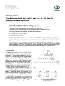
3.1) end for Several comments about the TWIST are in order: (i) Variables with subscript belong to the Landweber iteration . (ii) At Steps 2 and 3.1, is a scaling factor that determines the step size of the Landweber iteration. At Step 3.1, coefficients of the linear combination of and are and with . Here, and are the maximum and minimum singular values of , respectively. (iii) is the thresholding function. For in (8), is termed hard thresholding function [14], and in complex domain if otherwise

end iterations Several comments about the BIM are in order: (i) Variables with superscript belong to the Born iteration . (ii) At Step 2.2, a penalty term, , which is weighted with , is added to the misfit between and to alleviate the ill-posedness of the inverse problem. When , the minimization problem is analytically solved using the Tikhonov method [1]. Also, truncated Landweber or conjugate gradient iterations result in a similar type of regularization scheme [1]. When , , the resulting cost function can be efficiently minimized using IST algorithms (under the assumption that many entries of are zero, i.e., is sparse) [12] (Section II-C). (iii) Born iterations are terminated when the solution converges (Section II-E). (iv) Step 1 uses the first-order Born approximation, i.e., assumes that total field at is same as the incident field. This is used to initialize the iterative algorithm. When is sparse, scattered fields are expected to be weaker and the first-order Born approximation provides a good initial guess for the BIM. As shown by numerical results, this results in faster error convergence at the first few Born iterations independent of the choice of . (v) The system of (3) at Step 2.4 is solved iteratively using the stabilized bi-conjugate gradient (STABICG) method. Since , , , and are Toeplitz, the matrix-vector multiplications required by the STABICG are accelerated using fast Fourier transform (FFT).

, Similarly, for and in complex domain

(9)

is termed soft-thresholding function [14], (10)

Magnitudes of and are plotted in Figs. 1(a) and (b), respectively. The figures reveal that IST, at each iteration, applies a projection-like function to the Landweber iteration, which iteratively imposes the constraint. Thresholding level is determined by the value of (Section II-E). (iv) Landweber iterations are terminated when (Section II-E). Split Augmented Lagrangian Shrinkage Algorithm (SALSA): SALSA makes use of augmented Lagrangian method (ALM) to split the cost function and its argument [15]. Assume that in (8) is split into two variables and , and the cost function is split into and :

Minimizing

under the constraint that and

are equal, (11)

C. Sparse Regularization If it is known priori that the investigation domain is sparse, i.e., many entries of are zero, then the penalty term at Step 2.2 of the BIM is chosen as , , yielding the minimization problems (8) In (8), the first term is a measure of how well the solution fits the noisy data and the second term is a measure of the solution’s regularity. In the remainder of this section, two recently developed IST algorithms, which can be used to efficiently solve the minimization problems in (8), are described. Two-Step IST (TWIST): TWIST is an improved version of the original IST algorithm that incorporates a thresholding shrinkage function

is equivalent to minimizing the cost function in (8). By applying alternating direction method of multipliers (ADMM) [15], (11) is converted into a form where the minimization iteratively alternates between and : Step 1) Step 2) for 2.1) 2.2) 2.3) end for

and ,


3881

permittivity of the embedded crack represents a sparse unknown perturbation to . Let represent the perturbation to at the location of the crack. Assuming the embedding medium completely fills the investigation domain, . Applying the discretization scheme to this equation yields: (12) and Here, (12), Step 2.2 of the BIM is replaced with

,

. Using

(13) while the rest of the BIM iterations is kept unchanged. Note that and are known while is the unknown to be solved for. Then, TWIST and SALSA can be efficiently used within the BIM after is replaced with and is replaced with in the algorithm descriptions. E. Parameter and Stopping Criteria Selection The BIM is terminated when the difference between the solutions at two consecutive iterations becomes small, i.e., when the convergence condition (14) Fig. 1. Thresholding functions on the complex domain for (a) , (soft-thresholding) and (b) , (hard-thresholding).

Here, and are the Lagrange multiplier coefficients associated with the ALM method [15]. Minimization problems at Steps 2.1 and 2.2 are solved analytically using the Tikhonov method and thresholding function , respectively [15]. The resulting SALSA iterations applied at Step 2.2 of the BIM read: and

Step 1) Step 2) for

,

is satisfied. Here, is a user-defined parameter. TWIST and SALSA iterations are truncated by setting a limit on the total number of iterations, i.e., setting . This is done using the following discussion as a guideline. Assume that the convergence condition (14) is satisfied at iteration . Also assume that and are separated into two components: (15) , and . Let Obviously, as represent the noise in , which is defined with respect to scattered field of the original model:

2.1) 2.2) 2.3) end for Several comments about the SALSA are in order: (i) Variables with subscript belong to the SALSA iteration . (ii) Regularization and thresholding parameters and are selected as described in Section II-E. (iii) The system of equations at Step 2.1 is iteratively solved using STABICG. (iv) SALSA iterations are terminated when (Section II-E). D. Sparsification In many inverse EM scattering problems, the targets in the investigation domain are sparse in comparison to a larger scatterer or an embedding medium with known permittivity. Most common examples of these problems are found in the field of non-destructive testing, which typically include crack detection in wood, cement, or paste. For these applications, the permittivity of the embedding medium (wood, cement, or paste) is known. Let and denote this permittivity and the contrast of the embedding medium. Then, the

(16) is the contrast of the original model and is the correwhere sponding matrix computed using (6) with the fields obtained by solving (3) with . Inserting (15) into (16), , an “equivalent” noise figure at iteration is obtained: (17) and . Note that as , , while does not change with . One can think of as the equivalent noise figure at iteration . It has two components: (i) , which represents the measurement error, and (ii) , which is the difference between the scattered field of the original model and the scattered field due to the converged solution of the regularized and linearized model. The discussion here demonstrates that as , gets smaller. Landweber iterations inherent in TWIST, start by recovering the components of the solution associated with the largest singular values and proceed to components associated with smaller ones as the iterations evolve. This means that TWIST iterations should be truncated before they start recovering the components of the solution that are corrupted by the equivalent noise. Therefore, should be set to where

3882


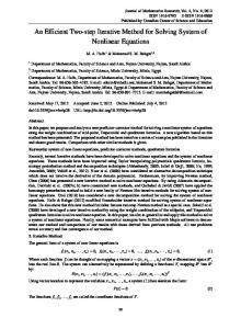
Fig. 3. computed during the execution of the BIM regularized using TWIST, SALSA, and Tikhonov. Fig. 2. Actual permittivity profile and transmitter-receiver locations.

smaller values for small (since the equivalent noise figure is high for small ) and should be increased as . Unlike TWIST, SALSA makes use of Tikhonov inversion. Consequently, at a given SALSA iteration, all components of the solution, which are associated with singular values larger than the regularization parameter , are recovered. Following the discussion above, one could set to higher values for small and decrease it as . But also, it should be realized here that ADMM enforces the equivalency of the minimization problems (8) and (11) iteratively. Obviously, the accuracy of this operation also depends on the maximum number of iterations, . Since the overall accuracy of the Born iterations is lower ( is higher) when is small, is set to a lower value. As , is increased. Under this condition, it is sufficient to set to a fixed value. The thresholding level for both TWIST and SALSA are determined by . This parameter should be chosen in such a way to “remove” the effect of equivalent noise from the solution. Since the effect of varying equivalent noise is taken into account by varying , is set to a fixed value during Born iterations. III. NUMERICAL RESULTS In this section, effectiveness of the IST-BIM in solving 2D inverse EM problems involving sparse and piecewise discontinuous domains is demonstrated via two numerical examples. In these examples, the and is computed using relative norm error between (18) , are generated by adding white Noisy measurement samples, Gaussian noise to the scattered field samples of the original model, and the fields obtained by which are computed using (5) with . The level of noise is measured in decibels (dB) solving (3) with (SNR), where SNR represents the signal to noise ratio. using and , and the level of noise For both experiments, is 25 dB. All simulations were carried out on a Unix workin station with two Intel Xeon X5650, 2.67 GHz processors (12 cores in total) and 48 GB RAM using MATLAB R2012b. A. Austria The relative permittivity profile of the domain, , and the receiver-transmitter configuration are shown in Fig. 2. The 6 m 6 m investigation domain is discretized using square cells with . The sparseness level in is 15%. The dimension numbers of receivers and transmitters are 48 and 12, respectively. The . transmitters are operated at frequency for the BIM iterations regularized using TWIST Fig. 3 plots , , and (i) , , (ii) , with

Fig. 4. Profiles recovered by the BIM regularized using (a) TWIST with and (b) Tikhonov .

, (iii) SALSA with , , and , and (iv) Tikhonov, where the weight of the penalty term is calculated as with . For both TWIST and SALSA for , for , and iterations, , for . The profiles recovered in simulations (i) and (iv) are shown in Fig. 4(a) and (b), respectively. Simulations (i)–(iv) required 60 s, 116 s, 125 s, and 434 s of execution time to reach an error level of 49% in the solution. Note that this is the minimum error level that can be achieved by the Tikhonov-BIM. on the converTo characterize the effect of the parameter gence of the solution, three simulations are carried out: TWIST-BIM for , for , with (i) , for , (ii) for and and , for , and (iii) for all . For all three , , , and and simulations, is plotted in Fig. 5(a). Finally, the effect of the thresholding parameter is characterized via five simulations: TWIST-BIM with and , (ii) , (iii) , and TWIST-BIM (i) and (iv) , (v) . For all five simulawith , , for , for tions, , and , for , and is plotted in Fig. 5(b). B. Pulses Embedded in a Conductive Medium The conductivity profile of the domain and the receiver-transmitter configuration are shown in Fig. 6. The 8.85 m 8.85 m investigation square cells with dimension domain is discretized using . In this example the sparsification method proposed in Section II-D is used. This leads to a sparseness level of 2.7% in . The numbers of receivers and transmitters are both 36. The transmitters . are operated at frequency Fig. 7 plots for the BIM iterations regularized using TWIST , , , and , (ii) , with (i) , , , and (iii) Tikhonov where the weight of


3883

Fig. 8. Conductivity profiles recovered by the BIM regularized using and (b) Tikhonov (a) TWIST with .

C. Comments

Fig. 5. Effects of (a) maximum number of regularization iterations and (b) the thresholding level on the accuracy and convergence of the solution.

Fig. 6. Actual conductivity profile and transmitter-receiver locations.

Several comments about the results presented in Sections III-A and III-B are in order: (i) Convergence in computed for IST-BIM and Tikhonov-BIM is similar (and faster) for the first Born few iterations. This is expected since, for sparse domains, the first-order Born approximation provides a good initial guess for the BIM. For the Tikhonov-BIM, the error gets flat after a certain point indicating that the regularization with second norm penalty term cannot recover the domain with a higher accuracy. On the other hand, IST-BIM maintains the convergence for a higher number of Born iterations (i.e., the error gets flat at a later point and at a lower value). This is expected since it is well known that shrinkage thresholding methods work efficiently up to 30% sparseness levels for signal processing applications [12]. (ii) The profiles recovered by Tikhonov-BIM have artificial wavelike “ripples”. This results in generation of rather noticeable “ghost” scatterers in the domain [Fig. 4(b)]. The IST-BIM eliminates these ripples using thresholding. The resulting images are sharper and more accurate. is faster when soft-thresholding is used. (iii) Convergence in Additionally, for the profile recovered with hard-thresholding, there are few nonzero samples are identified in the background. The latter is due to the use of zero-norm penalty term that promotes a collection of sparse solutions to the minimization problem. Soft-thresholded regularizations result in better constructions since it uses the first-norm as a penalty term. Unlike zero-norm, first-norm penalty term elects only one global solution with enhanced sharp boundaries. (iv) TWIST-BIM with soft-thresholding requires the least amount of execution time for the solution to reach a certain level of accuracy, i.e., it is the most efficient method. (v) Fig. 5(a) demonstrates that the accuracy and convergence of the solution benefits from gradually increasing the as discussed maximum number of regularization iterations, i.e., in Section II-E. (vi) Fig. 5(b) shows that low values of thresholding parameter increases the error in the converged solution. Also, setting a high value for might result in a diverging solution. One can always ) to increase the make a function of (like it is done for convergence in the solution. IV. CONCLUSION

Fig. 7. computed during the execution of the BIM regularized using TWIST and Tikhonov.

the penalty term is calculated as with . The profiles recovered in simulations (i) and (iii) recovered profiles are shown in Figs. 8(a) and (b), respectively. Simulations (i)–(iii) required 64 s, 91 s, and 1401 s, respectively, to reach an error level of 52% in the solution. Note that this is the minimum error level that can be achieved with the Tikhonov-BIM.

Sparsity constraint regularization is used in conjunction with the BIM to solve the 2D inverse EM scattering problem in sparse/sparsified or piecewise discontinuous domains. In the proposed framework, at every BIM iteration, an IST algorithm is used to numerically minimize the zeroth/first-norm regularized cost function. Guidelines for selecting IST regularization parameters are described. Performance of two accelerated IST algorithms, namely, TWIST and SALSA, are studied within the framework of the BIM for solving the 2D inverse EM scattering problem. Indeed numerical experiments demonstrate that IST-BIM produces more accurate solutions than classical Tikhonov-BIM when applied to sparse and piecewise discontinuous domains.

3884


Development of nonlinear inversion schemes with sparsity constraint regularization is underway. The nonlinear schemes will allow accurate imaging in domains with sharp variations, discontinuities, or sparse content even when the contrast is very high.

Parallelization of the Multilevel Fast Multipole Algorithm by Combined Use of OpenMP and VALU Hardware Acceleration Jinbo Liu, Mang He, Kang Zhang, Binbin Wang, and Qingwei Qiu

ACKNOWLEDGMENT The authors would like to thank the King Abdullah University of Science and Technology (KAUST) Supercomputing Laboratory (KSL) for providing the required computational resources.

REFERENCES [1] M. Pastorino, Microwave Imaging. Hoboken, NJ, USA: Wiley, 2010. [2] D. Colton and R. Kress, Inverse Acoustic and Electromagnetic Inverse Acoustic and Electromagnetic Scattering Theory. Berlin: Springer, 2012. [3] R. Zorgati, B. Duchene, D. Lesselier, and F. Pons, “Eddy current testing of anomalies in conductive materials—Part I: Qualitative imaging via diffraction tomography techniques,” IEEE Trans. Magn., vol. 27, no. 6, pp. 4416–4437, 1991. [4] S. D. Rajan and G. V. Frisk, “A comparison between the Born and Rytov approximations for the inverse backscattering,” Geophys., vol. 54, pp. 864–871, 1989. [5] G. Bozza and M. Pastorino, “An inexact Newton-based approach to microwave imaging within the contrast source formulation,” IEEE Trans. Antennas Propag., vol. 57, no. 4, pp. 1122–1132, 2009. [6] W. Chew and Y. Wang, “Reconstruction of two-dimensional permittivity distribution using the distorted Born iterative method,” IEEE Trans. Med. Imag., vol. 9, no. 2, pp. 218–225, 1990. [7] Z. Q. Zhang and Q. H. Liu, “Two nonlinear inverse methods for electromagnetic induction measurements,” IEEE Trans. Geosci. Remote Sens., vol. 39, no. 6, pp. 1331–1339, 2001. [8] Y. Wang and W. Chew, “An iterative solution of the two-dimensional electromagnetic inverse scattering problem,” Int. J. Imaging Syst. Technol., vol. 1, pp. 100–108, 1989. [9] N. Zaiping, Y. Feng, Z. Yanwen, and Z. Yerong, “Variational born iteration method and its applications to hybrid inversion,” IEEE Trans. Geosci. Remote Sens., vol. 38, no. 4, pp. 1709–1715, 2000. [10] A. Abubakar, P. M. Van den Berg, and J. J. Mallorqui, “Imaging of biomedical data using a multiplicative regularized contrast source inversion method,” IEEE Trans. Microw. Theory Tech., vol. 50, no. 7, pp. 1761–1771, 2002. [11] D. W. Winters, B. D. Van Veen, and S. C. Hagness, “A sparsity regularization approach to the electromagnetic inverse scattering problem,” IEEE Trans. Antennas Propag., vol. 58, no. 1, pp. 145–154, 2010. [12] I. Daubechies, M. Defrise, and C. De Mol, “An iterative thresholding algorithm for linear inverse problems with a sparsity constraint,” Commun. Pure Appl. Math., vol. 57, no. 11, pp. 1413–1457, 2004. [13] J. M. Bioucas-Dias and M. A. Figueiredo, “A new TwIST: Two-step iterative shrinkage/thresholding algorithms for image restoration,” IEEE Trans. Image Process., vol. 16, no. 12, pp. 2992–3004, 2007. [14] T. Blumensath and M. E. Davies, “Iterative hard thresholding for compressed sensing,” Appl. Comput. Harmon. Anal., vol. 27, no. 3, pp. 265–274, 2009. [15] M. V. Afonso, J. M. Bioucas-Dias, and M. A. Figueiredo, “Fast image recovery using variable splitting and constrained optimization,” IEEE Trans. Image Process., vol. 19, no. 9, pp. 2345–2356, 2010. [16] H. Bağcı, R. Raich, A. Hero, and E. Michielssen, “Sparsity-regularized Born iterations for electromagnetic inverse scattering,” presented at the IEEE Int. Symp. Antennas and Propagation, San Diego, CA, USA, Jul. 1–5, 2008.

Abstract—A parallel scheme that combines the OpenMP and the vector arithmetic logic unit (VALU) hardware acceleration is presented to speed up the multilevel fast multipole algorithm (MLFMA) on shared-memory computers. Performance of the hybrid parallel OpenMP-VALU MLFMA is investigated and several strategies are employed to improve the overall speedup and parallel efficiency. Effectiveness of the hybrid parallel scheme is verified by numerical results of the electromagnetic (EM) scattering examples, and related numerical stability issue is discussed as well. Index Terms—Electromagnetic scattering, multilevel fast multipole algorithm, OpenMP, parallel computing, vector arithmetic logic unit (VALU).

I. INTRODUCTION As a powerful fast integral equation solver, various parallel schemes of the MLFMA, either based on the single-program-multiple-data (SPMD) [1]–[7] or single-instruction-multiple-data (SIMD) paradigms [8], [9], have been extensively studied. However, in the existing parallelized MLFMA, the vector computing ability provided by modern central processing units (CPUs) was almost neglected [10], [11]. In fact, since Intel Pentium IV, modern CPUs can realize vector computations by virtue of VALU and the instructions of streaming SIMD extensions (SSE). Unlike the floating-point unit (FPU), VALU could simultaneously handle four operands rather than one data sequentially. Therefore, in principle a computer code using VALU could be four times faster than that only uses FPU. This indicates that existing serial or parallel MLFMA codes can benefit from combination of the vector computing capability of VALU through SIMD paradigm and the SPMD parallel model provided by multiple cores of CPU. In contrast to GPU acceleration techniques [8], [9], this hybrid parallel scheme does not require any extra device since VALU is an intrinsic component of CPU; and more importantly, the use of VALU will always enhance the performance of a code, but the same conclusion cannot be applied to the GPU based techniques [10], [11]. In [10] and [11], Yu and Mittra recognized the advantage of VALU in computational electromagnetics for the first time and utilized it with MPI and OpenMP to accelerate their finite-difference time-domain (FDTD) code on a mixed-memory platform. However, it should be pointed out that there are fundamental differences in implementing VALU hardware acceleration with OpenMP to the MLFMA as compared to the FDTD method in shared-memory computers. First, VALU can only operate on pure real operands efficiently, and since all data involved in FDTD method is of real type, it is natural that the FDTD code can make full use of VALU; whereas most numerical calculations in the MLFMA are carried out in complex domain, so the vectorization capability of VALU cannot be directly utilized in the MLFMA if we do not modify the codes appropriately. Moreover, it should be emphasized that existing MLFMA codes may already implicitly use Manuscript received February 02, 2013; revised April 20, 2014; accepted April 28, 2014. Date of publication April 30, 2014; date of current version July 02, 2014. This work was supported by the National Natural Science Foundation of China under Grant 60801008. (Corresponding author: M. He). The authors are with the School of Information and Electronics, Beijing Institute of Technology, Beijing 100081, China (e-mail: [email protected]). Color versions of one or more of the figures in this communication are available online at http://ieeexplore.ieee.org. Digital Object Identifier 10.1109/TAP.2014.2321141

0018-926X © 2014 IEEE. Personal use is permitted, but republication/redistribution requires IEEE permission. See http://www.ieee.org/publications_standards/publications/rights/index.html for more information.