Proceedings of 2005 Particle Accelerator Conference, Knoxville, Tennessee
SIGNAL PROCESSING FOR LONGITUDINAL PARAMETERS OF THE TEVATRON BEAM * S. Pordes#, J. Crisp, B. Fellenz, R. Flora, A. Para, A.V. Tollestrup , FNAL, Illinois 60510, U.S.A. Abstract We describe the system known as the Tevatron SBD [1] which is used to provide information on the longitudinal parameters of coalesced beam bunches in the Tevatron. The system has been upgraded over the past year with a new digitizer and improved software. The quantities provided for each proton and antiproton bunch include the intensity, the longitudinal bunch profile, the timing of the bunch with respect to the low-level RF, the momentum spread and the longitudinal emittance. The system is capable of 2 Hz operation and is run at 1 Hz.
GENERAL DESCRIPTION A schematic is shown in Figure 1. The pick-up is a wide-band resistive wall-current monitor (RWCM) [2] positioned where the proton and antiproton bunches are maximally separated (~200 ns). The signal from the RWCM is brought from the tunnel and digitized in an oscilloscope [3] located in a service building. The scope trigger is provided by the low level RF system. The data are read from the oscilloscope over ethernet and processing is performed in LabView [4] running on a Macintosh G5 computer. Accelerator parameters such as the beam energy and the RF voltage are read from the accelerator control system and the longitudinal quantities are returned via ACNet.
reflections from one channel input will arrive at the other channel with 50 ns (2.5 buckets) delay. The oscilloscope provides 8 bits of resolution. To use this range efficiently, a DC offset in the scope sets the baseline to ~30 counts (out of 255). The high gain channel accomodates the antiproton signal and the proton signal is contained in the low gain channel. In practice, we synthesize the proton signal from both channels thus improving the resolution on the proton signal by ~ 8. The signal is sampled at 5GS/s. To reduce the effect of digitizing noise, a set of 32 sweeps is taken and averaged (within the 6200). Each sweep covers 21 usecs, a full Tevatron period, and successive sweeps are taken every ~ 42 usec, triggered by the Low Level RF proton marker. (The 1.2 millisecond of acquisition is small compared to the synchrotron period of the Tevatron.) A second set of sweeps triggered by the antiproton marker is taken to obtain the antiproton RF timing. The data from an acquisition (200 kbytes) are transferred via ethernet to the Macintosh G5 for processing.
Signal Processing The (gain dependent) time offset between the channels is determined by a simple convolution and linear interpolation is used to align the high gain channel. We have not found any need to correct the gain ratio from its nominal value. A 200 tap (40 ns) FIR filter is applied to remove the effects of dispersion in the long cable [5]. Figure 2 shows a proton bunch with two leading and one trailing`satellites’.The effect of the FIR filter, in particular the removal of the dispersive tail, is evident.
Figure 1: Schematic of SBD
SIGNAL PROCESSING Signal Acquisition The RWCM has broad (>2 GHz) bandwidth with a 1.34 ohm resistance formed by 88 120 ohm resistors across the ceramic gap. We use a Lecroy 6200 oscilloscope as digitizer. The RWCM output is brought to the service building via 280 ft of 7/8” heliax cable and then split to provide two copies of the signal, just upstream of the oscilloscope. The signals are fed to two input channels with a gain ratio of ~8, the present ratio of proton to antiproton intensities. The split is positioned so that any ___________________________________________
*Work supported under DOE contract DE-AC02-76CH03000 #
[email protected]
c 0-7803-8859-3/05/$20.00 2005 IEEE
Figure 2: A proton bunch signal (raw) and after application of the FIR filter. The feature at the far right is a 3/4 % reflection. from one channel through the splitter to the other. Full height of the main bunch is ~5 amps. The baseline is found by a histogramming technique in 18 separate sections as shown in Figure 3.
1362
Proceedings of 2005 Particle Accelerator Conference, Knoxville, Tennessee
proton satellite; it seems that we have a slight overcompensation. The moments (intensity, centroid, rms width, skewness and kurtosis) for each bunch are calculated within windows defined by the region where the appropriate aggregate is positive. The intensity measurement has a resolution of better than 0.5%; the centroid and the rms width measurements have a resolution of about 20 ps. The proton and antiproton bunch centroids under steady state conditions are shown in Figure 5; the shape is believed to be due to beam loading.
Figure 3: Baseline (solid line) around the ring (note the full range of the plot is 0.1 Amps). Aggregate quantities of the beam are derived from an aggregate proton and an aggregate antiproton pulse constructed by summing the 36 sets of signals in the 5 buckets centered on the bucket containing the main bunch. (Linear interpolation is used to compensate for the fact that the sampling clock has a slightly different relationship to the RF buckets for the different bunches). The aggregate proton and antiproton bunches are reproduced below. Note that the peak current varies from 220 amps in the proton bunch to 0.5 amps in proton satellite -2 and from 27 amps in the antiproton bunch to the 0.27 amps peak in the single antiproton satellite.
Figure 5: Centroids of the proton and antiproton bunches. The centroids have proved useful for example in determining instability modes as shown in Figure 6.
Figure 6: Proton centroids during a mode 1 instability; the full scale is +/- 0.2 ns.
Emittance Calculation
Figure 4: The aggregate bunches for protons and antiprotons showing peak currents and the calculated baseline (horizontal white line). The leading satellites suggest an error in the baseline of about 0.05 amps compared to the 220 amp peak of the proton current and 25 amp peak of the antiproton current. The effect of the FIR filter is most evident in the trailing
A new calculation of the beam momentum spread and longitudinal emittance has been implemented. Earlier calculations assuming that the beam is Gaussian in time and momentum spread were in contradiction with the observed time distribution and implied that there was a significant change in the longitudinal emittance between 150 GeV and 980 GeV despite no obvious mechanism for, or symptom of, such a change. A technique [6] that treats any stable phase-space distribution has been developed by A. Tollestrup and implemented in LabVIEW by A. Para. The technique depends on the fact that, for stable beam, the particle density is uniform along an ellipse of constant action in phase space. The procedure starts by dividing the bucket area into a number of constant action ellipses such that the difference in phase space between successive ellipses is the same (Figure 7a). The projection of the
1363
c 0-7803-8859-3/05/$20.00 2005 IEEE
Proceedings of 2005 Particle Accelerator Conference, Knoxville, Tennessee
phase space between successive ellipses on the time (or z) axis is shown in Figure 7b. The SBD time distribution is the sum of these difference projections each multiplied by the beam density for its particular phase space interval. The longitudinal emittance distribution is found by fitting the time distribution to a sum of these projections
Figure 7a: Curves of constant action; the area between successive curves is 10% of the total area.
arbitrary scales involved and the agreement is quite satisfactory except at the time of the beam blow-up.
Figure 9: Comparison of the momentum spread reported by the SBD system and the TeV Schottky.
SUMMARY The Tevatron SBD is now capable of providing reliable values for the longitudinal parameters of the Tevatron beam. The capability of the system has been significantly enhanced with its new digitizer, more sophisticated signal processing and a new algorithm for deriving the momentum spread and longitudinal emittance. There is a small overcompensation in the FIR filter and a small bunch shape dependence in the intensity values which is being worked on.
Figure 7b: projection of the region between successive curves of Fig. 7a. In practice, 25 regions are used. The difference functions are evaluated numerically and the values for beam at 150 GeV and 980 GeV are pre-calculated and stored in the SBD program. Figure 8 shows how the bunch width, momentum spread and emittance change between 150 GeV and 980 GeV.
ACKNOWLEDGEMENTS A. Hahn developed the previous SBD on which this system is based. Little of the work reported here is due to the first author of this paper. F. DeJongh has contributed a useful data viewer. Particular acknowledgement must be made of A.V. Tollestrup who has so stimulated us in this effort and pushed us to our, but not his, limit.
REFERENCES [1] SBD stands for Sampled Bunch Display. [2] B. Fellenz and J. Crisp, BIW 98 An improved Resistive Wall Monitor & AIP Conf. Proceedings 451 pp. 446-453 [3] Lecroy Corporation Waverunner 6200A. [4] LabVIEW - National Instruments Corporation. [5] S. Pordes et al., PAC 2003 Measurement of Proton and Anti-proton Intensities in the Tevatron Collider IEEE Catalog Number 03CH37423C, pp 2491-2493 [6] A.V. Tollestrup, Fermilab Beams Document Data Base (http://beamdocs.fnal.gov/) #541, 548 and 881 [7] R. Pasquinelli et al., PAC2003, A 1.7 GHz Waveguide Schottky Detector System IEEE Catalog Number 03CH37423C, pp 3431-3433
Figure 8:Longitudinal quantities at 150 and 980 GeV. Figure 9 shows a comparison of the momentum spread as determined by the 1.7 GHz TeVatron Schottky [7] with the momentum spread reported by the SBD. There are no
c 0-7803-8859-3/05/$20.00 2005 IEEE
1364