Signature Change, Inflation, and the Cosmological
arXiv:gr-qc/9806109v1 27 Jun 1998
Constant
Reza Mansouri1 and Kourosh Nozari2 Institute for Studies in Theoretical Physics and Mathematics, P.O.Box 19395-5531 Tehran, Iran, and Department of Physics, Sharif University of Technology, P.O.Box 11365-9161, Tehran, Iran. February 5, 2008
Abstract Colombeau’s generalized functions are used to adapt the distributional approach to singular hypersurfaces in general relativity with signature change. Equations governing the dynamics of singular hypersurface is obtained and it is shown that matching leads to de Sitter space for the Lorentzian region. The matching is possible for different sections of the de Sitter hyperboloid. A relation between the radius of S 4 , as the Euclidean manifold, and the cosmological constant leading to inflation after signature change is obtained.
1 2
e-mail: mansouri@netware 2.ipm.ac.ir e-mail:
[email protected]
1
1
Introduction
Hartle and Hawking[1], in constructing a satisfactory model of the universe, try to avoid the initial spacetime singularity predicted by the standard model of cosmology using a combination of general theory of relativity and quantum mechanics. The basic features of the so called “ Hawking Universe” obtained are as follows: 1. A satisfactory theory of quantum gravity will represent the gravitational field, in the manner of general theory of relativity, by a curved spacetime[1]. 2. The proper understanding of ordinary quantum mechanics is provided by Feynman’s “path-integral” or “sum-over-histories” interpretation. In ordinary quantum mechanics the basic idea is that a quantum particle does not follow a single “path” between two spacetime points, and so does not have a single “history”, but rather we must consider all possible “paths” connecting these points. Therefore the usual wave function Ψ is interpreted as an integral over all possible “paths” that a quantum system may take between two state. To solve the path integral, however, one must rotate the time variable in the usual quantum mechanical wave function to imaginary values in the complex plane, which yields as the new time coordinate the “Euclidean” time τ = it [1,2]. 3. There is a wave function for the entire universe ΨU that is given by a Feynman path integral. The basic idea here is that one sums over all possible fourdimensional spacetimes( or spacetime “histories”) connecting two three-dimensional spaces (states). In order to evaluate the path integral, however, one must again rotate the time variable to imaginary values which changes the integral from Lorentzian to Euclidean one. The result is that the temporal variable in the wave function is changed to a spatial one. In other words, ΨU sums only over Euclidean spacetimes, that is, over four-dimensional spaces with positive definite signature (+ + + + )[1-3]. 4. One wants to reach a certain state S at which the evolution of the universe becomes classical, in accordance with general theory of relativity and standard model of cosmology. Accordingly, Hawking proposes a path integral over the Euclidean fourspace gµν , and matter-field configurations φ that yields S. S is characterized by the three-metric hij and a value of the scalar field, φ. 5. To avoid an initial spacetime singularity, the cosmic path integral will include only compact(or closed) four-geometries, so that the three-geometries, marking successive states of the universe, shrink to zero in a smooth, regular way[6]. Hawking’s 2
universal wave function is obtained, therefore, by integrating only over compact four-geometries (Euclidean “spacetimes”) that have the 3-space S as the only (lower) boundary and are such that a universe in state S will subsequently evolve. Statements (3) and (5) above are the essence of the idea that the universe was initially Euclidean and then, by change of signature of “spacetime” metric, the transition to usual Lorentzian spacetime occured. Earlier attempts to describe this interesting aspect was based on Euclidean path integral formulation of quantum gravity and the analogy to quantum tunelling effect in quantum mechanics[1]-[6]. The rise of this idea led many authors to consider it within the classical theory of general relativity[7-20], with some controversies regarding the nature of the energy-momentum tensor of the hypersurface of signature change[15,18,19]. Ellis and his coworkers[8], have shown that classical Einstein field equations, suitably interpreted, allow a change of signature of spacetime. They have also constructed specific examples of such changes in the case of Rabertson-Walker geometries. Ellis[9], by constructing a covariant formalism for signature changing manifolds, has shown the continuity of geodesics over the changing surface. Hayward[10] gives the junction conditions necessary to match a region of Lorentzian-signature spacetime to a region of Riemannian-signature space across a spacelike surface according to the vaccum Einstein or Einstein-Klein-Gordon equations. As we will show, Hayward’s junction condition R˙ = 0 is not compulsory. He has also considered the increasing entropy, large-scale isotropy, and approximate flatness of the universe in the context of signature change[11]. Dereli and Tucker[12], described classical models of gravitation interacting with scalar fields having signature changing solutions. Kossowski and Kriele[13] considered smooth and discontinuous signature change and derived necessary and sufficient junction conditions for both proposals. They investigate the extent to which these are equivalent. They have claimed that non-flat vaccum solutions of Einstein equations can only occur in the case of smooth signature change. Hellaby and Dray[15, 19] argue for a non-vanishing energy-momentum tensor of the signature changing surface. Hayward disagrees to this result and favour a vanishing energy momentum tensor[18]. Kriele and Martin[16] do not accept the usual blief that signature change could be used to avoid space-time singularities, except one abandon the Einstein equations at the signature changing surface. Martin[17] has studied Hamiltonian quantization of general relativity with the change of signature. He has also studied cosmological perturbations on a manifold addmiting signature change. We intend to use the distributional method of Mansouri and Khorrami [21,23] to approach the signature changing problem within the general theory of relativity. This is a powerfull formalism which can also be adapted to our problem, using the Colombeau’s generalized theory of distributions[24-28]. This remedies the difficulties of non-linear operations of 3
distributions in the framework of classical theory of Schwartz Sobolev[29]. In section 2 we give an overview of the Colombeau’s generalized theory of distributions. Sectoin 3 contains the adaptation of the distributional formalism for singular surfaces in general relativity to the case of signature change, followed by concluding remarks in section 4. Conventions and def initions: We use the signature (− + ++) for Lorentzian region and follow the curvature conventions of Misner, Thorne, and Wheeler (MTW). Square brackets, like [F ], are used to indicate the jump of any quantity F at the signature changing hypersurface. As we are going to work with distributional valued tensors, there may be terms in a tensor quantity F proportional to some δ-function. These terms are denoted by Fˆ .
2
A short review of Colombeau theory
Classical theory of distributions, based on Schwartz-Sobolev theory of distributions, doesn’t allow non-linear operations of distributions [29]. In Colombeau theory a mathematically consistent way of multiplying distributions is proposed. Colombeau’s motivation is the inconsistency in multiplication and differentiation of distributions. Take, as it is given in the classical theory of distributions, θn = θ
∀ n = 2, 3, . . . ,
(1)
where θ is the Heaviside step function. Differentation of (1) gives, nθn−1 θ′ = θ′ .
(2)
2θθ′ = θ′ .
(3)
2θ2 θ′ = θθ′ .
(4)
Taking n = 2 we obtain Multiplication by θ gives, Using (2) it follows
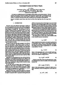
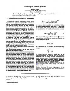
2 ′ 1 ′ θ = θ, (5) 3 2 which is unacceptable because of θ′ 6= 0 . The trouble arises at the origin being the unique singular point of θ and θ′ . If one accepts to consider θn 6= θ for n = 2, 3, . . ., the inconsistency can be removed. The difference θn − θ , being infinitesimal, is the essence of Colombeau theory of generalized functions. Colombeau considers θ(t) as a function with “microscopic structure” at t = 0 making θ not to be a sharp step function ( Fig.1), but having a width τ [24]. θ(t) can cross the normal axis at any value ǫ where we have chosen 4
it to be ǫ > 12 [29]. It is interesting to note that the behaviour of θ(t)n around t = 0 is not the same as θ(t)(Fig.2), i.e. θ(t)n 6= θ(t) around t = 0[24]. In the following we give a short formulation of Colombeau’s theory. Suppose Φ ∈ D(IRn ) with D(IRn ) the space of smooth(i.e.C ∞ ) C-valued test functions on IRn with compact support and Z Φ(x)dx = 1. (6) For ǫ > 0 we define the rescaled function Φǫ (x) as Φǫ (x) =
1 x Φ( ). ǫn ǫ
(7)
Now, for f : IRn −→ C, not necessarily continuous, we define the smoothing process for f as one of the convolutions ˜ := f(x)
Z
f (y)Φ(y − x)dn y,
(8)
f˜ǫ (x) :=
Z
f (y)Φǫ (y − x)dn y.
(9)
or
According to (7), equation (9) has the following explicit form f˜ǫ (x) :=
Z
f (y)
1 y−x n Φ( )d y. ǫn ǫ
(10)
This smoothing procedure is valid for distributions too. Take the distribution R , then by smoothing of R we mean one of the two convolutions (8) or (9) with f replaced by R . Remember that R is a C-valued functional such that Φ ∈ D(IRn ) =⇒ (R, Φ) ∈ C,
(11)
where (R, Φ) is the convolution of R and Φ. Now we can perform the product Rf of the distribution R with the discontinuous function f through the action of the product on a test function Ψ. First we define the product ˜ ǫ with f˜ǫ and then take the limit of corresponding smoothed quantities R (Rf, Ψ) = lim ǫ→0
Z
˜ ǫ (x)f˜ǫ (x)Ψ(x)dn x. R
(12)
The multiplication so defined does not coincide with the ordinary multiplication even for continuous functions. Colombeau’s strategy to resolve this defficulty is as follows. Consider one-parameter families (fǫ ) of C ∞ functions used to construct the algebra EM (IR n ) = {(fǫ ) | fǫ ∈ C ∞ (IRn ) ∀K ⊂ IRn compact, ∀α ∈ IN n ∃N ∈ IN , ∃η > 0, ∃c > 0 such that supx∈K |D α fǫ (x)| ≤ cǫ−N ∀0 < ǫ < η}, 5
(13)
where
∂ |α| D = , (∂x1 )α1 · · · (∂xn )αn α
(14)
and |α| = α1 + α2 + · · · + αn . Accordingly, C ∞ -functions are embedded into EM(IR n ) as constant sequences. For continuous functions and distributions we require a smoothing kernel φ(x), such that Z
Z
dn x ϕ(x) dx = 1 and
dn x xα ϕ(x) = 0 |α| ≥ 1.
(15)
Smoothing is defined as (10) for any function f . Now, we have to identify different embeddings of C ∞ functions. Take a suitable ideal N (IRn ) defined as N (IR n ) = {(fǫ ) | (fǫ ) ∈ EM (IR n ) ∀K ⊂ IR n compact, ∀α ∈ IN n , ∀N ∈ IN ∃ η > 0 , ∃ c > 0 , such that supx∈K |D α fǫ (x)| ≤ c ∈N ∀0 < ǫ < η},
(16)
containing negligible functions such as f (x) −
Z
dn y
1 y−x ϕ( )f (y). ǫn ǫ
(17)
Now, the Colombeau algebra G(IRn ) is defined as, G(IR n ) =
EM(IR n ) N (IR n )
(18)
A Colombeau generalized function is thus a moderate family (fǫ (x)) of C ∞ functions modulo negligible families. Two Colombeau objects (fǫ ) and (gǫ ) are said to be associate (written as (gǫ ) ≈ (fǫ )) if limǫ→0
R
dn x (fǫ (x) − gǫ (x)) ϕ(x) = 0 ∀ ϕ ∈ D(IRn ).
(19)
For example, if ϕ(x) = ϕ(−x) then δθ ≈ 12 δ, where δ is Dirac delta function and θ is Heaviside Step function. Moreover, we have in this algebra θn ≈ θ and not θn = θ. For an extensive introduction to Colombeau theory, see[24,25].
6
3
Distributional Approach to Signature Change
There are two methods of handling singular hypersufaces in general relativity. The mostly used method of Darmois-Israel, based on the Gauss-Kodazzi decomposition of space-time, is handicapped through the junction conditions which make the formalism unhandy. For our purposes the distributional approach of Mansouri and Khorrami (M-Kh) [23] is the most suitable one. In this formalism the whole space time, including the singular hypersurface, is treated with a unified metric without bothering about the junction conditions along the hypersurface. These conditions are shown to be automatically fulfilled as part of the field equations. In the M-Kh-distributional approach one choose special coordinates which are continuous along the singular hypersuface to avoid non-linear operations of distributiuons. Here, using Colombeau algebra, which allows for non-linear operations of distributions, we generalize the M-Kh method to the special case of signature changing cosmological models. Consider a spacetime with the following FRW metric containing a steplike lapse function ds2 = −f (t)dt2 + a2 (t)(
dr 2 + r 2 dθ2 + r 2 sin2 θdϕ2 ), 1 − kr 2
(20)
where f (t) = θ(t) − θ(−t).
(21)
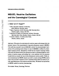
It describes a signature changing spacetime with the singular surface t = 0. The metric describes a Riemanian space for t < 0 and a Lorenzian space-time for t > 0. As has been argued before f (t), analogous to θ(t), has a microscopic structure around t = 0 with a jump equal to τ as shown in Fig.3. We choose again 1 with ǫ > . 2
θ(t) |t=0 = ǫ
(22)
Since θ(−t) = 1 − θ(t), we have θ(−t) = 1 − ǫ and f (t) = 2ǫ − 1.
(23)
This value gives us the correct change of sign in going from t < 0 to t > 0. This “regularization” of f (t) at t = 0 allows us to use operations such as f (t)−1 , f (t)2 , and |f (t)|−1. The physical interpretation of this behaviour of f (t) is that the phenomenon of signature change occurs as a quantum mechanical tunneling effect. This tunneling occurs in a width equal to the width of the jump, i.e. τ . In what follows we consider f (t) to be the regularized function f˜ǫ , defined according to Colombeau’s algebra. Now, we are prepared to calculate the dynamics of the signature changing hypersurface in the line of M-Kh procedure[23]. First we calculte the relevant 7
components of the Einstein tensor, Gtt and Grr , for the metric (20): 1 n 3 −2¨ 3 2af a af + f˙a˙ af + f˙a˙ ¨ − af˙a˙ + 4(kf 2 + f a˙ 2 ) o 3 −2¨ + f − , Gtt = − 2 fa 2 2 f 2a 2 a2 f 2
(24)
and Grr = − 21
2a¨ af −af˙a+4f ˙ a˙ 2 +4kf 2 f 2 (1−kr 2 )
−
1 a2 2 1−kr 2
n
af +a˙ f˙ 3 −2¨ 2 f 2a
−
o 2 +f a af −af˙a+4(kf ˙ ˙ 2) 3 2a¨ 2 2 2 R f
(25)
According to standard calculus of distributions, we have ˙ − θ(−t) ˙ f˙(t) = θ(t) = δ(t) + δ(−t) = 2 δ(t),
(26)
taking into account δ(−t) = δ(t) . Now, using Colombeau algebra we can write 1 θ(t)δ(t) ≈ δ(t). 2
(27)
f (t) δ(t) = θ(t)δ(t) − θ(−t)δ(t) ≈ 12 δ(t) − 12 δ(t) ≈ 0,
(28)
Therefore we may write
In evaluating (24, 25) we should take care of the following property of association. Having AB ≈ AC, we are not allowed to conclued B ≈ C. Now, using the relations (27) and (28) we obtain for the singular parts of equations (24) and (25) ˆ tt = 0, G (29) 2aa˙ ˆ rr = − G δ(t). (30) f 2 (1 − kr 2 ) where multiplication of the distribution δ(t) with the discontinuous functions f12 is defined as in (12). According to [23] the complete energy-momentum tensor can be written as + − Tµν = θ(t) Tµν + θ(−t) Tµν + CSµν δ(t),
(31)
± where Tµν are energy-momentum tensors corresponding to Euclidean and Lorentzian regions respectively and C is a constant which can be obtain by taking the following pill-box integration defining Sµν [23]:
Sµν = lim
Σ→0
1 Λ (Tµν − gµν )dn = lim κ κ Σ→0 −Σ
Z
Σ
8
Z
Σ
−Σ
Gµν dn,
(32)
Since Tˆµν = CSµν δ(Φ(x)), and
Z
Tˆµν dn = CSµν
Z
δ(Φ(x))dn = CSµν |
(33) dn |, dΦ
(34)
we find
dΦ | = |nµ ∂µ Φ|, (35) dn where Φ = t = 0 defines the singular surface Σ. The vector nµ is normal to the surface Φ and n measure the distance along it. Using the metric (20) we obtain C=|
C=
1 . |f (t)|
(36)
The distributional part of the Einstein equation reads as follows: ˆ µν = κTˆµν . G
(37)
we obtain using equations (29,30,33,36,37): 0= and −
κ Stt δ(t), |f (t)|
κ 2aa˙ δ(t) = Srr δ(t). 2 − kr ) |f (t)|
f 2 (1
(38)
(39)
Now using equation (12), we must define the multiplication of δ-distribution with the discontinuous functions |f1| and f12 . To this end we consider them as Colombeau’s regularized functions, ˜ 1ǫ (t) = δǫ (t)( 1 ) (40) G |f (t)| ǫ and
˜ 2ǫ (t) = δǫ (t)( 1 ) . G f 2 (t) ǫ
(41)
Now according to (12), these two multiplications are as follows, 1 , Ψ) = lim ǫ→0 |f (t)|
Z
˜ 1ǫ(t) Ψ(t)dt G
(42)
1 (δ(t) 2 , Ψ) = lim ǫ→0 f (t)
Z
˜ 2ǫ(t) Ψ(t)dt G
(43)
(δ(t) and
˜ 1ǫ and G ˜ 2ǫ are associate in Colombeau’s for any test function, Ψ. Now we argue that G sense, i.e. Z ˜ 1ǫ (t) − G ˜ 2ǫ (t))Ψ(t)dt = 0. (44) lim (G ǫ→0
9
˜ 1ǫ and G ˜ 2ǫ are divergent at a common point, the difThis is correct because although G ference in their “ microscopic structure” at that point tends to zero for ǫ → 0. Therefore, we obtain from (38), (39), and (44) the final form of the energy-momentum tensor of the singular surface, or the dynamics of, Σ: Stt = 0, and Srr = −
2aa˙ . κ(1 − kr 2 )
(45)
(46)
If, along the above line, we compute the Sθθ and Sφφ we find, Sθθ =
−2r 2 aa˙ , κ
(47)
and
−2r 2 sin2 θaa˙ . (48) κ Taking the metric (20) and the results (45-48) we obtain for the so-called ’energy-momentum’ tensor of the singular hypersurface Sφφ =
κSµν = diag(0, −2H, −2H, −2H), where, as usual, we have chosen
(49)
a˙ H= . a
(50)
a = a◦ eHt ,
(51)
Integrating this equation, gives which shows de Sitter expansion of scale factor corresponding to the inflationary phase after signature change. This is in accordance with the features of the so-called “Hawking Universe”[1].
4
Junction conditions and interpretation of the results
Take the metric (20) with a defined as in (50, 51): ds2 = ∓dt2 + e2Ht (dx2 + dy 2 + dz 2 ).
(52)
These coordinates cover half of the de Sitter Hyperboloid for −∞ < t < +∞(30). The hypersurfaces t = t0 are spacelike, except for t = −∞ which is null and the boundary of coordinate patch. 10
The Euclidean section can be interpreted as a S 4 with radius R = H −1 [1]. In the Lorentzian section we are faced with an exponentially expanding universe in which the Hubble parameter is the constant H = aa˙ , irrespective of signature changing time t0 . The cosmological constant in the Lorentzian sector is Λ = 3H 2 , where Therefore, there is the following relation between the cosmological constant and the radius of S 4 : Λ=
3 R2
(53)
Now, the boundary of the Euclidean part is defined by T = constant. These sections are S 3 having a radius equal to a = exp HT . If the matching is along a section corresponding to less (more) than a hemisphere then the radius a of S 3 will increase (decrease) with T [1]. Hence, the expansion in Lorenzian part, i.e. a˙ > 0, means that the matching corresponds to a part of S 4 which is less than a hemisphere where the radius of the boundary increases with the coordinate T . We now go on to calculate the extrinsic curvatures to check the junction conditions [23]. In the Lorentzian region the non-vanishing components of affine connection are Γ011 = Γ022 = Γ033 = He2Ht .
(54)
The extrinsic curvature is defined as [23] Kij = eµi eνj ∇µ nν ,
(55)
where ei , the mutualy normal unit 4-vectors in signature changing surface Φ, are defined as ∂xµ , i = 1, 2, 3. eµi = ∂ξ i ξ i are coordinates adopted to the signature changing surface Σ. ∇µ shows the covariant derivative with respect to the 4-geometry. We then find for the non-vanishing component of extrinsic curvature − − − K11 = K22 = K33 = He2Ht , (56) or K1− 1 = K2− 2 = K3− 3 = H
f or t > −∞,
(57)
K1− 1 = K2− 2 = K3− 3 = 0 f or t = −∞.
(58)
and Similarly, if we consider plus sign in (52), we find for the Euclidean embedding K1+ 1 = K2+ 2 = K3+ 3 = −H,
11
(59)
independent of t being 0 < t < π. The jump in the extrinsic curvature is thus [Kij ] ≡ Ki− j − Ki+ j = 2H,
f or t > −∞,
(60)
and [Kij ] = H,
f or t = −∞.
(61)
Now, the junction condition for the matching is [23] κSij = [Kij ] − hji [K]
(62)
Comparing (60,61) we see that the matching condition is satisfied only for t = −∞. We therefore conclude that for these coordinates chosen for the de Sitter space the matching to a Euclidean space is possible only for the section of space representing t = −∞, which is a null hypersurface.
5
Matching in a different coordinates
The previous section shows that the requirement of signature change leads us to the de Sitter space in the Lorenzian part of the manifold and S 4 in the Euclidean part. This is in agreement with the results of quantum cosmology and minisuperspace considerations[1]. It is however well known that different coordinates for de Sitter space corresponds to different t = constant sections. The above de Sitter coordinates, for example, which cover only half of the de Sitter hyperboloid, are equivalent to k = 0 flat three space sections[30]. Now, there is another useful coordinates familiar from Robertson-Walker metrics which cover the entire de Sitter hyperboloid and its t = constant sections are surfaces of constant q 3 curvature k = 1. These S spaces have a minimum radius equal to Λ3 . We will now try the matching along these sections of de Sitter space. Consider the following metric with approprtiate lapse function corresponding to signature change[30] ds2 = −f (t)dt2 + α2 cosh2 (α−1 t)(dχ2 + sin2 χ(dθ2 + sin2 θdφ2 ))
(63)
where f (t) is defined as in (21). Following the same procedure as for (20) and again using Colombeau’s algebra, we fined for elements of energy-momentum tensor of the hypersurface 2 2 2 (64) κSµν = diag(0, − tanh(α−1 t), − tanh(α−1t), − tanh(α−1 t)), α α α The hypersurface of signature change is defined as t = t0 . The non-vanishing compopnents of the extrinsic curvature are 1 Ki− i = − tanh(α−1t0 ) i = 1, 2, 3. (65) α 12
The corresponding components in the Euclidean embedding are Ki− i =
1 tanh(α−1 T0 ), α
(66)
where we have used a different symbol T as the coordinate in the Euclidean region corresponding to ’time’. This is allowed because the hypersurface of signature change as the boundary of the two different manifolds is defined differently in each of them. Now the jump of extrinsic curvature on the signature change surface is 1 1 [Kii ] ≡ Ki− i − Ki+ i = − tanh(α−1 t0 ) − tanh(α−1 T0 ). α α
(67)
Now the junction condition (62) is satisfied for t0 = T0 = 0. Therefore, the matching is q 3 done along the section of de Sitter space with the minimum radius Λ , which is equal to the radius of corresponding section of the Euclidean manifold.
6
conclusion
As we have seen in the previous sections signature change is only possible for de Sitter space in the Lorenzian part of the manifold. Depending of the coordinate patches one use on the de Sitter hyperboloid, different matchings are possible. Using de Sitter coordinates which cover only half of the hyperboloid the matching is along the t = −∞ which is a null hypersyrface. For the Robertson-Walker type metric covering the entire hyperboloid the matching is along the hypersurface of minimum radius of the de Sitter hyperboloid. In both cases the cosmological constant is given by the radius of the Euclidean S 4 . We have therefore a geometrical interpretation for the value of the cosmological constant. Vanishing of the cosmological constant would mean that the Euclidean manifold is an R4 which is noncompact and therefore contradicts the quantum cosmological considerartions. Now, it is very reasonable to take for the radius of S 4 the only fundamental length q that we have, namely the Planck length. We therefore come to the conclusion that lP l = Λ3 .
References [1] J. B. Hartle and S. W. Hawking, Phys. Rev. D 28 (1983) 2960 and S. W. Hawking, Nucl. Phys. B 239 (1984) 257 [2] J. J. Halliwell and J. B. Hartle, Phys. Rev. D 41 (1990) 1815 [3] G. W. Gibbons and J. B. Hartle, Phys. Rev. D 42 (1990) 2458 [4] C. J. Isham, Class. Quantum Grav. 6 (1989) 1509 13
[5] G. T. Horowitz, Class. Quantum Grav. 8 (1991) 587 [6] G. W. Gibbons and S. W. Hawking, Commun. Math. Phys. 148 (1992) 345 [7] A. D. Sakharov, Sov. Phys. JETP 60 (1984) 214 and see also B. L. Al’tshuler and A. O. Barvinsky, Phys. Uspekhi 39 (5) (1996) 429 [8] G. F. R. Ellis, A. Sumruk, D. Coule and C. Hellaby, Class. Quantumm Grav. 9 (1992) 1535 [9] G. F. R. Ellis, Gen. Rel. Grav. 24 (1992) 1047 [10] S. A. Hayward, Class. Quantum Grav. 9 (1992) 1851 [11] S. A. Hayward, Class. Quantum Grav. 10 (1993) L7 [12] T. Dereli and R. W. Tucker, Class. quantum Grav. 10 (1993) 365 [13] M. Kossowski and M. Kriele, Class. Quantum Grav. 10 (1993) 1157 ; M. Kossowski and M. Kriele, Class. Quantum Grav. 10 (1993) 2363 [14] S. A. Hayward, Class. Quantum Grav. 11 (1994) L87 [15] C. Hellaby and T. Dray, Phys. Rev. D49 (1994) 5096 [16] M. Kriele and J. Martin, Class. Quantum Grav. 12 (1995) 503 [17] J. Martin, Phys. Rev. D 49 (1994) 5086 ; J. Martin, Phys. Rev. D 52 (1995) 6708 [18] S. A. Hayward, Phys. Rev. D 52 (1995) 7331 [19] C. Hellaby and T. Dray, Phys. Rev. D 52 (1995) 7333 [20] T. Dray, C. A. Manogue and R. W. Tucker, Gen. Rel. Grav. 23 (1991) 967 ; T. Dray, C. a. Manogue and R. W. Tucker, Phys. Rev. D 48 (1993) 2587 ; T. Dereli, M. ¨ Onder and R. Tucker, Class. Quantum Grav. 10 (1993) 1425 ; I. L. Egusquiza, Class. Quantum Grav. 12 (1995) L89 ; M. D. Maia and E. M. Monte, gr-qc/9501031 ; S. A. Hayward, gr-qc/9502001 ; L. J. Alty and C. J. Fewster, gr-qc/9501026 ; T. Dray, C. A. Manogue and R. W. Tucker, gr-qc/9501034 ; M. Kriele, gr-qc/9610016 ; T. Dray, J. Math. Phys. 37 (11) (1996) 5627 ; B. Z. Iliev, gr-qc/9802057 and gr-qc/9802058 [21] M. Khorrami and R. Mansouri, J. Math. Phys. 35 (1994) 951 [22] D. Hartly and coworkers, gr-qc/9701046 and T. Dray, gr-qc/9701047 [23] R.Mansouri and M. Khorrami, J. Math. Phys. 37 (11) (1996) 5672 14
[24] J. F. Colombeau, Multiplication of Distributions, LNM 1532, Springer (1992) [25] M. Oberguggenberger, Multiplication of Distributions and Aplications to PDEs, Longman, 259 (1992) [26] H. Balasin, gr-qc/9610017 [27] C. Clark, J. Vickers and J. Wilson, Class. Quantum Grav. 13 (1996) 2485 [28] J. Wilson. gr-qc/9705032 [29] R. M. Kanwal, Generalizsd Functions: Theory and Technique, Academic press, 1983 [30] S. W. Hawking and G. F. R. Ellis, The Large Scale Structure of Spacetime, Cambridge University Press, 1973
15