edges of a triangle mesh, the surface is not C1 continuous, hence .... the intersections of a ray going from the given point to infinity .... the face case there is one incident face, namely the face ... On the left, x is .... unnormalized convex hull normal, nh, is then found as .... where multiple distances are computed, it is possible to.
ENGLISH XX
1
Signed Distance Computation using the Angle Weighted Pseudo-normal J. Andreas Bærentzen and Henrik Aanæs, Member, IEEE
Abstract— The normals of closed, smooth surfaces have long been used to determine whether a point is inside or outside such a surface. It is tempting also to use this method for polyhedra represented as triangle meshes. Unfortunately, this is not possible since at the vertices and edges of a triangle mesh, the surface is not C 1 continuous, hence, the normal is undefined at these loci. In this paper, we undertake to show that the angle ¨ weighted pseudo-normal (originally proposed by Thurmer ¨ and Wuthrich and independently by Sequin) has the important property that it allows us to discriminate between points that are inside and points that are outside a mesh, regardless of whether a mesh vertex, edge or face is the closest feature. This inside-outside information is usually represented as the sign in the signed distance to the mesh. In effect, our result shows that this sign can be computed as an integral part of the distance computation. Moreover, it provides an additional argument in favour of the angle weighted pseudo-normals being the natural extension of the face normals. Apart from the theoretical results, we also propose a simple and efficient algorithm for computing the signed distance to a closed C 0 mesh. Experiments indicate that the sign computation overhead when running this algorithm is almost negligible. Index Terms— mesh, signed distance field, normal, pseudo-normal, polyhedron.
I. I NTRODUCTION
T
HE far most popular way of representing 3D objects in computers is as triangle meshes. Often, these triangle meshes are closed, thus representing polyhedra. When dealing with such 3D objects, it is often crucial to be able to determine how they relate to each other. In particular, we may want to know whether two objects interpenetrate or whether a given path collides with an object. A fundamental prerequisite for such queries is the ability to determine whether a given point in space Received: XXX J.A.Bærentzen and H. Aanæs are both with the Informatics and Mathematical Modelling Department of the Technical University of Denmark, DK-2800 Kongens Lyngby, Denmark. E-mail: {jab, haa}@imm.dtu.dk
is inside or outside a 3D object—here assumed to be a triangle mesh. For objects with closed, smooth, and orientable surfaces, the surface normal is an important tool for determining whether a given point is inside or not. This is done by finding a point, c, on the surface and taking the inner product of the surface normal at c with the vector between the given point p and c, i.e. r = p−c. However, an object represented as a polyhedron or mesh is not a smooth surface, and, hence, does not have normals defined everywhere on the surface (i.e. the surface is discontinuous at edges and vertices). At the outset, the above simple scheme is therefore not deemed possible. It is, however, possible to define vectors at edges and vertices which posses some of the properties of normals, and these we denote pseudo-normals. Naturally, there is a variety of these pseudo-normals capturing different properties of normals. In the case of determining whether a point is inside a polyhedron, it turns out that the angle weighted pseudo-normal proposed by Th¨urmer and W¨uthrich [1] and independently by Sequin [2] captures the necessary properties. Thus, the above mentioned simple scheme can be used for polyhedra as well. To our knowledge, this has not been observed before. The main contribution of this paper is proposing and proving that the angle weighted pseudo-normal can be used for determining whether a point is inside a polyhedron. Specifically, we show that the sign of the inner product between the angle weighted pseudo-normal and the vector to an arbitrary point from its closest point on the surface uniquely determines whether that given point is inside the polyhedron or not. In addition, we argue that this is a rather unique property of the angle weighted pseudo-normal, in that all other proposed analytic pseudo-normals, we have been able to find, do not possess this property. Hence, valuable insight into the geometry of the widely used polyhedron or mesh based object structures is provided. Finally, we argue that the proposed procedure for determining whether a point is inside or outside is also numerically robust. In order to demonstrate the applicability of this result, it is used to propose a scheme for signed distance to triangle mesh computation. In essence this scheme
ENGLISH XX
consists of extending any unsigned distance algorithm to calculate the signed distance as well. Fortunately, all unsigned distance algorithms find the closest point on the mesh, c, to all considered points, p. In conjunction with the angle weighted pseudo-normal this is enough information to compute the sign. We propose an efficient algorithm for computing the signed distance to a mesh from a point in a general position. The algorithm is similar in structure to other algorithms for computing the unsigned distance [3], [4]. The algorithm requires a hierarchical representation of the mesh, and our results show that once this hierarchy has been built, the overhead incurred by computing the sign is negligible compared to the distance computation. The performance of our method is measured by generating 3D grids of signed distances for a number of models, and we compare the performance to a method for computing only the sign. Signed distances are important for a number of applications. For instance, signed distance fields (i.e. grids of voxels holding distances) are often used to initialize the level set method [5], [6] which, in turn, has many applications in e.g. computer vision and computer graphics [7]. Although beyond the scope of this paper, we envision that the result also has relevance for other applications, most notably path planning, offset surfaces, and collision detection, c.f. [8], [9] all of which can be approached via signed distances or signed distance fields [10]. A. Overview and Relations to Other Work The main result of this paper is the proof that the angle weighted pseudo-normal can discriminate between points that are inside and points that are outside a triangle mesh or polyhedron1 . The angle weighted pseudonormal is discussed in detail in Section II, and the proof is found in Section III. Other solutions have been proposed for addressing the point in polyhedron problem. The best known is counting the intersections of a ray going from the given point to infinity, since the number of intersections must be odd if the point is inside. A robust way to implement this procedure is due to Linhart [11]. Another scheme based on testing the inclusion of the point in tetrahedra formed between each face and the origin was proposed by Feito et al [12]. Finally, a different method based on summing the area of spherical polygons was proposed in [13] by Carvalho et al. For earlier work see also references in [11] and [12]. In general, the previous methods must visit the entire mesh and their run time is at best linear 1
In the following we will use the two terms interchangeably.
2
in the number of faces. This is certainly true of [12], [13]. Using intersection counting [11], we only need to visit the parts of the mesh that are pierced by a ray going from the given point to infinity. However, our method only needs to find the closest point on the mesh, which can be even faster. Our primary application for the work in this paper is the generation of discrete signed distance fields from triangle meshes. There is a good deal of literature on this topic, and in the following we review the most relevant papers. Payne and Toga [3] discuss many issues pertaining to distance fields. One of these is the generation of distance fields from triangle meshes, optimizations, and the correct computation of signs. Payne and Toga addressed the sign problem by suggesting that the mesh is scan converted separately. Jones [14] also uses scan conversion and computes the distance for voxels only in the vicinity of sign changes. Dachille et al. [15] proposed a method for computing the distance to a triangle using only incremental plane calculations. Their technique is amenable to hardware implementation. Mauch proposed a novel scan conversion method [16]. The idea is to generate a so called characteristic for each mesh feature (i.e. each edge, vertex, and face). A characteristic is essentially the Voronoi neighborhood of the feature. All voxels inside the same characteristic are closest to the same feature. Sigg et al. extended Mauch’s method in [17]. In order to make the method sufficiently fast when the final scan conversion is performed on graphics hardware, they reduced the number of characteristics producing only one for each triangle. Another hardware accelerated method for generating distance fields was proposed recently by Sud et al. in [18]. Occlusion queries are used to cull away features that cannot contribute to the distance field, and the maximum extent of the contribution of a feature is bounded using observations regarding spatial coherence. This paper extends unsigned distance algorithms to include sign. If such an algorithm is used to compute signed distance fields, this implies that, unlike in all of the above methods, there is no need for scan conversion [19]. Although scan conversion is not intrinsically difficult there are some pitfalls mentioned in Section V. The algorithm for signed distance computation is discussed in Section IV. Some authors have investigated alternative distance field representations where distances are not stored in a regular voxel grid. For instance, Frisken et al. proposed the use of adaptive distance fields [20]. Huang et al. suggested the notion of complete distance fields [21] where information about the initial triangles is kept
ENGLISH XX
3
in a 3D grid. Gueziec [4] used a hierarchical mesh PSfrag representation to quickly compute distances. His method is especially efficient if the mesh deforms. The work by Gueziec extended ealier work in collision detection by Johnson et al. [22] and Larsen et al. [23]. Recently, Wu et al. pursued a similar strategy [24]. They generate a BSP tree, c.f. [25], where each node contains a linear approximation of the distance field. The distance field is only C −1 but of bounded error. While a detailed discussion of the methods above is beyond our scope, they are mentioned, in part, because it is likely that they could benefit from the proposed sign computation scheme. As mentioned, several pseudo-normals have been proposed. Probably the earliest is due to Gouraud who suggested using the (unweighted) sum of face normals as a vertex normal [26]. Th¨urmer et al. [1] and Sequin [2] independently proposed the sum of angle weighted face normals, and Glassner and Max have proposed yet other ways to compute normals [27], [28]. These techniques are discussed in detail in Section II-A. Lastly, a previous and less complete publication of this work is [29]. II. A NGLE W EIGHTED
PSEUDO - NORMAL
First some formalism. Let M denote a triangle mesh. Assume that M describes a closed, orientable 2– manifold in 3D Euclidean space, i.e. the signed distance problem is well defined. Denote by M the closure of the interior of M , i.e. M = ∂M. Define the unsigned distance from a point p to M as2 d(p, M ) = inf kp − xk ,
(1)
x
replacements α1 α2 Fig. 1.
2
Infimum is the greatest lower bound of a set, denoted inf.
The incident angels {α1 , α2 , α3 , . . . } of point x ∈ M .
a line segment defined by the normal, it is clear that kp − ck if p outside surface −kp − ck if p inside surface , n · (p − c) = 0 if p on surface (2) In the case of piecewise planar surfaces, M , the Voronoi regions form line segments only if c belongs to a face. If c belongs to an edge, V (c) is a wedge delimited by the face normals. In the case of a vertex, V (c) is a cone whose apex coincides with c. The edges of the cone are defined by the face normals. Unfortunately, this means that (2) no longer holds if the point c belongs to an edge or a vertex. Hence, an obvious question is whether we can formulate a pseudo– normal for any locus c on a mesh such that a modified form of (2) holds. The main contribution of this paper is proving that for the angle weighted pseudo–normal, nα the following holds nα · (p − c) > 0 if p outside surface nα · (p − c) < 0 if p inside surface . nα · (p − c) = 0 if p on surface
(3)
The angle weighted pseudo–normal is defined as follows: For a given face, denote the normal3 as n, which is assumed pointing outward. I.e., if the closest point, c ∈ M , to p is on a face, then the sign is given by
x∈M
and let the sign be determined by whether p is in M, positive denoting p ∈ / M. The optimum or optima in (1) are the closest point(s) to p. We use c to denote a closest point. Conversely, for a given point c on the mesh, there is a set of points V (c) such that for p ∈ V (c), c is the surface point closest to p. The set V (c) is the Voronoi region of c. For a solid with a differentiable surface, the Voronoi regions form line segments from c in the positive and negative directions of the normal n at c. These line segments are either semi-infinite or terminate at points of equal distance to two surface points (i.e. points on the medial axis). Since any p ∈ V (c) lies on
α3
sign (r · n) ,
r=p−c .
(4)
The angle weighted pseudo-normal for a given point, x ∈ M is then defined as P αi n i , (5) nα = Pi || i αi ni || where i runs over the faces incident with x and αi is the incident angle, c.f. Figure 1. Even though Th¨urmer and W¨uthrich [1] only considered this angle weighted pseudo-normal for vertices of the mesh, it generalizes nicely to faces and edges. In the face case there is one incident face, namely the face itself, hence 2πn1 n1 = n α = , ||2πn1 || 3
It is assumed, that the normals have length 1.
ENGLISH XX
4
since the length of the normal is unit. This illustrates, that the angle weighted pseudo-normal can be seen as a generalization of the standard face normal. On edges, both face normals have weight π , and the result is the same as when computing the unweighted average. A. Other Pseudo-normals
x
x
PSfrag replacements
Other pseudo-normals have been proposed as extensions to the face normal for meshes, but we are not aware of any other analytic pseudo-normal which fulfills (3). Many other pseudo-normals do have closed form expressions, but unlike the angle weighted pseudo-normal, they cannot be used for sign computation in general, nor were they proposed for this purpose. In order to show this, we begin by observing that a point, p, which is closest to a vertex, x, of a triangle mesh may be outside the mesh but behind a face of the mesh. Thus, in general, a face normal cannot be used as pseudo-normal for our application. By changing the tesselation, examples can be constructed where the pseudo-normals discussed below come arbitrarily close PSfrag to any face normal of any given geometry. Hence, counterexamples can be constructed. The most obvious pseudo-normal, mentioned by Gouraud in [26], is the unweighted mean of normals, i.e. P n Pi i . || i ni ||
Fig. 2. By subdividing one of the incident faces of x enough the unweighted mean normal can come arbitrarily close to the normal of that face. Since just using the normal of an arbitrary incident face clearly does not work, this approach is inapplicable for sign computation in general.
x
x
replacements Fig. 3. Glassner’s modified approach is based on finding the intersections of an infinitesimal ball and the edges incident on x. A plane is then fitted to these intersection points. On the left, x is shown together with the part of the mesh inside the ball. On the right, we see what happens when a face of the mesh is subdivided. This generates a great number of intersection points lying in the plane of the subdivided face, and these points will dominate the least squares computation. Thus, making the pseudo-normal arbitrarily close to an original face normal.
Glassner proposed a slightly different method [27]; for a given vertex, x, we find all neighboring vertices and the plane that best fits this set of points using the method of least squares. Finally, the plane normal is used as the normal at x. The method can be modified slightly. Instead of using the neighboring vertices, we intersect p all edges incident on v with an infinitesimal ball. Now, the points where the edges and the ball intersect are used as the basis for the least squares fit. None of these pseudo-normals can be used for inside outside discrimination since, by a more or less contrived PSfrag replacements n retesselation, it is possible to make them arbitrarily n1 2 x similar to a face normal. This is illustrated for the the unweighted average normal in Figure 2 and for Glassner’s modified approach in Figure 3. A similar n0 counterexample can easily be constructed for Glassner’s n1 n0 original method. n2 Another pseudo-normal proposed by Huang et al. [21] uses the incident face normal with the largest inner Fig. 4. A counterexample for Huang’s normal. In the figure, a pyramid is seen from above. Let r = p − x where x is the apex and product, i.e. p is a point above the pyramid. It is clear that the inner product r·n 0
nm ,
m = argmaxj ||r · nj || .
However, this does not always work. A counterexample is given in Figure 4.
is greater than both r · n1 and r · n2 . Unfortunately, since n0 points away from p, the point p is incorrectly classified as being inside the pyramid.
ENGLISH XX
5
Nelson Max [28] proposes a pseudo-normal (for vertices only) consisting of the cross products of all pairs of incident edges (associated with the same face) divided by the squared lengths of these edges, i.e. let ei denote an incident edge, then X ei × ei+1 nM = . ||ei ||2 + ||ei+1 ||2 i
make angles close to π2 at x. The scenario is illustrated in Figure 6. Since the area of the triangle facing up will be almost 0 and the area of the two triangles facing down will be close to 0.5, the weighted sum of normals will clearly point in the direction of the negative Z axis. Since p lies in the direction of the positive Z axis, the dot product is negative although we have constructed a case where p lies outside the mesh.
It is demonstrated that this pseudo-normal produces results that are very close to the analytic normals for a certain class of smooth surfaces. However, this normal is not suited for sign computation. To see this, consider what happens when a surface is re–tesselated to create PSfrag replacements a face that is extremely small. In this case, the normal of the small triangle will completely dominate the sum. See Figure 5. x
p
Z
Y
x
X
x Fig. 6. again x is the point closest to p, but the three triangles lie almost in the XY plane, and the triangle pointing up has almost collapsed to a line segment.
PSfrag replacements Fig. 5. By a contrived retriangulation it is possible to change the normal so that it is arbitrarily close to the normal of one of the faces. Here, a very small inset triangle is created (drawn grey). If it is sufficiently small it will dominate the normal computation. Thus, making the pseudo-normal arbitrarily close to an original face normal.
Another pseudo-normal, which we have considered due to its similarity to the angle weighted pseudo-normal (and the fact that it is faster to compute), is constructed by summing the cross product of normalized adjacent edges, i.e. X ei × ei+1 n× = , kei k · kei+1 k i
which corresponds to weighting the face normal with (twice) the area of the triangle. It is seen that this pseudonormal is identical to the angle weighted pseudo-normal in the limit as the angles become infinitesimally small, hence the similarity. The sum of cross products does not give us the desired result. To see this, consider first an almost degenerate scenario: The point p where we wish to know the sign is located at a point on the positive Z axis. Our vertex x (which is the mesh point closest to p) is at the origin and there are three adjacent triangles in an almost flat configuration. One of these faces up, and the angle at x is almost π . The two other triangles face down, and they
In the counterexample discussed above, the edges may be unit-length. Therefore, the arguments also constitute a counterexample against the sum of cross products between un-normalized edges. It is interesting to observe that the counterexamples above are mostly constructed by varying the tessellation without changing the geometry. This gives us a clue that the pseudo-normal we are looking for should be tessellation invariant, which is a property of the angle weighted pseudo-normal. In the above, we have exclusively concerned ourselves with analytic pseudo–normals. If we relax the requirement that the normal must have a closed form expression, it is, indeed, possible to compute a normal with the desired property expressed in (3). Specifically, it is possible to formulate an optimization problem whose solution is a normal, which can be used for sign computation. One example is the convex hull normal, nh , which was used in [30], but for a completely different purpose. This procedural normal is computed by considering the tips of all the ni (which all lie on the unit sphere), and then computing the convex hull of all these tips. The unnormalized convex hull normal, nh , is then found as the shortest vector from the origin to this convex hull. Finding the closest point to the origin is an optimization problem solved efficiently via Gilbert’s algorithm [31]. A proof that nh has the property expressed in (3) is sketched in the appendix.
ENGLISH XX
6
III. P ROOF Here it will be proven that the angle weighted pseudonormal can take the role of the face normal in (4), thus generalizing it to all points x on the mesh, M . Since we are only interested in the sign, we omit the normalization and only consider PSfrag replacements X Nα = αi n i , (6)
p r c
Tangent
i
easing notation. Also Nα is faster to compute than nα . Theorem 1: Let there be given a point p, and assume that c is a closest point in M so that kc − pk = d ,
Mesh, M q ∂SB
d = inf kp − xk . x∈M
Let Nα be the sum of normals to faces incident on c, weighted by the angle of the incident face, i.e. Nα = Σni αi .
(7)
Finally, consider the vector r = p − c. It now holds for D = Nα · r ,
(8)
that D > 0 if p is outside the mesh. D < 0 if p is inside. � To prove this, we first consider the case where p is outside the mesh. Define the volume S as the intersection of M and a ball, B , centered at c. The radius of B is chosen arbitrarily to be 1. However, B may not contain any part of the mesh not incident on c. If that is the case, we can fix the problem by rescaling the mesh. ∂S (the boundary of S ) consists of a part coincident with the mesh, ∂SM , and a part coincident with the ball, ∂SB = ∂S − ∂SM . Observe that ∂S = ∂SM ∪ ∂SB and ∂SM ∩ ∂SB = ∅. Introduce a divergence free vector field, F , where at any point q, F (q) = r. Then, from the theorem of Gauss we have (F being divergence free) Z F · n(τ )dτ = 0 (9) ∂S Z Z r · n(τ )dτ . r · n(τ )dτ + = ∂SM
∂SB
Lemma 1: For any point q ∈ S the angle ∠(cq, cp) is greater than or equal to π/2, when p ∈ / M. � Proof: By construction c is a star point in S , i.e. the line segment between c and any point in S lies completely in S . Hence, if there is a q such that ∠(cq, cp) < π/2, there would be a point on the line between c and q which is closer to p than c. This is easily seen, because if ∠(cq, cp) < π/2 ,
the line segment from c to q must pass through the interior of a closed ball of radius r centered at p, and
Fig. 7. Illustration of Lemma 1. It is seen that ∠(cq, cp) ≥ π/2, since c is the point in M closest to p. Note that c is not constrained to be a vertex.
any point in the interior of this ball will be closer to p than c. Finally, since S ⊂ M, this contradicts our requirement that c is the point in M closest to p. See Figure 7. For all points q ∈ ∂SB it is seen that the normal, n(q), is given by cq, since B is the unit sphere centered at c. So, by Lemma 14 , n(q) · r ≤ 0 for all the normals, nB , on ∂SB . Therefore, we have that Z r · n(τ )dτ < 0 . (10) ∂SB
The inequality in (10) is strict because the left hand side is only zero if the area of ∂SB is zero, and this, in turn, would require the mesh to collapse breaking our manifold assumption. From (9) and (10) it now follows that Z r · n(τ )dτ > 0 . (11) ∂SM
It is seen that the intersection of face i and S has an area5 equal to αi , implying that the flux of F through this intersection is given by r · ni αi . So Z r · n(τ )dτ = Σr · ni αi = r · Nα = D > 0 . (12) ∂SM
Proving the theorem for p outside the mesh. If p is inside the mesh, the situation is essentially the same, except for the fact that the involved normals point the other way. This means that the integral over ∂SB changes sign. Thus, D becomes negative which concludes our proof. 4
Observe that ∂SB ⊂ S Note that the area of a wedge cut out of the unit disc is equal to the angle of that wedge. 5
ENGLISH XX
7
Note that we do not assume that the closest point is unique. The proof requires only that c is a closest point. This means that Theorem 1 also holds in the case where p lies on the medial axis. IV. S IGNED D ISTANCE A LGORITHM All algorithms for computing unsigned distances from triangle meshes need to find the closest point on the triangle mesh. Specifically, for a point p, the closest point on the mesh, c, and the vector r = p − c are computed since ||r|| is the distance from p to the mesh6 . We propose using the fact that r is already obtained in conjunction with the result in Section III, to form an integrated and simple method for computing the signed distance to a mesh. Specifically, we propose to augment the mesh structure with angle weighted pseudo-normals for each face, edge and vertex. These can be computed in a pre–processing step or computed during the actual voxelization. Now, it is straightforward to extend any algorithm for computing unsigned distances to computing signed distances. Once c and r are found for a given p, the associated distances are d = ||r||sign (r · Nα ) ,
instead of d = ||r|| .
Here Nα is the angle weighted pseudo-normal associated with c. A. A Concrete Algorithm In this section, we propose a concrete algorithm for computing the signed distance to a 3D triangle mesh at an arbitrary point. The method is also applicable to signed distance field generation. In this or other cases where multiple distances are computed, it is possible to cache information from previous invocations. The fastest proposed methods for computing the distance to a triangle mesh are based on hierarchical data structures such as hierarchies of bounding boxes [22] or a hierarchy of sphere swept primitives [23], [4]. Our method was inspired by [4] but uses oriented bounding boxes since they seem to provide a good trade-off between simplicity and efficiency. During initialization, the vertex and edge normals are computed for each triangle. Then the triangles are stored in a hierarchy of bounding boxes. 6
In fact, c and p may not be explicitly computed since we may obtain ||r|| from the distance to the plane of the triangle combined with the distance in the plane to the triangle. Nevertheless, finding r and c explicitly will only add a small, constant overhead.
To query the hierarchy, we maintain a priority queue of bounding boxes whose key is the lower bound (most optimistic) on the shortest distance to the mesh. Initially, only the root node is contained in the queue. The top of the priority queue is extracted, and its two children are inserted instead. We pick the top node again, and in this way, we always proceed down the tree along the nodes with the lowest bound on the shortest distance. If the node picked from the queue contains only a single triangle, its lower and upper distance bounds are both identical to the distance to the triangle. In this case, the triangle distance is the actual shortest distance to the model, and the algorithm returns that distance. The sign is computed based on the normal at the closest feature and the vector from the closest point to the query point. B. Implementation Details The type of bounding box used is of some importance. We use oriented bounding boxes (OBB) since they are well-known and produce a good fit compared to some of the alternatives such as axis aligned bounding boxes. AABBs were also implemented, but while an AABB hierarchy is faster to construct, the queries are invariably much slower. To find the orientation of an OBB, a covariance matrix is computed for the distribution of points on the triangles contained in the bounding box. The eigenvectors of this covariance matrix define the orientation of the box as discussed in [32]. A very simple but very important optimization is to only use square distances and compute the square root upon returning. Another imortant optimization used is to record the smallest upper bound on the shortest distance. In other words, some encountered bounding box has the smallest upper bound on the shortest distance. We record this value. When a bounding box is encountered whose lower distance bound is greater than this value, it is not inserted into the priority queue, since it cannot contain the shortest distance. The upper bound on the shortest distance is set to the distance to an arbitrary point on the mesh inside the bounding box. It is clear that any point on the mesh provides an upper bound on the shortest distance, since an arbitrary point can never be closer than the closest point as that would entail it being the closest point. For this reason, we store in the bounding box the mesh vertex closest to the centre of the box. This will almost invariably produce a tighter upper bound on the distance than the point in the box furthest from the query point. When distances are computed at many points (such as the voxels in a distance field) it is possible to exploit coherence. In accordance with the triangle inequality, the
ENGLISH XX
distance from a point to the mesh cannot be greater than the distance to an adjacent point plus the distance from that point to the mesh. Thus, we have an initial upper bound that can be used to cull nodes. C. Evaluation As a concrete experiment, we have used the algorithm to generated a discrete distance field of 128 × 128 × 128 voxels. The experiment has been carried out on a number of meshes, and it was done twice. First, we computed a distance grid with signs and then we disabled the sign computation (both in the bounding hierarchy generation phase and the actual computation of distances) in order to discover how much extra overhead was involved in computing the sign. Fortunately, the bounding box hierarchy used for distance queries is equally useful for ray intersections. Counting ray intersections is one of the most common techniques for the point in polyhedron test. Hence, this is an obvious benchmark, and we have compared the time it takes to generate a signed distance field to the time it takes to just compute the sign (i.e. perform the inside outside test) using ray casting. The results are shown in Table I. The timings were performed on a 2.2 GHz Intel Xeon processor. The timings were measured in wall-clock time, and we picked the best of three runs for all experiments. From the results, we may conclude that the time it takes to build an OBB or AABB tree hierarchy is affected by whether angle-weighted normals are computed. Typically it increases the time by just less than twenty percent in the case of OBBs and around fourty percent in the case of AABBs. This is not insignificant, but it is a precomputation that can easily be stored if the model is static. On the other hand, the actual distance computations are almost completely unaffected by the simple dot product that is required in order to find out whether the point is inside or outside. This is particularly true when OBBs are used. In this case, the overhead is less than the statistical variation as witnessed by the fact that the overhead is sometimes negative. In the case of AABBs the overhead is small but significant. It is clear from the timings that if only the sign and not the distance is required, it is more efficient to use ray casting. However, it should be noted that this test has not been implemented robustly. In a real application, it would be necessary to e.g. recast a ray if it hits a vertex or an edge and that would incur some overhead. To sum up, if all that is required is a point in polyhedron test, ray casting is the best option. However, if distances are
8
also required, the sign can be had almost for free using our method. Finally, we observe that the timings seem to vary greatly, independently of the number of polygons. This is true of both the distance field computations and the inside–outside tests using ray casting. This is not surprising when one considers that the models vary in shape and some fit the volume less well than others. Thus, for some models (e.g. the horse) there is much empty space in the volume which speeds up the computations compared to more rotund models. V. ROBUSTNESS C ONSIDERATIONS When considering robustness, it is important to distinguish between the case where the mesh is a closed 2-manifold and the case where it is not. The latter case cannot be handled by any signed distance algorithm since only a closed 2-manifold is guaranteed to partition space into an interior, an exterior, and a boundary region. The mesh may fail to be a closed 2-manifold for many reasons. For instance, it may fail to be watertight, it may self-intersect, and it is possible that the immediate neighbourhood of a vertex cannot be mapped to a disc. Unfortunately, degeneracies are also possible in meshes that do form 2-manifolds. In particular, the mesh may include some triangles which have collapsed into line segments or points. In this case, it is best to remove the degenerate triangles. However, this should be done without introducing changes in the topology of the mesh. A robust procedure to remove such degeneracies was proposed by Botsch et al. [33]. Provided that the mesh is a 2-manifold, our proposed inside–outside computation is quite robust for reasons that are elaborated below. The same is true of scan– conversion only if certain precautions are taken. In particular, problems arise when mesh vertices or edges coincide with the points where inside outside queries are made. A technique for scan converting polygons is discussed in detail by Foley et al. [19], and Linhart discusses robustness issues pertaining to inside–outside testing by ray casting. If discrete signed distance fields are created using characteristics scan conversion [16] it is important to slightly dilate the characteristics so that they overlap. This is done in order to ensure that all voxels belong to a characteristic. However, if the dilation is too great, artefacts can also result as reported by Erleben and Dohlmann [34]. A. The Proposed Approach In our dealings with the angle weighted pseudonormal for inside-outside computation, we have never
ENGLISH XX
Model Polygons Cube 12 Man 3330 Simple 4096 Pieta 6976 Femur 7798 Bunny 11316 Horse 60680 Dragon 276680
9
Hierarchy construction No sign comp. With sign comp. Overhead OBB AABB OBB AABB OBB AABB 3.5e-4 1.2e-4 4.2e-4 1.9e-4 21% 53% 0.16 0.07 0.18 0.09 16% 35% 0.18 0.08 0.21 0.11 17% 37% 0.37 0.16 0.43 0.22 18% 39% 0.42 0.18 0.5 0.25 18% 36% 0.59 0.26 0.7 0.36 19% 38% 3.69 1.57 4.36 2.21 18% 41% 19.01 8.62 22.63 12.39 19% 44%
Distance Computation No sign comp. With sign comp. Overhead OBB AABB OBB AABB OBB AABB 13.79 13.98 14.15 14.52 3% 4% 81.76 83.55 80.97 86.01 -1% 3% 62.43 110.5 62.73 114.2 1% 3% 88.21 89.39 88.66 91.99 1% 3% 103.4 134.5 103.8 138.3 0% 3% 81.77 117.9 81.14 121.6 -1% 3% 138.7 226.9 137.7 235.3 -1% 4% 148.3 225.1 146.9 231.8 -1% 3%
Ray Casting OBB AABB 9.96 54.76 10.01 50.8 30.12 172.5 24.65 114.3 11.5 54.54 40.74 202.3 19.2 93 40.75 180.2
TABLE I TABULATION OF OUR RESULTS . A LL TIMINGS ARE GIVEN IN SECONDS . T HE LEFTMOST GROUP OF COLUMNS INDICATES THE MODEL USED AND THE NUMBER OF POLYGONS . T HE CENTRE LEFT GROUP SHOWS TIMINGS FOR THE HIERARCHY CONSTRUCTION . T HE TIMINGS WERE PERFORMED FIRST WITHOUT GENERATION OF EDGE AND VERTEX NORMALS FOR SIGN COMPUTATION , AND THEN WITH THIS INDFORMATION . T HE FINAL COLUMN IN THIS GROUP CONTAINS THE SIGN – INFORMATION GENERATION OVERHEAD . T HE CENTRE RIGHT GROUP CONTAINS THE RESULTS OF THE DISTANCE FIELD GENERATION (128 × 128 × 128 VOXELS ). AGAIN WE HAVE TIMED THE DISTANCE FIELD GENERATION WITHOUT AND THEN WITH SIGN COMPUTATION AND COMPUTED THE OVERHEAD . T HE RIGHTMOST GROUP OF COLUMNS CONTAINS TIMINGS FROM THE INSIDE – OUTSIDE TEST BY RAY CASTING . AGAIN 128 × 128 × 128 INSIDE – OUTSIDE TESTS WERE PERFORMED . (N OTE THAT THE NEGATIVE OVERHEAD VALUES ARE DUE TO STATISTICAL UNCERTAINTY.)
experienced problems with numerical robustness. In the following we will argue that this numerical robustness is an inherent property of the angle weighted pseudonormal. Recall, that the basic equation used for determining if a point is inside or out Σr · ni αi > 0 ,
(13)
which when discussing numerical robustness becomes Σr · ni αi + ξ > 0 ,
(14)
where ξ is a numerical noise term. Numerical instability thus occurs when ξ has the same magnitude as the left side of (13). This can occur in the following situations The length r is comparable to the numerical precision. In this case the point p is on the surface, within numerical precision. Thus the signed distance is zero within the same bound making the sign irrelevant. All the ni are perpendicular to r. Since r connects a point p to its closest point on the mesh, this can only happen if the mesh violates the manifold assumption by collapsing or being within numerical precision of doing so. All the αi are small. This implies that all the ni are considerably affected by numerical noise, increasing the noise term ξ . On the other hand, the normals are weighted by their angle which diminishes the effect of these less reliable normals. Thus, all αi have to be small to give serious problems. If
all αi approach numerical precision, the manifold assumption is challenged. A slightly more subtle concern is that we may erroneously consider a point to be closest to the wrong feature of the mesh, i.e. it is computed that c0 is the closest point instead of c. However, if the misclassification is due to numerical noise, we can safely assume that there is a point p0 nearby which does have c0 as its closest point. Assuming ||r|| � 0, the angle ∠(r, r0 ) will be close to zero. This situation is as shown in Figure 8. From the proof of Theorem 1, it is seen that the flux of F (q) = r through the entire ∂SB must be negative7 in order to achieve the correct result. But, if c0 is not the closest point, ∂SB can be divided into a region + − of positive flux, ∂SB , and one of negative flux, ∂SB . 0 Fortunately, if ∠(r, r ) is very small, the positive region, + SB , will also be very small as illustrated in Figure 8. − + Since ∂SB = ∂SB ∪ ∂SB , and ∂SB is only very small if the mesh is close to collapsing, it can be assumed that Z Z F · n(τ )dτ < F · n(τ )dτ ⇒ + − ∂S ∂SB Z B F · n(τ )dτ < 0 , ∂SB
unless the manifold assumption is violated, or close to being so compared to numerical precision. 7
dealing only with point outside the mesh for simplicity. As with the proof, the same arguments can be made for points inside the mesh by simply flipping the signs.
ENGLISH XX
10
0 p p The robustness claim is thus to a large extent based PSfrag replacements on the manifold assumption, i.e. the assumption that the mesh does not collapse or come within numerical r0 r + ∂SB precision of doing so. The question thus arises of how 0 close can a mesh come to collapsing before numerical Tangent c issues start to arise. To give a coarse estimate of this q we performed a simple experiment. The mesh used for − this experiment was a five sided pyramid whose base ∂SB vertices lay randomly on a circle of varying radius as Mesh, M illustrated in Figure 9. In this setting, define the margin as the least amount the pseudo-normal can turn in any direction while maintaining its discriminatory power for all points closest to the vertex. More formally, this 0 margin is obtained for a given pyramid and thus nα as Fig. 8. Considering the same situation as Figure 7, apart from c
inf arcsin(nα r) ,
r∈Vc+
(15)
where Vc+ is the set of vectors to all points outside the mesh and closest to the vertex c. In principle this margin will never be zero, as proven here, unless due to numerical noise. The negative margins thus indicate that ξ has become too large in (14), and the disciminatory ability is lost due to noise. In relation to Figure 8, this margin can also be seen as how large the angle between r and r0 can be, while maintaining the discriminatory power. For each radius, we computed the min, mean, andPSfrag max values of (15) over 1000 experiments. The results are depicted in Figure 10, where it is seen, that numerical issues start to occur at around a radius of 1.5e − 4. Since the pyramid has unit height, this should be sufficient for almost all meshes encountered. Note that this experiment was carried out without paying special attention to numerical issues in the implementation. In conclusion, the angle weighted pseudo-normal is numerically robust without the need to handle special cases. Secondly, if infinite numerical robustness is needed infinite precision arithmetic c.f. e.g. [35] is required, as is generally the case within the field of computational geometry. VI. D ISCUSSION We have proposed and proven that the angle weighted pseudo-normal proposed by Th¨urmer and W¨uthrich [1] and Sequin [2] has the property that it can be used for determining whether a given point is inside or outside a given mesh or polyhedron. It is also demonstrated that a variety of other pseudo-normals do not possess this property. This new insight means that the inside outside test for a polyhedron with triangular faces can be performed using only information obtained from the nearest point
not being the closest point to p. In this case the flux of F (q) = r + − is positive through ∂SB and negative through ∂SB .
Height
replacements Radius Fig. 9. The five sided pyramid of unit height and varying radius which was used for the numerical robustness experiments. In all experiments, the apex (which is the vertex under consideration) is the closest mesh point.
on the mesh. Put differently, the usual inside outside test for smooth surfaces has been generalized to triangle meshes. It has been argued that this test is numerically robust, and its applicability has been demonstrated by sketching a simple method for computing signed distances. The method can be used as an extension to existing distance algorithms, and we have also provided a concrete example of a specific distance algorithm extended with sign computation. Our findings show that (except for initialization) the overhead due to sign computation is almost immeasurably small when the algorithm is used for signed distance field generation. The relevance of these results is not limited to signed distance field computation, however, and it strengthens the use of angle weighted pseudo-normal as a generalization of face normals.
ENGLISH XX
11
−3
8
x 10
6
4
2
0
−2
−4
−6
−8 −5 10
−4
10
−3
10
−2
10
Fig. 10. The margins of the pyramid illustrated in Figure 9, where the radius is depicted along the abscissa and the margin along the ordinate. The plots show the maximum, minimum, and mean margins from 1000 runs. It should be noted that the margin calculation itself, given the angle weighted pseudo-normal is just as susceptible to noise as the angle wighted pseudo-normal itself. But for acheiving a ball park figure this will do.
ACKNOWLEDGMENT The authors would like to thank Kenny Erleben and Henrik Dohlmann for sharing their experiences regarding the characteristics scan conversion method. We would ˇ amek and an anonymous also like to thank Miloˇs Sr´ reviewer for valuable comments. R EFERENCES [1] G. Th¨urmer and C. W¨uthrich, “Computing vertex normals from polygonal facets,” Journal of Graphics Tools, vol. 3, no. 1, pp. 43–6, 1998. [2] C. H. S´equin, “Procedural spline interpolation in unicubix,” Proceedings of the 3rd USENIX Computer Graphics Workshop, pp. 63–83, 1986. [3] B. Payne and A. Toga, “Distance field manipulation of surface models,” IEEE Computer Graphics and Applications, vol. 12, no. 1, pp. 65 –71, 1992. [4] A. Gu´eziec, “Meshsweeper: Dynamic point–to–polygonal mesh distance and applications,” IEEE Transactions on Visualization and Computer Graphics, vol. 7, no. 1, pp. 47–60, 2001. [5] J. Sethian, Level Set Methods and Fast Marching Methods Evolving Interfaces in Computational Geometry, Fluid Mechanics, Computer Vision, and Materials Science. Cambridge University Press, 1999. [6] S. J. Osher and R. P. Fedkiw, Level Set Methods and Dynamic Implicit Surfaces, 1st ed. Springer Verlag, November 2002. [7] S. Osher and N. Paragios, Eds., Geometric Level Set Methods in Imaging, Vision, and Graphics. Springer, 2003. [8] M. Lin and S. Gottschalk, “Collision detection between geometric models: A survey,” in Proceeding IMA Conference on Mathematics of Surfaces, 1998.
[9] M. G. Coutinho, Dynamic Simulations of Multibody Systems. Springer, 2001. [10] E. Guendelman, R. Bridson, and R. P. Fedkiw, “Nonconvex rigid bodies with stacking,” ACM Transactions on Graphics, vol. 22, no. 3, pp. 871–878, 2003. [11] J. Linhart, “A quick point-in-polyhedron test,” Computers & Graphics, vol. 14, no. 3, pp. 445–448, 1990. [12] F. R. Feito and J. C. Torres, “Inclusion test for general polyhedra,” Computers & Graphics, vol. 21, no. 1, pp. 23–30, 1997. [13] P. C. P. Carvalho and P. R. Cavalcanti, “Point in polyhedron testing using spherical polygons,” in Graphics Gems V, A. W. Paeth, Ed. AP Professional, 1995, pp. 42–49. [14] M. Jones, “The production of volume data from triangular meshes using voxelisation,” Computer Graphics Forum, vol. 15, no. 5, pp. 311–18, 1996. [15] F. Dachille and A. Kaufman, “Incremental triangle voxelization,” in Graphics Interface 2000, 2000, pp. 205–212. [16] S. Mauch, “Efficient algorithms for solving static hamiltonjacobi equations,” Ph.D. dissertation, Caltech, 2003. [17] C. Sigg, R. Peikert, and M. Gross, “Signed distance transform using graphics hardware,” in Proceedings of IEEE Visualization ’03. IEEE Computer Society Press, 2003, pp. 83–90. [18] A. Sud, M. A. Otaduy, and D. Manocha, “Difi: Fast 3d distance field computation using graphics hardware,” vol. 23, no. 3, 2004, (Proc. Eurographics. [19] J. Foley, A. van Dam, S. Feiner, and J. Hughes, Computer Graphics: Principles and Practice in C, 2nd ed. AddisonWesley, 1995. [20] S. F. F. Gibson, R. N. Perry, A. P. Rockwood, and T. R. Jones, “Adaptively sampled distance fields: A general representation of shape for computer graphics,” in Proceedings of SIGGRAPH 2000, 2000, pp. 249–254. [21] J. Huang, Y. Li, R. Crawfis, S.-C. Lu, and S.-Y. Liou, “A complete distance field representation,” Visualization, 2001. VIS ’01. Proceedings, pp. 247–254, 2001.
ENGLISH XX
12
nh
PSfrag replacements Fig. 11. nh for a vertex and the convex hull of the tips of the normals of faces incident on that vertex.
[22] D. E. Johnson and E. Cohen, “Bound coherence for minimum distance computations,” in Proceedings of the 1999 IEEE International Conference on Robotics and Automation, 1999, pp. 1843–1848. [23] E. Larsen, S. Gottschalk, M. C. Lin, and D. Manocha, “Fast proximity queries with swept sphere volumes,” Department of Computer Science, UNC Chapel Hill, Tech. Rep., 1999. [24] J. Wu and L. Kobbelt, “Piecewise linear approximation of signed distance fields,” in Proceedings of VISION, MODELING, AND VISUALIZATION 2003, 2003. [25] H. Fuchs, Z. Kedem, and B. Naylor, “On visible surface generation by a priori tree structures,” in Proceedings of the 7th annual conference on Computer graphics and interactive techniques. ACM Press, 1980, pp. 124–133. [26] H. Gouraud, “Continuous shading of curved surfaces,” IEEE Transactions on Computers, vol. C-20, no. 6, pp. 623–629, 1971. [27] A. S. Glassner, Computing Surface Normals for 3D Models. Academic Press, 1990, pp. 562–566. [28] N. Max, “Weights for computing vertex normals from facet normals,” Journal of Graphics Tools, vol. 4, no. 2, pp. 1–6, 1999. [29] H. Aanæs and J. A. Bærentzen, “Pseudo–normals for signed distance computation,” in Vision, Modeling, and visualization 2003, Munich, Germany, 2003. [30] P. Sander, X. Gu, S. Gortler, H. Hoppe, and J. Snyder, “Silhouette clipping,” Proceedings of the ACM SIGGRAPH Conference on Computer Graphics, pp. 327–334, 2000. [31] G. van den Bergen, Collision Detection in Interactive 3D Environments. Morgan Kaufmann, 2004. [32] S. Gottschalk, “Collision queries using oriented bounding boxes,” Ph.D. dissertation, University of North Carolina at Chapel Hill, 2000. [33] M. Botsch and L. Kobbelt, “A robust procedure to eliminate degenerate faces from triangle meshes,” in Vision, Modeling, Visualization 2001 Proceedings, 2001. [34] K. Erleben and H. Dohlmann, “Personal communications.” [35] J. R. Shewchuk, “Robust Adaptive Floating-Point Geometric Predicates,” in Proceedings of the Twelfth Annual Symposium on Computational Geometry. Association for Computing Machinery, May 1996, pp. 141–150.
presented. Allegedly, this is known, and we do not claim novelty for the following outline which is mainly included for completeness. We consider only vertices at convex points of the mesh, i.e. the Voronoi region is outside of the mesh8 . Given a vertex, define the Voroni cone as the voroni region of the vertex if the vertex and its incident elements were the only elements of the mesh. It is seen that any point on the border of this Voroni cone can be written as a positive linear combination of the normals of the incident faces. All Voronoi regions are convex, hence any point in the Voronoi cone can be written as a positive linear combination of two of its border points and hence as a positive linear combination of the the normals of the incident faces (ni ). Since all points in the Voronoi region of the vertex are also in the Voronoi cone, all points, p, in the Voroni region can be written as a positive linear combination of incident face normals, ni , i.e. γ1 .. p = [n1 , . . . , nk ] . , ∀i γi ≥ 0 . (16) γk Let us construct the convex hull of the tips of the normals ni . Define nh as the vector from the origin to the closest point in this convex hull as illustrated in Figure 11. From Theorem 4.1 in [31] it follows that nh is a separating axis of the origin and the convex hull, unless the convex hull includes the origin. Since the latter posibility would entail a degenerate mesh, we conclude that nh is a separating axis. Therefore, ∀i
nTh ni > 0 .
(17)
Combining (16) and (17) we obtain nTh p > 0 ,
(18)
which concludes the proof.
J. Andreas Bærentzen received his MSc and PhD degrees from the Technical University of Denmark (DTU). He is now assistant professor at Informatics and Mathematical Modelling at DTU. His research is focused on the development of techniques for geometry representation, and effective techniques for interactive shape manipulation and visualization.
A PPENDIX In the following, an outline of a proof that the convex hull normal, nh , has the property expressed in (3) is
8
The proof extends trivially to the case where the point is concave.
ENGLISH XX
13
Henrik Aanæs Henrik Aanæs has a master’s and a PhD degree from the Technical University of Denmark where he currently holds a position as assistant professor. His field of research is the reconstruction of 3D objects from images thereof, primarily the structure from motion problem. He is also interested methods for the handling of 3D objects, which is an integral part of his research activities.