Simple Data-Driven Modeling of Brushes William Baxter∗ Microsoft Research
Naga Govindaraju† Microsoft Research
Figure 1: We create a dynamic deformable 3D brush based on measurements taken of actual brush deformations (top row). A small table of such measurements (see Figure 3) is enough to recreate the key deformation characteristics of a brush (bottom row), and the result is a fast, stable and realistic brush model for use in a digital painting system.
Abstract We present a new and simple data-driven technique for modeling 3D brushes for use in realistic painting programs. Our technique simplifies and accelerates simulation of the constrained dynamics of brushes by using a small lookup table that efficiently encodes the range of feasible constrained states. The result is a brush model which runs an order of magnitude faster than previous physicsbased methods, while at the same time delivering greater deformation fidelity. Keywords: deformation, painting systems, data-driven, examplebased, dynamics, optimization, physically based modeling
1
Introduction
Physically-realistic virtual brushes enrich a painting system by giving digital paint a dynamic expressiveness closer to that of realworld paint. In a typical stamp-based digital painting program, the range of marks each brush bitmap can generate is limited. Most programs offer at most a simple scaling of these bitmaps based on pressure. To overcome the lack of realistic brush dynamics, these programs typically provide hundreds of pre-made brush bitmaps with many different shapes. The result is that changing brushes becomes a time-consuming activity for the user. In contrast, the dynamic nature of real-world, physical brushes allows painters to quickly create a rich variety of different marks with each single ∗ e-mail:
[email protected]
† e-mail:
[email protected]
brush, depending upon how they wield and load it. Importantly, this flexibility does not incur a high cognitive load, thanks to the intuitive familiarity of physical deformations. A good physically-based brush model can give the digital artist nearly the same level of flexibility and intuitive control as can be had with brushes in the physical world. The previously proposed brush models that offered this level of physical accuracy have all relied upon simulation using costly numerical techniques. Though these techniques can run at interactive frame rates, for a painting system, frame rate is not as important as the impression rate. Impression rate is the number of brush impressions which can be stamped per second. The ideal impression rate is several orders of magnitude higher than the frame rate—6000 Hz or more is desirable to prevent lag on fast stroke motions. The necessary impression rate is determined by the speed of the brush in pixels/sec, so the exact rate required depends on both the DPI of the canvas being drawn upon, and the speed with which the user is drawing. As many cycles as possible are needed for generating impressions. If the stroke engine lacks the time to generate the impressions required for a stroke, either the display will lag behind input, or strokes become tessellated as input samples are dropped without updating the brush deformation. Current physical brush simulations can require a millisecond or more to simulate a brush head with several bristles, taking valuable cycles away from impression generation. A further difficulty with purely simulation-based approaches is matching the behavior of specific real-world brushes. Real brushes have a stiffness that varies from tip to belly, which can be difficult to match convincingly by setting a handful of stiffness parameters. Subtle deformations near the tip, the most pliable part of the brush, are also difficult to recreate accurately using a model that is discretized as coarsely as is typical with previous approaches. Finer discretization has not been possible due to performance and numerical issues. We present a new data-driven technique for simulating brushes
based on real, measured brush deformations that offers a solution to these limitations. Our technique is an order of magnitude faster than previous simulation approaches while more accurately modeling subtle tip deformations. And since our technique is data-driven, it is simple to match the deformation behavior of specific brushes with significantly less parameter tweaking.
Θ l1 h
2
Previous Work
Brush modeling has been very well-studied in the digital painting literature. In this section, we briefly review these techniques, as well as some techniques for non-brush modeling using data. Non-physics 2D brushes: The earliest and still most commonly used model for brushes are those based on a simple 2D bitmap, stamped repeatedly along a user’s stroke [Photoshop 2009; ArtRage 2009; Painter 11 2009; Smith 1978; Strassmann 1986]. These techniques may apply some simple transformations to the bitmap while stamping the footprint along the stroke. 2D techniques are fast but less flexible than real 3D brushes. Non-physics 3D brushes: In these techniques, a collection of parameters are used to model 3D brush strokes [Wong and Ip 2000; Xu et al. 2002; Xu et al. 2003]. These techniques improve the flexibility in modeling complex strokes as compared to non-physics 2D brushes but may require significant effort in capturing the model parameters to create realistic brush strokes. Dynamic 3D brushes: Baxter et al. [2001] modeled the brush dynamics using a semi-implicit technique that integrates linear springs between the brush head and the canvas. Adams et al. [2004] later improved this technique by using a leap-frog integration scheme. The use of time-stepping integration techniques may not be suitable for simulating stiff bristles. Optimization-based 3D brushes: Saito et al. [Saito and Nakajima 1999] approximate the bristle behavior using a quasi-static energy optimization technique on a single spine. Chu and Tai[2002] incorporated lateral spine nodes to allow brush flattening. Baxter et al. [2004] later used a similar optimization technique, adding multiple spines and subdivision surfaces to model a wider variety of brush geometries. These techniques are relatively expensive and may require significant engineering, and exhaustive parameter tweaking to generate realistic behavior. Data-based brushes: In order to model visual effects from traditional tools and media, Greene [Greene 1985] introduced the drawing prism to capture the images of tool movement on the surface. Peter Vandoren et al.[2009] updated this idea with novel capture hardware and used the footprints captured from real wet brushes. These techniques have an advantage of providing an intuitive haptic feedback of a real brush and can capture complex brush strokes. However, a user must actually possess the full range of sizes and shapes of physical brushes she would like to use. Furthermore, it is non-trivial to incorporate both forward and backward paint transfer between the canvas and the brush. Data-driven simulation: Data-driven techniques have been used in other areas of simulation, for instance in animating cloth [Cordier and Magnenat-Thalmann 2004; White et al. 2007]. Though in many ways more general than the technique we present, these techniques are not particularly suited to the task of simulating brushes in real time.
3
Table-driven simulation
Like many previous works [Saito and Nakajima 1999; Chu and Tai 2002; Baxter and Lin 2004; Van Laerhoven and Reeth 2007], our
l2
q
Figure 2: The geometry of a reference deformation of a control bristle. Triplets (𝑙1 , 𝑙2 , 𝑞) are indexed in the deformation table by the bristle base angle, 𝜃, and handle height, ℎ. 𝑙1 and 𝑙2 are the lengths of the sides of first and last edge of the cubic B´ezier control polygon.
model uses a set of control bristles or spines to guide the deformation. This keeps the amount of required computation to a minimum. The control bristles are simulated, while the remaining brush geometry is deformed kinematically based on the motion of the control bristles. The main observation motivating our approach is that typical deformations of a brush can be described succinctly as a set of simple curves. Previous approaches have used costly iterative constrained optimization techniques to find the minimum energy state of each control bristle [Saito and Nakajima 1999; Chu and Tai 2002; Baxter and Lin 2004; Van Laerhoven and Reeth 2007]. But we observe that, ultimately, the space of minimal energy configurations of a bristle is in practice fairly low-dimensional.
3.1
Creating the Deformation Table
Typical bristle deformations lie on or near a plane. This observation enables us to make a dramatic simplification to our model. Instead of capturing 3D deformations we may just capture deformations in a single reference plane. This leads to a parametrized space of deformations with just two degrees of freedom. We take the first to be the height of the bristle root over the canvas surface, and the second to be the angle of attack at the root of the bristle (see Figure 2).
3.2
Equilibrium bend energy
These curves give a record of the static bend energy equilibria configurations of the brush. They in essence encode solutions to the engineering problem of a simply supported non-linear beam with one clamped end. Such solutions ignore friction and just tell us about static equilibria of the bending energies. Several of these deformations for a particular brush, and our reconstructed deformations for these are shown in Figure 1. The full table of deformation curves constructed for the brush is shown in Figure 3. For now we simply trace these curves out by hand in a vector drawing program, following the centerline of the deformed brush in frames extracted from a video. We found that each deformation could be adequately modeled as a single cubic B´ezier segment, though accuracy may be slightly improved using a fourth order curve. In principle this curve extraction process could be automated using image segmentation and optimal fitting of curves to the medial axis.
pb t=t0+∆t
x pf
Figure 3: The complete table of deformation curves for the round calligraphy brush in Figure 1. The colors correspond to different angles of the brush handle with respect to the canvas surface.
In the remainder of the paper, we assume a rest pose coordinate system for the brush in which the canvas is the X-Y plane and the brush handle, in its rest pose, points up along the +Z direction. Reference deformations are assumed to be in the X-Z plane. In storing the table, we can make several optimizations. The directions of the tangents at the ends of the curves are predetermined by the ferrule on one end, and the canvas, which acts as the simple support at the other. So in practice we only need to store the lengths of these tangents, not their directions. We translate each curve root to the origin, so the only remaining data to store is the location of the distal control point on the curve. However the Z coordinate is just the height of the bristle, which is a lookup parameter, so only the X coordinate needs to be stored. Thus each curve entry can be stored using just 3 floating point values, two tangent lengths and the X coordinate of the bristle’s tip. To find the equilibrium bend energy curve using the table, we approximate with a bilinear interpolation using the four closest data ˆ This norpoints in terms of angle, 𝜃, and a normalized height, ℎ. malized height is 1 at the point the bristle is just in contact with the surface, and 0 when the bristle root reaches the canvas. This allows the heights at different angles to be meaningfully interpolated. The result of the lookup is the end tangent lengths and the X position for the distal control point (𝑙1 , 𝑙2 , and 𝑞 in Figure 2). The basic idea is to then rotate this curve in the reference X-Z plane to coincide with the equilibrium bend energy plane. This equilibrium plane is the plane perpendicular to the canvas, and passing through the transformed bristle root’s tangent (the one with length 𝑙1 .) See Figure 2. This can be accomplished by applying an appropriate rotation about the Z axis to each of the reference control points. There is one complication, however, in that for each given bristle angle there are two possible equilibrium positions corresponding to bristles bent forward and bristles bent backwards. We disambiguate these two cases by looking up both angles (𝛼 and 𝜋−𝛼) and picking the one that puts the brush tip closest to the place where it was in the previous frame.
3.3
Friction
The table of equilibrium energy states basically encodes the configuration that the brush would take if all friction were neglected. In order to give the brush more realistic dynamic behavior, it is necessary to incorporate friction into the model as well.
t=t0
Figure 4: A simplified energy optimization procedure incorporates bend spring and friction terms to determine the updated direction for the brush tip, 𝑥. Frictional forces act to keep the status quo. Thus ignoring spring energy, a bristle would tend not to move from frame to frame. So in some sense the optimal configuration with respect to friction is simply the previous configuration. This gives us two reference configurations: the bend energy equilibrium configuration from the previous section, and this friction-only configuration. As in [Baxter and Lin 2004], by assuming that within a given time step points move linearly, we can treat friction as a cone-shaped energy well which requires work to escape. This follows from the Coulomb model of friction which offers a constant resistive force in the opposite direction of any motion. Integrating this leads to the cone-shaped well. The energy required to move from 𝑝𝑓 to position 𝑥 is thus: 𝐸𝑓 = 𝜇𝑓𝑁 ∥𝑝𝑓 − 𝑥∥, where 𝜇 is a coefficient of friction, 𝑓𝑁 is a normal force, 𝑝𝑓 is the position a point had last step, and 𝑥 is the unknown equilibrium position for which we wish to solve (see Figure 4). Bending energies on the other hand tend to be well approximated by quadratic functions in bend angles: 𝐸𝑏 = 𝑘𝑏 ∣𝜙∣2 , where 𝑘𝑏 is a bending spring constant, and 𝜙 is the bend angle of a particular joint of a discretized control bristle. In [Chu and Tai 2002; Baxter and Lin 2004; Van Laerhoven and Reeth 2007], these relations are summed up joint-wise in 3D to get a total energy function and then solved for using non-linear optimization. However, ultimately, motions of different joints and the bend angles between them are highly correlated because the quadratic energy penalizes outliers. Neighboring joints tend to have similar 𝜙. So our approach is to just look at one representative point, the tip of the control bristle, and instead of looking at bend energy as a function of bend angle, we use the small angle approximation to arrive at: 𝐸𝑏 = 𝑘𝑏 ∥𝑝𝑏 − 𝑥∥2 , where 𝑝𝑏 is the bend energy equilibrium position that bristle tip would attain if friction were ignored. Note that we already account for the bending energy due to the canvas constraint in our lookup table, thus for our purposes this 𝑘𝑏 represents only lateral bending in the X-Y plane. Summing 𝐸𝑓 and 𝐸𝑏 together it can be shown that the minimum energy solution must lie on the line between 𝑝𝑓 and 𝑝𝑏 . This allows us to reduce the problem to one dimension, and this can be solved analytically. The minimum is at 𝑥 = 𝑝𝑓 + 𝜉(𝑝𝑏 − 𝑝𝑓 ) where 𝜉 is ) ( 𝑘𝑏 ∥𝑝𝑏 − 𝑝𝑓 ∥ − 𝜇𝑓𝑁 𝜉 = max 0, 𝑘𝑏 ∥𝑝𝑏 − 𝑝𝑓 ∥
In our experiments we found 𝑘𝑏 = 1 and 𝜇 = 0.75 to work well with 𝑓𝑁 = 1. We also tried adding a normal force based on the brush compression ratio, 𝜅. For this case we use 𝑓𝑁 = 0.7+20∗𝜅2 , with 𝜇 = 0.2 and 𝑘𝑏 = 𝜅.
per bone). The right-hand-side data terms are defined as: { 1 if point 𝑥𝑖 on bone 𝑗 F𝑖𝑗 = 0 otherwise
Once the minimum value for 𝑥 is found, we actually use this as the direction in which to orient the third and fourth control points of the B´ezier, while the second control point still uses the the 𝑝𝑏 direction explained previously. This effectively models how friction pulls on the tip of the brush, but does not change the tangent of the end of the bristle that is clamped by the brush’s ferrule.
From this we determine provisional vertex weights 𝑤 ˜𝑗𝑘 with 1 ≤ 𝑗 ≤ 𝑁bones and 1 ≤ 𝑘 ≤ 𝑁vertices according to the RBF formula:
We do not currently model internal brush friction explicitly, though it could be considered as being lumped in as part of the single friction energy.
3.4
Mesh deformation and skinning
For mesh deformation based upon the motion of the control bristles, we first subdivide each B´ezier curve non-uniformly in unit arclength at points 𝑠𝑜 according to the following cubic function: 𝑠𝑜 =
1 3 3 2 𝑠 − 𝑠 + 2𝑠 2 2
where 𝑠 = 𝑖/𝑛 for 𝑖 = 0 . . . 𝑛. The non-uniform spacing has the effect of placing more points near the tip where higher curvature deformations are expected. A great benefit of our technique is that the overall cost is linear in the number of segments, with a small constant, whereas adding more segments in previously presented 2nd-order optimization methods grows as 𝑂(𝑛3 ) due to linear systems that must be solved in the inner loop. A comparison of timings can be found in Figure 6. To actually deform mesh vertices we use standard linear blend skinning (LBS), which allows us to use fast hardware-based vertex shaders to implement the deformation. Since standard LBS is a general spatial deformation technique, as with the FFD method of [Van Laerhoven and Reeth 2007], the brush geometry need not be a closed mesh or even a mesh. Any vertex-sampled geometry can be deformed, as can be seen in Figure 8. 3.4.1
Vertex weight assignment
To assign bone weights to vertices, we first used the equilibrium heat diffusion method of [Baran and Popovi´c 2007], but found this method ultimately unsuitable for our application. The main issues were 1) it assumes a well-connected mesh (so it is not suitable for a triangle soup) 2) heat sources are set up by adding a source term for the closest bone to each vertex. This means if a bone is not the closest bone for any vertices it will have no influence at all. 3) the method seems best at creating tightly localized blending regions, rather than smooth gradual transitions – good for actual rigid skeletons, but not for our problem of smooth surface reconstruction from a discrete set of nonrigid frames. This last property is probably due to the lack of smoothness of harmonic solutions near constraints. Instead we use a technique based on radial basis functions (RBF). We use the kernel function Φ(𝑥, 𝑦) = ∥𝑥 − 𝑦∥ which corresponds to a bi-Laplacian fit to the data in 3D [Wahba 1990], and yields smoother results than a harmonic, or Laplacian, solution. We determine a set of RBF coefficients C𝑖𝑗 by solving the linear system: ΦC = F (1) Where Φ𝑖𝑗 = Φ(𝑥𝑖 , 𝑥𝑗 ). The sites 𝑥𝑖 , 1 ≤ 𝑖 ≤ 𝑁sites , are determined by sampling each bone along its length (we choose 5 samples
(2)
𝑁sites
𝑤 ˜𝑗𝑘 =
∑
C𝑖𝑗 Φ(𝑥𝑘 , 𝑥𝑖 )
(3)
𝑖=1
These are essentially a set of 𝑁bone smooth cardinal functions each with a value of 1 on the given bone 0 on other bones. For the final weights, 𝑤𝑗𝑘 , we drop all but the four largest weights at each vertex and re-normalize. The restriction to the four most influential bones is a performance optimization that allows more efficient skinning with hardware vertex shaders. Note that this weight truncation could lead to visible discontinuities, though in practice we have not observed any. If they did appear they could be eliminated by adding extra sites with F𝑖𝑗 = 0 to the RBF interpolation. This would work as follows. For each bone we can associate a sort of 4th-order Voronoi region representing the zone in which that bone is one of the four closest bones. All vertices outside this region can be added as zero-valued sites relative to the given bone. In this way we could approximately enforce that there be no more than four influential bones per vertex while still obtaining a smooth RBF interpolation function. The down side would be a much larger linear system to solve. We have not observed a need for this technique so we have not implemented it at this point. 3.4.2
Matrix determination
As a brush is deforming, we must determine at each step what transformation matrix to associate with each bone. A simple but incorrect approach is to just take the matrix with uniform scale that rotates a bone in its rest configuration [𝑝0 , 𝑝1 ] to the bone in its deformed position [𝑞0 , 𝑞1 ], by rotating about the axis (𝑝1 −𝑝0 )×(𝑞1 − 𝑞0 ). This possible for a single-spine brush, but we wish to have a more general technique which can be applied to brushes with any number of spines. Given several spines, we wish to infer an optimal transformation to associate with each bone, based on the relative configurations of all the other spines. If bristles spread apart in one direction, the matrices need to reflect that directional scaling. Our basic idea is to use a constrained least-squares fit to the guide bristles to find each segment’s optimal matrix. Recently, many works such as [M¨uller et al. 2005; Rivers and James 2007] have used a least-squares technique where an orthogonality, or rigidity constraint is applied. In our case we know that bristles are inextensible along their length, but tufts of bristles may behave non-rigidly in orthogonal directions. The inextensibility constraint is simply that the segment [𝑝0 , 𝑝1 ] must be transformed into [𝑞0 , 𝑞1 ]. Subject to this constraint we wish to minimize a weighted least-squares estimate of the local transform. If 𝑝𝑖 are sample points on bones in their rest pose and 𝑞𝑖 are the corresponding points in the deformed configuration, we can solve the problems: 𝑁samples
𝐴𝑗 = argmin 𝐴
∑
𝜂𝑖 ∥𝐴(𝑝𝑖 − 𝑝𝑗 ) − (𝑞𝑖 − 𝑞𝑗 )∥2
𝑖=1
for all 1 ≤ 𝑗 ≤ 𝑁bones subject to the constraint. The points 𝑝𝑗 are chosen as the midpoint of each bone, and 𝑝𝑖 are the endpoints of the bones. We enforce the constraint approximately using a large
penalty weight (𝜂𝑖 = 500) for any points 𝑝𝑖 which are endpoints of the segment of 𝑝𝑗 .
Solving the final least squares problem requires care because for many brush geometries the problem is underdetermined. For instance if there is a single spine or all spines lie in a plane, then the appropriate off-axis or off-plane scale cannot be determined. Thus we solve using a singular value decomposition of the normal matrix 𝑈 Σ𝑉 𝑇 = 𝑃 𝐸𝑃 𝑇 (where 𝑃 is formed by concatenating the 𝑝𝑖 together column-wise, and 𝐸 is a diagonal matrix with 𝐸𝑖𝑖 = 𝜂𝑖 ). In non-degenerate cases where all singular values in Σ are non-zero, the solution is standard, just 𝑅fit = 𝑉 Σ∗ 𝑈 𝑇 𝑄𝐸𝑃 𝑇 , where Σ∗𝑖𝑖 =
{
if Σ𝑖𝑖 ∕= 0 otherwise.
1/Σ𝑖𝑖 0
3.5
Tip spreading
Like [Chu and Tai 2002] we have also added an explicit term to control tip spreading for certain brushes. In our formulation the fraction of tip spreading, 𝑡spread is controlled by two factors. First, the previously mentioned compression ratio, 𝜅. Second is the bend angle 𝜃 used in the table lookup. We use 1 𝜋 𝜋 𝑡spread = smoothstep(0, , 𝜅)smoothstep( , , 𝜃), 2 4 2 where smoothstep is the standard Hermite function. This effectively increases spreading for higher pressure and steep angles of attack. See Figure 5 for further details on the calculation of the spread factor for each vertex. The maximum spread ratio is a brush modeling parameter, which we denote 𝑘. A spread of 1 + 𝑡spread (𝑘 − 1) is attained at the tip of the brush. The base of the brush has a constant spread factor of 1. The spreading deformation is applied to the vertices prior to the LBS skinning in local coordinates. Because the LBS skinning can introduce a twist, we apply the deformation scaling in the X-Y plane as: p′𝑥𝑦 = p𝑥𝑦 Rot(−𝛼twist )
(
1 0
0 𝑑
) Rot(𝛼twist ),
where 𝑑 is the scale factor calculated as in Figure 5, and 𝛼twist is the z-axis rotation part of the LBS matrix.
p
z 1
p'
k* = lerp(1, k, tspread) p' lerp(r, ak*, z) d = = p lerp(r, a, z)
0 a ak* ak
Figure 5: Implementation of tip spreading on a brush with base half-width 𝑟, tip half-width 𝑎. 𝑘 is the maximum spread factor at the tip of the brush, 𝑡spread is the fraction of the maximum spread in effect, and 𝑘∗ is the effective spread factor. 𝑧 is a normalized coordinate that is 0 at the base of the brush, 1 at the tip. lerp(𝑐1 , 𝑐2 , 𝑡) is a standard linear interpolation function returning (1−𝑡)∗𝑐1 +𝑡∗𝑐2 .
Time (microseconds)
For degenerate cases with some zero singular values, we need to substitute a default scaling to complete the missing information in the result matrix. Post-multiplication of 𝑅fit by 𝑈 rotates the null axes into the last columns, where we set them to be perpendicular to the non-degenerate axes, with default scaling. For the case of one missing axis we use the geometric mean of the two existing axes scales. A final post-multiplication by 𝑈 𝑇 gives us the final 𝑅fit . For single spine brushes, a simpler approach is possible. There, for each segment, the associated transform is computed as the concatenation 𝑅bend 𝑅twist , where 𝑅bend is the matrix that rotates the bristle base to the proper bend angle and 𝑅twist is the rotation of the bristle base about the Z-axis.
r
0
For other points we use an approximate inverse square law for the weighting, 𝜂𝑖 = 1/(𝑑2 + 0.1). However, since the scaling in the bristle direction is determined by our constraint, we should give higher weighting to points located along other directions. We make X-Y √ distances the dominant factor in the weights by defining 𝑑 = Δ𝑥2 /100 + Δ𝑦 2 /100 + Δ𝑧 2 .
500 450 400 350 300 250 200 150 100 50 0
Optimization
Our data-driven
0
2
4
6
8
10
12
Number of segments
Figure 6: Time (in microseconds) to calculate control bristle deformations for different numbers of segments using optimization vs. our data-driven method. As the number of segments increases the performance of the optimization method degrades. Performance of our method remains constant.
4
Experimental results
We have presented a simple and effective technique for simulating the dynamics of brushes via a combination of table-lookup and simplified energy optimization. The result is a simulation technique at least an order of magnitude faster than accurate optimization-based approaches previously presented, and yet it offers more precise deformations based on real-world data. Figure 6 shows timings comparing performance of our simulation technique vs the optimization technique of [Baxter and Lin 2004], which is a constrained Quasi-Newton SQP method with BFGS Hessian updates, similar also to that of [Chu and Tai 2002]. There is naturally almost no change in simulation cost in our method as the number of segments increases, whereas it rises rapidly with optimization methods like constrained SQP. Figure 7 demonstrates the impact of brush simulation time on overall paint system performance. In our paint system the simulation update rate is tied to the input device update rate, and in this case it reports at 200 Hz. Points on this horizontal line at 200 Hz represent smooth operation with the paint engine able to keep up with input. In this setup, as the brush update time exceeds 2 msec the impact on performance becomes noticeable. With a simulation time of 2
Updates/sec
220
However, our approach is general these things could probably be incorporated.
200
6
180
In this paper, we presented a simple data-driven algorithm for modeling 3D brushes. Our algorithm uses a small lookup table to efficiently encode the feasible constrained states of a brush. We also model the effects of friction by treating frictional energy as coneshaped wells centered on the position at the previous time step. In order to model the mesh deformations with higher curvatures, we subdivide the B´ezier curves non-uniformly. Our algorithm running on an Intel Xeon 2.66GHz PC is able to simulate brushes with a single spine within 10 microseconds and is 5-45x times faster than optimization-based approaches.
160 Update time (usec)