Decision Making during Nectar Source Selection by Honey Bees. Siddhartha Ghosh and Ian .W. Marshall. Computing Laboratory, University of Kent, Canterbury ...
Simple Model of Learning and Collective Decision Making during Nectar Source Selection by Honey Bees Siddhartha Ghosh and Ian .W. Marshall Computing Laboratory, University of Kent, Canterbury CT2 7NF, UK {sg55,i.w.marshall}@kent.ac.uk
Abstract. Swarm Robotics is an area of active research interest where groups of robots coordinate and perform collective tasks. Existing approaches to Learning and Collective Decision Making amongst a group of robots is complex. In this paper, we propose a simple model of learning and collective decision making in honey bees engaged in foraging for suitable nectar-sites. Our simple model takes into consideration discrete numbers of bees and considers affects of noise and randomness. We achieve this by using an algorithm for exact stochastic simulation used in physical chemistry. Using this model, we wish to understand the autonomous learning and collective decision making process that a swarm of robots might employ.
1
Introduction
Various eusocial insect colonies such as ants, wasps, termites and bees exhibit remarkable problem solving behaviour. Although a single insect is quite limited in its ability, complex behaviour is exhibited at the level of the colony that emerges from the interactions of the individual insects [1]. This phenomenon is called “Self-Organization”. The foraging behaviour of honey bees has been extensively studied and is a useful example of self-organization. A colony of the honey bee Apis mellifera, includes forager bees, which scout for suitable flower sites to supplement the nectar and pollen needs of the colony. A forager on finding a site, collects nectar, returns to the hive and unloads its nectar. It may choose to advertise the visited flower site by performing a waggle dance for the other followers in the dancing area of the hive. The better the quality of the nectar source, the longer the forager’s dance duration and the more lively the dance [2]. Bees that dance for poor sites also tend to abandon their nectar sources sooner. Follower bees choose to follow a dancer at random and they visit the site that is advertised. The dynamics of the recruitment and abandonment result in a collective decision whereby a greater number of forager bees visit the superior site. We propose a simple three state model of decision making by bees while visiting one of two foraging sites where one site is better than the other. The motivation for our work is to understand the key characteristics of a decision
making process that emerges due to the dynamics of interacting entities in a swarm. In order to facilitate understanding, the simplest possible model with correct behaviour should be used. We show that our simple model is a suitable model that reproduces the collective decision making in a swarm of bees during foraging since large numbers of bees visit the superior nectar source and very few bees are attracted to the inferior source. Thus, the bee colony learns which source is better. We use a technique called the Gillespie algorithm that takes into consideration discrete numbers of bees, is stochastic and well suited to modelling real world biological phenomena. We propose that our current model is a first step towards a suitable model for a collective decision making process in a swarm of robots where the robots have to choose between several alternatives having different profit. The robots could gather information about the various alternatives and learn at the level of the colony, which alternative would be the most suitable, over a period of time. The structure of this paper is as follows. In Section 2, we study the various existing models of honey bee foraging and discuss their characteristics. In Section 3, we describe the Gillespie algorithm for exact stochastic simulation of dynamical systems specified by coupled chemical reactions. In Section 4, we describe our three state model in detail. In Section 5, we apply the Gillespie algorithm to simulate Camazine’s seven state model and our three state model. In Section 6, we analyze various aspects of our model and present our findings. Finally in Section 7, we outline the conclusions of our work so far.
2
Related Work
Decision making in honey bees engaged in foraging can be analyzed at the level of the colony or at an individual level. We discuss the existing work in both these areas. Several biologists have tried to study the collective foraging behaviour during nectar source selection by bees [3, 4]. Seeley’s work [5] was based on an experiment in which a colony of honey bees was exposed to two different nectar sources having different profit. The differential exploitation of the nectar sources was estimated by measuring the number of bees that visit the two sites. It was found that a greater number of bees visited the more profitable source. Seeley concluded that the collective decision of a bee colony to visit a better nectar source is a process of natural selection as foragers from more profitable sources “survive” longer (continue visiting their site) and “reproduce” better (recruit other foragers) than foragers from less profitable sources. Thus, the collective decision of the bees is dependent on the dynamics of abandonment and recruitment of foraging bees. Based on Seeley’s observations, Camazine proposed a differential equation model for foraging [6] that considers the decision making process as a function of the quality of the nectar sources that in turn affects the abandonment and recruitment of foraging bees to the nectar sources. The time evolution of the numbers of bees in the various states of the model are expressed as a system of
coupled differential equations(given in Camazine’s paper).The parameters used in this model were based on Seeley’s experiments. Sumpter and Pratt have also developed a general framework for understanding social insect foraging [7]. In both models, it is possible to have fractional numbers of bees in different states. Bee population levels should be discrete values and we believe that a model that considers the time evolution of the bee populations as discrete values, is required. These models also assume smooth behaviour as there is no noise term in the models. The plots produced by the models are smooth and do not have a random component. Seeley’s experimental plots had a degree of randomness and were not smooth. These models also have quite a few states. Our motivation is to have a model for decision making that is as simple as possible with the minimal number of states. We start with the smallest number of states and only if the correct decision is not made and the observed behaviour not matched, do we introduce added complexity in the form of additional states. This methodology for modelling self-organization is advocated by Bonabeau et al. [1] and is consistent with Occam’s Razor . De Vries et al. proposed an individual-based model in order to simulate the collective foraging behaviour of honey bees [8] consisting of a set of behaviour rules for every individual bee that are necessary and sufficient to explain the collective foraging behaviour. The problem with such an individual-based model with a behaviour control structure specified by rules is that the number of rules required to specify the actual behaviour is large and they are only able to convincingly simulate one day of foraging behaviour. Since the model assigns memory to an individual bee, this introduces additional processing overheads for a colony composed of a large number of bees. Hence, the model does not scale well if a colony of bees is of the order of thousands. An approach based on Markov chains can explain the time evolution of state based model such as Camazine’s as shown by Martinoli et al. [9, 10]. However, one of our interests is to study the importance of bee memory(short and long term memory) and the role it plays in the decision making, for which purpose, a Markov chain approach would be unsuitable. In the next section we discuss the Gillespie algorithm that is used to simulate the time evolution of stochastic dynamical systems.
3
The Gillespie Algorithm
The Gillespie stochastic simulation algorithm is used in physical chemistry to simulate the time varying behaviour of a spatially homogenous chemical system [11]. The time dependent evolution of such a system is specified by a system of coupled ODEs (ordinary differential equations) of the form dX1 /dt = f1 (X1 , ..., XN ) ..... dXN /dt = fN (X1 , ..., XN )
(1)
where X1 . . . XN are the various state variables. The Gillespie approach treats such a system as a discrete stochastic process and therefore lends itself suitable for computer simulation that consists of various reactions and the associated propensities of the reactions, which are also called hazard rates. A discrete stochastic approach is a more accurate representation of such a process and the ODE system arises as a large-n limit(where n is the value of the overall population of entities or individuals that participate in the process). In order to answer the question as to which reaction will occur next and what time will it occur, we generate a random pair of the form (τ, µ) where τ is the time when the next reaction will occur and µ is the reaction that is selected to execute. We arrive at a probability distribution function P (τ, µ) as follows X P (τ, µ)dτ = aµ exp{−τ aj }dτ (2) j
where aµ dt = Probability that a Rµ reaction will occur in (t, t + dt) given that the system is in state (X1 , . . . , XN ) at time t (µ = 1, 2, . . . , M ) (3) The probability distribution for the reactions is given by X P r(Reaction = µ) = aµ / aj
(4)
j
The probability distribution for times is given by X X P (τ )dτ = ( aj ) exp{−τ aj }dτ j
(5)
j
Detailed derivations of the above distributions and the various terms is given in Gillespie’s seminal paper. The above distributions lead to the formulation of the Gillespie algorithm explained in [12], which has the advantage of being exact and requires very little memory. It does not approximate infinitesimal time increments dt by finite time steps δt. This is of benefit when population levels can change sharply in short time.
4
Simple Model of Collective Decision Making
We have developed a simple model for collective decision making in bees in order to match the observed behaviour in Seeley’s bee experiments. In our model, there is a choice between two alternatives nectar sources, which are of different quality, which is equivalent to the situation in Seeley’s experiments. We are interested in studying how bees react to changes in quality of the different sources, when the two sources are swapped as in Seeley’s original experiment. Essentially, in our model, the bees are gathering information about the nectar sources over a period of time and learning, which source is the better one.
Our model as shown in Fig 1 consists of three states labeled A, B and D. State D is a single state that is an abstract representation of all the states in the hive in Camazine’s model. State A represents all the bees in the A loop(equivalent to bees dancing for A, unloading nectar from A and bees at nectar source A in Camazine’s original model) and B represents all the bees in the B loop (similar to A). D is regarded as a decision making state where the bees are undecided(equivalent to state F in Camazine’s model where the bees may be following dances). With the passage of time, bees move from one state to another. The are four possible transitions that the bees can make: (1) D to A, (2) A to D, (3) D to B and (4) B to D. These transitions are governed by four rate constants k1 . . . k4 respectively. These rate constants are inverse of t1 . . . t4, i.e. the various times it takes the bees to move between the compartments. These rates have the dimension T ime−1 . k3
k2
D
A
k1
B
k4
Fig. 1. Simple Model of Decision Making
We set up the model with the initial condition that the quality of nectar source A is better than the quality of nectar source B. We use two parameters, Qa and Qb , to indicate the difference in quality between the two sites. The value of the parameter Qa is set to twice the value of Qb to indicate the difference in quality. The parameters are constant in the model but can be changed by external intervention. In order to indicate a swap in the nectar sources, the parameters are swapped midway through the simulation such that Qb is set as twice the value of Qa . Our objective is to witness the change in the distribution of the bees at the nectar sources. In the next section we study the result of applying the Gillespie algorithm to our simple model.
5
Applying Gillespie Algorithm to the SimpleModel
An event or a reaction is a transition a bee makes from one state to another, which has a hazard rate associated with it. The change in the population levels for a transition is affected as follows. Every time a bee makes a transition from state X to state Y, we decrement the number of bees in state X by 1 and we increment the number of bees in state Y by 1. The different possible transitions in our model along with the associated hazard rates and changes in the states is documented in Table 1. The hazard rates for the transitions from the decision state D to the sites A or B are directly proportional to the terms Pda and Pdb . These two terms affect the probability of a bee in decision making state D choosing either A or
Table 1. Reactions in the Model State Reactions Hazard Rates State Changes D − > A a1 = k1 *Pda *D -1D +1A D D − > B a3 = k3 *Pdb *D -1D +1B A A − > D a2 = k2 *(1/Qa )*D -1A +1D B B − > D a4 = k4 *(1/Qb )*D -1B +1D
B respectively. As can be seen from Eqn 6, the probabilities are proportional to the population of bees in states A and B respectively. Pda =
A A+B
Pdb =
B A+B
(6)
As the number of bees in either state A or B increases, the probability of a bee making a transition to that state increases and vice-versa. The hazard rates for the reverse transitions from A or B to D are inversely proportional to the parameters Qa and Qb respectively. Thus, the greater the quality of a state, the lesser is the hazard rate out of the state and the greater is the resident time in the state. Since our model is initially set up with Qa = 2*Qb , the net effect is that the hazard rate of the transition from D to A increases with time and the hazard rate for the reverse transition from A to D decreases with time. For the B loop, the hazard rate for the transition from D to B decreases with time and the hazard rate for the reverse transition from B to D increases with time. There is thus an implicit positive and negative feedback process embedded in our model. A positive feedback for one nectar source serves as a negative feedback for the other(nectar sources are encompassed by states A and B in our model as described before). This highlights the fact that the competition between the two sources drives the collective decision making process. The time evolution of the stochastic framework specified by the reactions in our model is done by using the Gillespie algorithm. We swap the nectar sources during the simulation to replicate the phenomenon of swapping the nectar sources in Seeley’s experiments. This is done by swapping the parameters Qa and Qb in the model as described previously. The Gillespie method has the condition that the probability of selecting the next reaction is not dependent on the previous reactions that have taken place. In the next section we describe the results of applying the Gillespie algorithm to our model.
6 6.1
Analysis Plots of the Models
We first use the Gillespie algorithm to simulate our three state model, which is done in Matlab. Fig 2 shows a simulation of our model with the given set of parameters. The values of the parameters have been set to match the observed behavioural patterns from Seeley’s experiments and are not actual empirical values measured in an experiment. We then use the Gillespie algorithm to simulate
Camazine’s model of foraging as proposed in [6]. Our motivation for recasting Camazine’s model is to enable comparison between that and our simple model. We model the transition between states in the Camazine model in a similar fashion as our simple model, which was described in the previous section. As in the original model, we switch the quality of the sites midway in the simulation in order to investigate the change in distribution of bees due to swapping of nectar sources. Fig 3 shows that our plot obtained using the Gillespie algorithm closely match the curves obtained in Camazine’s simulation of their differential equation model [6].
120
120
100
Forager Group Size (Bees)
Forager Group Size (Bees)
100
A 80
60
40
20
0
50
100
150
60
40
B
20
B 0
A 80
200
250
300
350
400
450
500
Time Elapsed
Fig. 2. Computed solution of our three state simple model using the Gillespie algorithm. The curves show the distribution of bees at the two sites before and after the switch in quality. We use the following intitial parameter values from the original model. Initial State Populations A=12, B=12, D=101. Time values t1=10, t2=30, t3=10, t4=30. Quality parameters Qa = 2 and Qb = 1.
0
0
50
100
150
200
250
300
350
400
450
500
Time Elapsed
Fig. 3. Computed solution of Camazine’s differential equation model using the Gillespie algorithm. The curves show the distribution of bees at the two sites before and after the switch in quality. We use the following parameter values from the original model. Initial State Populations A = 11, Ha = 0, Da = 1,B=11, Hb = 0, Db = 1, F=101. Probabilities Pad = 1.00, Pax = 0.00, Pbd = 0.15, Pbx = 0.04. Time values t1 = 1.0, t2 = 1.5, t3 = 2.5, t4 = 60, t5 = 3.0, t6 = 2.0, t7 = 3.5.
Our plots show that the curves not smooth and are inherently noisy because of the use of the noise model in the Gillespie algorithm, which is a more accurate representation of the randomness in any biological phenomenon. From Table 2 we can see that a major proportion of the bee foragers visit the superior quality site (A in both the models) initially. Once the nectar sources are swapped, the bees redistribute themselves and migrate to the new superior quality source(B in both the models). The change in the bee population levels in both the models is discrete. The quality of the nectar sources that affects
Table 2. Average Population sizes for A or B for 12 simulations of our model and Camazine’s model. The simulations are run for 480 time instants. These numbers depict population sizes before and after the sources are swapped midway during the simulation. Our Model Camazine’s A B A B Before Swap 105 0 118 3 A B A B After Swap 2 105 16 91
the distribution of the foraging bees at the two sites and a collective decision is reached for the colony. Thus, implicitly at the level of the colony, knowledge that source A is better than source B is acquired, which constitutes the learning process. 6.2
Evaluating the Resident Times
Although our objective was to design a simple model with lesser number of states than Camazine’s model, it was important that our model had a strong analogy with Camazine’s and the observations from our model were similar to Camazine’s. We needed to juxtapose our model with Camazine’s by comparing the time spent by bees in states A and B respectively, in our model with the equivalent times in Camazine’s model, which is the average time spent by the bees in the entire A or B loop(sum of the times spent in the states at the nectar source A or B, dancing state Da or Db and the state representing unloading of nectar at the hive Ha or Hb). We measured the average time spent in either one of the two states A or B as follows: For each state, we multiplied the waiting time between any two reactions(τ as in Eqn 5) and the population of state A or B during that time. We summed all such times and divided it by the total time the simulation was run to get the average time spent in state A or B: PtEnd
timeA =
tStart A ∗ τ tEnd − tStart
(7)
where tStart and tEnd are the starting and ending times of the simulation. Similar calculation was done for state B. We performed the same set of calculations for Camazine’s model except that we measured the times spent in all the states involved in the A loop as mentioned above. Table 3 shows the average of 12 such runs. We can see that in both the models, the average time spent by a bee at the superior quality site is higher than the time spent at the inferior quality site. The time measurements also indicate a close correlation between our simple model and Camazine’s seven state model. This is important because it corroborates that the mechanism that drives the bees towards a superior quality source is similar in both the models and is a result of the difference in quality between the two sources.
Table 3. Comparison of the Average Time spent in states A or B in our model with the average time spent in the A or B loops in Camazine’s model. The A loop consists of the times spent in states A, Da or Ha and similar calculation is done for the B loop. Site Avg. Time(s) in our Model Avg. Time(s) in Camazine’s Model A 99.16 91.32 B 4.70 7.07
This is also of interest as we can hypothesize that the time spent by a bee at a site will be a good predictor of the collective decision of the colony as to which site is superior. If a bee perceives that a nectar source is superior, our model shows that it will spend more time at that site. Since this hypothesis was not explored in Seeley’s original work, in order to fully validate our prediction, additional investigation of bee foraging behaviour is necessary.
7
Conclusion and Future Directions
In the work done so far we have shown that the learning by bees and collective decision made by bees can be reproduced in a model that encapsulates noise and small and discrete numbers of bees. Currently, our model assumes perfect communication, and under this assumption only three states were required. The parameters used in our model are only the initial quality estimates Qa and Qb , the values of which need not be accurately known apriori. The Gillespie algorithm used for stochastic simulation of our model needs only simple arithmetic operations. On the basis of this, we believe that programming a robot swarm to learn and make a similar autonomous collective decision should be relatively simple. The next steps that we wish to undertake would be – To investigate what other simple decisions can be made with the simple structure as presented in our model. What kind of decision can we arrive at when there are more than two sites or when the difference between the quality of the sites is not stark. – What would be the implication of introducing imperfect communication in our model and how simply can it be represented? – Can an individual-based simulation using rules indicated by this model i.e. measure A, B, D and adjust Pda and Pdb be constructed and show useful behaviour? We are currently investigating this and our results will be reported in a future publication.
Acknowledgements We would like to thank Dr. Hugo van den Berg associated with the Institute of Mathematics, Statistics and Actuarial Science at the University of Kent, who helped us at various stages of our work with his valuable suggestions.
References 1. Bonabeau, E., Dorigo, M., Theraulaz, G.: Swarm Intelligence: From Natural to Artificial Systems. Oxford University Press (1999) 2. Seeley, T.D., Mikheyev, A.S., Pagano, G.J.: Dancing bees tune both duration and rate of waggle-run production in relation to nectar-source profitability. Journal of Comparative Physiology A 186 (2000) 813–819 3. Frisch, K.V.: The dance language amd orientation of bees. Harvard University Press, Cambridge (1967) 4. Seeley, T.: The Wisdom of the Hive. Harvard University Press, Cambridge (1995) 5. Seeley, T.D., Camazine, S., Sneyd, J.: Collective decision-making in honey bees how colonies choose among nectar sources. Behavioral Ecology and Sociobiology 28 (1991) 277 – 290 6. Camazine, S., Sneyd, J.: A model of collective nectar source selection by honey bees: self-organization through simple rules. Journal of Theoretical Biology 149 (1991) 547–571 7. Sumpter, D., Pratt, S.: A modelling framework for understanding social insect foraging. Behavioral Ecology and Sociobiology 53 (2003) 131 – 144 8. Vries, H.D., Biesmeijer, J.C.: Modelling collective foraging by means of individual behaviour rules in honey-bees. Behavioral Ecology and Sociobiology 44 (1998) 109–124 9. Martinoli, A., Easton, K.: Modeling swarm robotic systems. In Siciliano, B., Dario, P., eds.: Proc. of the Eight Int. Symp. on Experimental Robotics ISER-02. Springer Tracts in Advanced Robotics 5, Springer Verlag (2003) 297–306 10. Lerman, K., Galstyan, A., Martinoli, A., Ijspeert, A.: A macroscopic analytical model of collaboration in distributed robotic systems. Artif. Life 7 (2002) 375–393 11. Gillespie, D.T.: A general method for numerically simulating the stochastic time evolution of coupled chemical reactions. Journal of Computational Physics 22 (1976) 403 12. Gillespie, D.T.: Exact stochastic simulation of coupled chemical reactions. Journal of Physical Chemistry 81 (1977) 2340–2361