Technical Research Centre of Finland VTT Processes
Simple Models for Operational Optimisation Benny Bøhm (Project Leader) Seung-kyu Ha Won-tae Kim Bong-kyun Kim Tiina Koljonen Helge V. Larsen Michael Lucht Yong-soon Park Kari Sipilä Michael Wigbels Magnus Wistbacka
April 2002
Contract 524110/0010 This report does not necessarily fully reflect the views of each of the individual participant countries of the Implementing Agreement on District Heating and Cooling, including the integration of CHP.
IEA DISTRICT HEATING AND COOLING, ANNEX VI: Report 2002: S1 SIMPLE MODELS FOR OPERATIONAL OPTIMISATION Editor: Benny Bøhm, Department of Mechanical Engineering, Technical University of Denmark 2002 by NOVEM and the authors. ISBN 90-5748-021-2
Abstract
IEA DISTRICT HEATING AND COOLING, ANNEX VI: Report 2002: S1 SIMPLE MODELS FOR OPERATIONAL OPTIMISATION ISBN 90-5748-021-2 Main objectives The purpose of this project has been to further develop and test simple models of district heating (DH) systems with respect to simulation and operational optimisation. The simple models are aggregated models of pipes and consumer installations, or artificial neural network models of district heating networks. Work The State of the Art of operational optimisation of DH systems has been documented in a comprehensive report. Data from four DH systems, Vantaa in Finland, EVO (Oberhausen) in Germany, and Hvalsoe and Ishoej in Denmark, have been used to simulate the operation of the systems based on mathematicalphysical models, and to test and verify the simple models. Network aggregation has been performed from 0 to 99% aggregation depth (1% of the original number of elements remaining). The neural network method has been used to forecast the state (temperature, mass flow, pressure) of the Vantaa network. A pre-optimised data set has been used for training the model to minimise the operational costs. In addition the APROS multifunctional simulator was used to generate the state of the network at points, where no measurements existed. Conclusions The neural network method works in forecasting the state of DH network like a simulation. However, the method needs further development to take care of the time delay, especially for a step response of the supply temperature. Based on physical simulations of the DH network, the neural network model can be trained at points in the network where no measured data exist. The cost function used in the neural model can also be supported by the APROS model. An optimum cost function was derived as a function of supply temperature and mass flow from the plant. Automatic simplification (aggregation) of DH networks is possible for steady state as well as for dynamic simulation and optimisation of the operation of DHC and CHP systems. Aggregation of DH networks can be carried out to aggregation depths of 80-95% of the original system with very little loss of accuracy. Aggregation to more than 90% aggregation depth could be carried out by reducing the errors of the aggregation by optimising the network parameters. It is possible to further develop the aggregation methods. With the present computers and programme codes, the utilisation of aggregated network models is necessary for optimisation of complex DHC systems. Today, supply temperature optimisation is applicable for DHC systems with a maximum of approximately 100 elements. Supply temperature optimisation based on simple (aggregated) models can be used to utilise the heat storage capability of the network to optimise the operation of complex DHC and CHP systems. The results are thus very promising with respect to utilising aggregated models, dynamic heat storage optimisation and demand side management for load management of DHC systems.
Preface
Introduction The International Energy Agency (IEA) was established in 1974 in order to strengthen the cooperation between member countries. As an element of the International Energy Programme, the participating countries undertake co-operative actions in energy research, development and demonstration. District Heating offers excellent opportunities for achieving the twin goals of saving energy and reducing environmental pollution. It is an extremely flexible technology, which can make use of any fuel including the utilisation of waste energy, renewables and, most significantly, the application of combined heat and power (CHP). It is by means of these integrated solutions that very substantial progress towards environmental targets, such as those emerging from the Kyoto commitment, can be made. For more information about this Implementing Agreement please check our Internet site www.iea-dhc.org Annex VI In May 1999 Annex VI started. The countries that participated were: Canada, Denmark, Finland, Germany, Korea, The Netherlands, Norway, Sweden, United Kingdom, United States of America. The following projects were carried out in Annex VI: Title of project
ISBN
Simple Models for Operational Optimisation
90 5748 021 2
Registration number S1
Optimisation of a DH System by Maximising Building System Temperatures Differences
90 5748 022 0
S2
District Heating Network Operation
90 5748 023 9
S3
Pipe Laying in Combination with Horizontal Drilling Methods
90 5748 024 7
S4
Optimisation of Cool Thermal Storage and Distribution
90 5748 025 5
S5
District Heating and Cooling Building Handbook
90 5748 026 3
S6
Optimised District Heating Systems Using Remote Heat Meter Communication and Control
90 5748 027 1
S7
Absorption Refrigeration with Thermal (ice) Storage
90 5748 028 X
S8
Promotion and Recognition of DHC/CHP benefits in Greenhouse Gas Policy and Trading Programs
90-5748-029-8
S9
Benefits of membership Membership of this implementing agreement fosters sharing of knowledge and current best practice from many countries including those where:
i
• • •
DHC is already a mature industry DHC is well established but refurbishment is a key issue DHC is not well established.
Membership proves invaluable in enhancing the quality of support given under national programmes. The final materials from the research are tangible examples, but other benefits include the cross-fertilisation of ideas, which has resulted not only in shared knowledge but also opportunities for further collaboration. Participant countries benefit through the active participation in the programme of their own consultants and research organisations. Each of the projects is supported by a team of Experts, one from each participant country. The sharing of knowledge is a two-way process, and there are known examples of the expert him/herself learning about new techniques and applying them in their own organisation. Information General information about the IEA Programme District Heating and Cooling, including the integration of CHP can be obtained from: IEA Secretariat Mr. Hans Nilsson 9 Rue de la Federation F-75139 Paris, Cedex 15 FRANCE Telephone: +33-1-405 767 21 Fax: +33-1-405 767 49 E-mail:
[email protected] or The Operating Agent NOVEM Ms. Marijke Wobben P.O. Box 17 NL-6130 AA SITTARD The Netherlands Telephone: +31-46-4202322 Fax: +31-46-4528260 E-mail:
[email protected]
ii
Project organisation
This work has been organised in the following way: Project Management Contractor and Project Leader: D.Sc. Benny Bøhm, Energy Engineering, Dept. of Mechanical Engineering, Building 402, Technical University of Denmark (DTU), 2800 Kgs. Lyngby, Denmark Phone: +45 45 25 40 24, Email:
[email protected] Subcontractors and scientific advisors: Dr. Michael Lucht, Fraunhofer-Institut for Environmental, Safety and Energy Technology (UMSICHT), Osterfelder Strasse 3, 46047 Oberhausen, Germany Phone: +49 2 08 / 85 98-1200, Email:
[email protected] Dr. Yong-soon Park, Korea District Heating Corporation (KDHC), 186, Pundang-dong, Pundang-gu, Sungnam-shi, Gyonggi-do, 463-908, Republic of Korea Phone:+82-31-780-4440, Email:
[email protected] Dr. Kari Sipilä, Technical Research Centre of Finland (VTT), Energy Systems, VTT Processes, P.O. Box 1606, FIN-02044 VTT, Finland Phone: +358-9-456 6550, Email:
[email protected] Additional subcontractor to DTU: Dr. Helge V. Larsen, Dept. System Analysis, Risoe National Laboratory (Risoe), 4000 Roskilde, Denmark Phone: +45 46 77 51 14, Email:
[email protected] (funding provided by the Danish Ministry of Energy). Project Working Group (in addition to the project management group): Mr. Seung-kyu Ha, KDHC Mr. Won-tae Kim, KDHC Mr. Bong-kyun Kim, KDHC Ms. Tiina Koljonen, VTT Mr. Michael Wigbels, UMSICHT Mr. Magnus Wistbacka, VTT. The project management is responsible for the work presented in this report. Main authors for the different chapters in the report have been: Chapter 1: Benny Bøhm, DTU Chapter 2: Yong-soon Park, Won-tae Kim, Bong-kyun Kim and Seung-kyu Ha, KDHC Chapter 3: Michael Wigbels, UMSICHT Chapter 4: Benny Bøhm, DTU and Helge V. Larsen, Risoe Chapter 5: Kari Sipilä, Magnus Wistbacka, Tiina Koljonen, VTT. Chapter 6: Benny Bøhm, DTU and Helge V. Larsen, Risoe In October 2000, a Workshop was arranged by KDHC in Seoul in which previous work was presented by KDHC, and the goals of the present project were discussed with Korean experts. A State of the Art report compiled by KDHC was presented at the workshop. This report will be made available on the IEA homepage, www.iea-dhc.org.
iii
Acknowledgements
The project management would like to thank the IEA Executive committee for supporting the project, and in particular we would like to thank: Mr. Sture Andersson, Sweden, Mr. H.C. Mortensen, Denmark, Mr. Yong-soon Park, Republic of Korea, Mr. Arnold Sijben, The Nederlands. We would also like to thank the IEA Experts Group for constructive criticism and various important inputs to the work: Mr. Seppo Alanen, Espoon Sähkö Oy, Finland, Mr. Jan Elleriis, CTR I/S, Denmark, Mr. John Johnsson, Profu, Sweden, Mr. Peter Mildenstein, Sheffield Heat and Power Ltd., UK, Mr. Arnold Sijben, NOVEM, The Nederlands, Mr. Veli-Pekka Sirola, Finnish District Heating Association (SKY), Finland (alternative member), Mr. Chris Snoek, Natural Resources Canada, Canmet Energy Technology Centre, Canada, Mr. Erik Winsnes, Trondheim Fjernvarme AS, Norway. We would also like to thank the following district heating companies for helping us with technical information and operational data: Energieversorgung Oberhausen AG (EVO), Germany, Hvalsoe Kraftvarmevaerk, Denmark, Ishoej Varmevaerk, Denmark, Vantaa DH Company, Finland. Finally, we would like to thank the Danish Ministry of Energy for additional funding to the project, J. no. 1373/01-0041, and the following individuals: Mr. Yung-chul Kim, President of Korea District Heating Corporation, Dr. Halldór Pálsson, Haskoli Islands, Ms. Anna dal Prá, Padova University, Ms. Marijke Wobben, NOVEM.
iv
Summary and Conclusions
Main objectives The purpose of this project has been to further develop and test simple models of district heating (DH) systems with respect to simulation and operational optimisation. The simple models are aggregated models of pipes and consumer installations, or artificial neural network models of district heating networks. Work By operational optimisation of DHC systems is usually meant the determination of the optimum supply temperature and the optimum heat production for the near future (a couple of hours to one or two days). In supply temperature optimisation the dynamic properties of the heat transport in DH networks are modelled in the same way as in simulation models, but using the mathematical form of nonlinear optimisation. The DH network appears as set of constraints in an optimisation model, in which the fuel costs for heat and power, and the costs of heat and power purchases must be included in the objective function. It is obvious that an optimisation model of large DHC systems with many loops and more than one heat production plant will easily reach a difficulty, which exceeds the scope of current algorithmic and computational resources. Therefore network aggregation has to be applied in order to reduce the problem size. The simplified network models should correspond to the detailed models concerning pressure distribution and heat transport dynamics with sufficient accuracy. The State of the Art of operational optimisation of DH systems has been documented in a comprehensive report, Park et al. (2000). A summary of this report is presented in Chapter 2. Dynamic modelling of DH consumers is described in Section 2.1, i.e. modelling and prediction of the heat load and the return temperature from the connected buildings. Steady state and dynamic modelling of DH networks is treated in Sections 2.2 and 2.3, respectively. In Section 2.4 simplified dynamic models of DH networks is treated and previous work on the Hvalsoe system in Denmark is reviewed. Principles for operational optimisation are dealt with in Section 2.5, while a short description of the German software system BoFit can be found in Section 2.6. Data from four DH systems, Vantaa in Finland, EVO (Oberhausen) in Germany, and Hvalsoe and Ishoej in Denmark, have been used to simulate the operation of the systems based on mathematicalphysical models, and to test and verify the simple models. The work on the Oberhausen DH system is described in Chapter 3. The principles of aggregation of DH networks in the method developed by Fraunhofer UMSICHT are briefly described in Section 3.2. Then in Section 3.3 principles and aims of supply temperature optimisation are described. The EVO (Energy supply Oberhausen) DH system is next described in Section 3.4. It consists of three hydraulically separated systems, Sterkrade, Oberhausen and Schiene. The structural simplification process of the networks is outlined in Section 3.5 with specific interest in the Oberhausen sub-network. The errors between the aggregated and the original DH system is investigated in Section 3.5.2.2 when the supply temperature is momentarily changed from 110 to 120 °C. The effects of the aggregation on heat input, pumping power, pressures and temperatures in the network are investigated for different aggregation depths. An aggregated model of the complete EVO DH system is presented in Section 3.5.2.3 and the advantages of using an aggregated model with respect to simulation time in shown in Section 3.5.2.4. Finally in Section 3.6 optimisation of the EVO DH system is discussed and some results are presented. The verification process has been carried out to evaluate the maximum aggregation depth and the corresponding errors. The aggregated network models have been used to find out whether they are suitable for a global non-linear optimisation method called supply temperature optimisation, or not.
v
The results have shown that DH-systems can be aggregated to 80 % without any loss of accuracy if compared to the original network. With these models steady state as well as dynamic simulations are possible. Because of the lower number of equations inside the simulation model, a decrease of calculation times can be guaranteed. At an aggregation depth of 80 % the performance for dynamic simulation can be increased by 85%. Higher aggregation depths of more than 90 % lead to errors for pressure, temperature, heat input and pumping power in a range of 5 % to 10 %. These errors only occur when dynamic simulations are regarded, for steady state simulations highly aggregated models still correspond very well to the original DH-systems. To decrease the dynamic errors for simplified networks with an aggregation depth of more than 90 % it is possible to apply an additional optimisation step in which the parameters of the remaining elements are adjusted so that the simulation errors between the aggregated model and the original model are minimal. These aggregated DH system models are sufficiently small and precise so that supply temperature optimisation methods can be applied. The supply temperature optimisation method is a non-linear optimisation method developed at Fraunhofer UMSICHT to improve the short-term operation of DH and CHP systems over a period of several hours to some days. The input data is a highly aggregated network, configuration data from production plants and contracts and a load prognosis for the heat demand of each consumer. The optimisation model (e.g. the restrictions, the objective function, etc.) is generated automatically using the input data. It takes all operational aspects necessary to find the global optimum of the DH and CHP systems into account. Special consideration is taken towards the exact modelling and optimisation of the DH-network’s storage capabilities. As results, optimised operation modes for production units, pumps, valves etc. are available which can be used by the load management of an energy supply company to improve the operation of their system. In this project numerous DH system models at different aggregation depth have been created by application of the aggregation method. These models have been used to test whether they are suitable for the supply temperature optimisation or not. It has been evaluated, that the performance of the optimisation method highly corresponds to the level of simplification. The best results where possible at aggregation depth of more than 95 %. At this level the calculation times for an optimisation horizon of one day where 2.5 hours. The results in terms of optimised supply temperatures, pumping power and heat input were reasonable and it was possible to locate the optimisation potential for the Oberhausen (EVO) system. The results show that complex non-linear optimisation tasks are accessible by aggregated DH networks models. It is foreseen that advanced hardware and the application of innovative nonlinear solvers will increase the performance of the solution process. Then more complex models with higher accuracy can be solved in lower calculation times. In Chapter 4 the work on the two Danish systems Hvalsoe and Ishoej is described. The two systems are very different with respect to data availability and configuration. Hvalsoe is a typical, small DH system with 535 consumers and 1079 pipes. Operational data is only available from the DH plant itself, while the only information on consumer heat loads is the annual heat meter readings. In contrast to the Hvalsoe system, Ishoej can supply information from all the 23 connected heat exchanger stations every 5 minutes. Furthermore the Ishoej DH system offers the possibility to test the aggregated network models in situations which do not comply with the assumptions for making the models, i.e. all heat loads at the consumers should change in the same manor (time variation) and all return temperatures should be similar (a precondition for making the Danish aggregation method). In Section 4.2 the Hvalsoe DH system is described. In the modelling of the system it is assumed that all consumers are supplied through a heat exchanger. The heat loads at the consumers were calculated from the heat load at the plant (2 minutes values) with a reduction made for the heat loss in the system, and distributed according to the annual heat consumption the year before. In the analysis three weeks in 1998 were selected, representing a winter, a spring and a summer situation. vi
Results are presented for an aggregated network model consisting of 12 pipes and 12 consumers, and for the original system (1079 pipes, 535 consumers). For every consumer (heat load) the heat exchanger model must be solved in every 2 minutes time step. This leads to a drastic reduction in the simulation time between the full network model and the aggregated 12 pipes model. The reduction in simulation time is in the order of 300-500 times. The errors caused by the aggregation are evaluated by the heat production and the return temperature at the DH plant. The conclusions to be drawn from the Hvalsoe case is that the aggregation of the network does not cause major errors and that the difference between the full network model and the 12 pipes model is much smaller than the difference between simulations and the real measurements. In general we found that the information on the heating installations in the connected buildings is very limited. Therefore the application of detailed simulations of DH systems must be judged on this background and it makes it in favour of using simple, aggregated models of the network and the consumer installations in operational simulation and optimisation. The work on the Ishoej DH system is described in Section 4.3. Here 5-minutes values from December 19-24, 2000 are used. Because data was not available for all substations, a realistic data set had to be created from those heat exchanger stations where data existed. Thus for the 23 substations in Ishoej, heat loads and primary and secondary supply and return temperatures were available every 5 minutes. The accuracy of the aggregation models has been documented as the errors in heat production and in return temperature at the DH plant between the physical network and the aggregated model. Furthermore a comparison has been made between the Danish and the German aggregation methods in the Ishoej case study. Both aggregation methods work well. It can be concluded that the number of pipes can be reduced from 44 to three when using the Danish method of aggregation without significantly increasing the error in heat production or return temperature at the plant. In case of the German method, the number of pipes should not be reduced much below ten in the Ishoej case. In Chapter 5 the work on the Vantaa DH system in Finland is described. Neural network modelling in general and of district heating networks specifically is described in Section 5.1.3 and 5.1.4, respectively. Correlations between measurements have been made for the delay of temperature, and for the pressure difference between two points in the DH network. In Section 5.1.5 case studies in the Vantaa DH system are described. In Section 5.1.6 an analysis of the Vantaa DH system is presented with regard to the costs of operating the system. In Section 5.1.7 operational optimisation of the networks is described based on pre-optimised training in neural network modelling. A method is presented in Section 5.1.8 in which the heat demand is found in grid cells of different combinations of outgoing temperatures and flows. A representative optimum configuration inside the cells is discussed next. The method is applied on the Vantaa system in Section 5.1.9 where a neural network model is trained to find optimum configurations of flow and supply temperature in each cell. Comparisons to a time series based neural network model is also discussed which has poorer performance than the grid based model. In Section 5.2 the main features of the APROS multifunctional simulator is outlined. Modelling of boiler plants in particular is described in Section 5.2.2. The APROS model is used for dynamic simulations of the Vantaa system in Section 5.2.5 when the heat transport capacity of the system is limited. Finally, it is discussed how the APROS simulator can be used to generate missing data in the DH network for the neural network models.
vii
In Chapter 6 a comparison is made of the Danish and German aggregation methods and of simplification methods traditionally used in simulation work by consulting engineers. Future improvements and further verifications of the aggregated methods are discussed. Conclusions The main results can be summarised as follows: The neural network method works in forecasting the state of DH network like a simulation. However, the method needs further development to take care of the time delay, especially for a step response of the supply temperature. Based on physical simulations of the DH network, the neural network model can be trained at points in the network where no measured data exist. The cost function used in the neural model can also be supported by the APROS model. An optimum cost function was derived as a function of supply temperature and mass flow from the plant. Automatic simplification (aggregation) of DH networks is possible for steady state as well as for dynamic simulation and optimisation of the operation of DHC and CHP systems. Aggregation of DH networks can be carried out to aggregation depths of 80-95% of the original system with very little loss of accuracy. Aggregation to more than 90% aggregation depth could be carried out by reducing the errors of the aggregation by optimising the network parameters. It is possible to further develop the aggregation methods. With the present computers and programme codes, the utilisation of aggregated network models is necessary for optimisation of complex DHC systems. Today, supply temperature optimisation is applicable for DHC systems with a maximum of approximately 100 elements. Supply temperature optimisation based on simple (aggregated) models can be used to utilise the heat storage capability of the network to optimise the operation of complex DHC and CHP systems. The results are thus very promising with respect to utilising aggregated models, dynamic heat storage optimisation and demand side management for load management of DHC systems.
viii
Table of Contents
Preface
i
Project organisation
iii
Acknowledgements
iv
Summary and Conclusions
v
Table of Contents
ix
1
Introduction
1
2 2.1
State of the Art Dynamic modelling of district heat consumers 2.1.1 Introduction 2.1.2 Modelling of the heat load 2.1.2.1 Models based on weighing of different input variables 2.1.2.2 Pure simulation model 2.1.2.3 Prediction models 2.1.3 Modelling of the return temperature 2.1.4 Prediction models of the return temperature 2.1.5 A complete model of a DH consumer Steady state analysis of DH networks 2.2.1 Introduction 2.2.2 Existing methods 2.2.2.1 Linear theory method 2.2.2.2 Newton-Raphson method 2.2.2.3 Hardy Cross method 2.2.2.4 The basic circuit method Dynamic modelling of DH networks 2.3.1 Introduction 2.3.2 Classes of dynamic models 2.3.2.1 Fully dynamic model 2.3.2.2 Pseudo dynamic model 2.3.3 Physical models 2.3.3.1 The element method 2.3.3.2 Node method 2.3.3.3 Comparison of element method with the node method 2.3.4 Statistical models 2.3.4.1 Neural network model 2.3.4.2 X(eXtraneous) model Simplified dynamic models of DH networks 2.4.1 Existing simplified DH network models 2.4.1.1 Stochastic critical point model 2.4.1.2 Equivalent network model 2.4.1.3 A combined critical point and equivalent network model 2.4.2 An aggregated model based on the structure of the network 2.4.2.1 Principle 2.4.2.2 Parallel connection 2.4.2.3 Serial connection 2.4.3 Collecting nearby nodes 2.4.3.1 Case study: Hvalsoe district heating system 2.4.3.1.1 Models of the DH system 2.4.3.1.2 Simulations
2.2
2.3
2.4
3 3 3 4 4 4 5 5 6 6 6 6 7 7 7 7 7 7 7 8 8 8 8 8 10 10 10 10 11 11 11 11 11 12 12 12 12 13 13 14 14 15
ix
2.5
2.6
3 3.1 3.2
3.3
3.4 3.5
3.6
3.7 4 4.1 4.2
x
Optimisation of DH system operation 2.5.1 Introduction 2.5.2 Existing models and methods 2.5.2.1 Models considering unit commitment and load dispatch 2.5.2.2 Models considering load dispatch and supply temperature control 2.5.2.3 A minimum supply temperature control strategy 2.5.3 Optimisation models 2.5.4 Possible solution methods Software 2.6.1 The software system BoFiT 2.6.1.1 Introduction 2.6.1.1.1 The optimisation algorithm 2.6.1.1.2 Structural conception 2.6.1.1.3 The features of the BoFiT modules 2.6.1.2 Minimisation of pumping power costs 2.6.1.3 Unit commitment and economic dispatch 2.6.1.4 Mid-term operation planning 2.6.2 APROS (Advanced PROcess Simulator)
15 15 16 16 16 17 17 19 20 20 20 20 20 20 21 21 22 22
Oberhausen District Heating System Introduction and target of the work of Fraunhofer UMSICHT Principles of aggregation 3.2.1 Mathematical fundamentals 3.2.2 Aggregation of the different sub structures 3.2.3 Combination of serial pipes 3.2.4 Simplification of branch pipes (“forks”) 3.2.5 Simplification of loop sub structures Principles and aims of supply temperature optimisation 3.3.1 Mathematical model 3.3.2 Objective function The EVO DH network Simplification of EVO DH network 3.5.1 Description of the work process 3.5.2 Results of the simplification 3.5.2.1 Structural simplification of the EVO DH network 3.5.2.2 Errors between aggregated and original EVO DH system 3.5.2.2.1 Heat input 3.5.2.2.2 Pumping power 3.5.2.2.3 Pressure 3.5.2.2.4 Temperature 3.5.2.3 Aggregation of complete EVO DH system 3.5.2.4 Advantages for the performance of simulations Optimisation of EVO DH network 3.6.1 Specification of the test situation 3.6.2 Optimisation results 3.6.2.1 Optimised heat input and heat storage 3.6.2.2 Optimised supply temperatures 3.6.2.3 Optimised power purchase Summary
23 23 23 24 25 26 27 28 28 29 30 30 31 31 33 33 37 38 40 41 41 42 44 45 45 47 47 48 48 49
The Hvalsoe and Ishoej District Heating Systems Introduction The Hvalsoe district heating system 4.2.1 The DH system 4.2.2 The measurements 4.2.3 The consumers
51 51 51 51 52 53
4.3
4.4 5 5.1
5.2
4.2.4 Modelling the Hvalsoe DH system 4.2.5 Results The Ishoej district heating system 4.3.1 The DH system 4.3.2 The measurements 4.3.3 The consumers 4.3.4 Modelling the Ishoej DH system 4.3.4.1 Physical grid 4.3.4.2 Aggregation 4.3.4.3 Simulations 4.3.4.4 Results for the Danish method of aggregation 4.3.4.5 Results for the German method of aggregation 4.3.4.6 Evaluation of aggregated models Summary
53 54 60 60 61 61 62 62 62 64 64 65 66 68
Vantaa District Heating System Neural network modelling of district heating pipeline system 5.1.1 District heating system at Vantaa 5.1.2 The district heating load 5.1.3 Neural network modelling 5.1.4 Neural modelling for district heating network 5.1.4.1 Correlation between measurements 5.1.4.2 Delay of temperature 5.1.5 Case studies in Vantaa Energy district heating system 5.1.5.1 Helsinki-Vantaa airport 5.1.5.2 Länsimäki 5.1.5.3 Tikkurila 5.1.6 Analysis of Vantaa DH system 5.1.6.1 Martinlaakso CPH plant 5.1.6.2 Heat transmission from Martinlaakso to Tikkurila 5.1.6.3 Outgoing temperature 5.1.6.4 Flow 5.1.6.5 Heat loss of the DH network in Vantaa 5.1.6.6 Driving cost function of the DH network at Vantaa 5.1.7 Operational optimisation of DH network based on preoptimised training in neural network modelling 5.1.7.1 Cost function of the DH network 5.1.7.2 Training the preoptimised neural network model 5.1.8 The heat demand and its grid representation 5.1.8.1 Finding out the optimal outgoing temperature and flow and defining a grid representation 5.1.8.2 Selecting a representative optimal configuration inside the cell 5.1.8.3 The selection of optimal circumstances in brief 5.1.9 Case study in Vantaa 5.1.9.1 The grid and the cells 5.1.9.2 The total heat transmission costs 5.1.9.3 The optimal configuration in each cell 5.1.9.4 The neural network model 5.1.9.4.1 The grid as learning material 5.1.9.4.2 Comparison to a time series based neural network model 5.1.9.5 Discussion Main Features of APROS Multifunctional Simulator 5.2.1 APROS simulation 5.2.1.1 Model structure of the APROS simulator 5.2.1.2 Basic process components for district heating system 5.2.2 Modelling of boiler plant
70 70 70 70 71 72 72 72 74 74 80 81 83 83 84 86 86 86 87 87 87 88 89 89 90 90 90 91 91 93 93 93 97 99 99 101 101 102 105 xi
5.2.2.1 5.2.2.2 5.2.2.3 5.2.3 5.2.4 5.2.5 5.2.5.1 5.2.5.2 5.2.5.2.1 5.2.5.2.2 5.2.5.2.3 5.2.6 6 6.1 6.2 6.3 6.4 6.5 6.6
xii
Fuels Fuel combustion Water walls of the boiler Automation components Electrical system Dynamical simulation of Vantaa DH system APROS model for DH system in Vantaa Simulation results of Vantaa district heating system Case 1: Simulation of the step response in existing high heat load Case 2: Variables are the DH outgoing temperature and the load factor Case 3: The variable is the DH outgoing temperature APROS support to neural network model
Comparison of Aggregation Methods and Models Changing a tree structure into a line structure Removing short branches Removing loops Model of consumers’ heating installation Structure of aggregated network Discussion
105 105 105 107 108 109 109 109 109 112 113 115 116 116 117 118 118 118 119
Nomenclature
120
References
121
Appendix 1 Network Data for the Ishoej DH system
123
Appendix 2 Heat Loads in Ishoej DH system
125
Appendix 3 Time Series for Aggregated Systems in Ishoej
133
1 Introduction
In the district heating (DH) sector the question of operational optimisation of DH and CHP systems has been of growing interest in the last 10 years. This has been caused by the climate issue, the liberalisation of the electricity sector, the use of more and more complicated production units and a diversity of fuels, and finally - in some countries – a very complicated system of fuel duties and taxes. Furthermore the technical possibility to carry out fast and demanding calculations on computers has made it possible to realise dynamic calculations of large DH systems. In Denmark, Finland, and Germany the research on operational optimisation has been sponsored by national research programmes, by universities and by participating DH companies. Often the work has been documented as Ph.D.-dissertations. Both a mathematical-physical and a stochastic approach can be taken, but while the former approach includes simulations of the network and straightforward calculations of the operational costs, this is so far not the case for the stochastic approach, which usually tries to lower the supply temperature from the DH plant without considering the operational costs explicitly. In Finland the APROS multifunctional simulator was made by VTT for simulation of power plants, industrial processes, and DH systems, Hänninen (1988). In Denmark different software programmes have been developed at the Technical University of Denmark (DTU), Benonysson (1991), Zhao (1995), Pálsson et al. (1999), but being developed in a university environment, these are so far not commercially available. In Germany the ”BOFIT”-software package has been developed, Lucht (1996), Althaus et al. (1997), and Faulenbach et al. (1998). The research on model-based operational optimisation of DH systems was traditionally characterised by two separate approaches, which concentrated either on the simulation of the dynamics of DH networks, or on the optimisation of unit commitment and load dispatch. In dynamic supply temperature optimisation the dynamic properties of heat transport in DH networks are modelled in the same way as in simulation models, but using the mathematical form of non-linear optimisation. The DH network appears as set of constraints in an optimisation model, in which the fuel costs for heat and power, and the costs of heat and power purchases must be included in the objective function. This approach connects plant and network models. Consequently the optimisation results may contain complex effects, e.g. the usage of heat storage in the network in order to operate CHP plants in a way that the purchase of electricity is reduced in periods of high tariffs. Questions frequently arise about the current state of modelling and operational optimisation of DH systems. These questions can go beyond the evaluation of existing software products. In order to give guidance through the "state of the art", existing approaches, methods, models and products should be discussed systematically concerning - purpose and aim, - potentials of cost-savings, - mathematical methods, - modelling aspects, specially the representation of network dynamics, - data requirements, - availability of software products, - efficiency and reported problems in practical use, and - current state of application.
1
It is obvious that an optimisation model of large systems with many loops and more than one heat production plant will easily reach a difficulty, which exceeds the scope of current algorithmic and computational resources. Therefore network aggregation has to be applied in order to reduce the problem size. The simplified network models should correspond to the detailed models concerning pressure distribution and heat transport dynamics with sufficient accuracy. Already in 1990 a first attempt to develop a simple dynamic network model was made, cf. Hansson (1990), and since then different simple models have been developed, e.g. Zhao (1995), Zhao and Holst (1997), Wistbacka and Sipilä (1996). In Denmark an equivalent pipe model intended for on-line minimisation of operational costs was published in Pálsson et al. (1999). In Germany an equivalent pipe model was also developed at the same time, Loewen (2001). The Danish and the German models have similarities as well as differences. Furthermore, these models had then only been tested by a limited set of data and not for longer periods of time. Thus it would be very interesting to compare the models and to investigate their performance with data from real DH systems. In the present work technical information and operational data from DH systems in Denmark (Hvalsoe and Ishoej), Finland (Vantaa) and Germany (Oberhausen) will be used. These systems were selected because the project group already had established a co-operation with these DH companies and data collection had been initiated. On several occasions it was discussed within the project group and at the IEA experts group meetings, if data and computer programmes could be freely exchanged among the project partners and the participating DH companies. Unfortunately, both for economic reasons (licenses to computer programmes) and for technical reasons (training of programme users) there were not enough resources to realise this in the project. Instead the project partners had to use their on software for the simulation of the DH system operation. Much of the previous work carried out had been published in national languages, for instance Finnish and German. An important aspect of the work in this IEA project has been a translation into the English language and a presentation and discussion of the work with our Korean colleagues, thus enabling them to start work on operational optimisation of their own systems. For this reason KDHC collected material in a comprehensive State of the Art report, Park et al. (2000), and they arranged a very successful workshop in Seoul in October 2000. With the present report, a further dissemination of the results will hopefully take place. The present report has been structured in the following way: First a summary of the State of the Art report will be given in Chapter 2. Then the work on aggregated DH networks will be described in Chapter 3 and 4, for the district heating systems in Oberhausen, Germany and Hvalsoe and Ishoej in Denmark, respectively. To clarify possible differences in the Danish and German aggregation methods, it was decided that both methods should be used on the Ishoej system. Additional information on the Ishoej DH system is presented in Appendices. In Chapter 5 work on the Finnish DH system Vantaa is presented. It includes neural network modelling as well as mathematical-physical simulation of the operation. Finally, in Chapter 6 a comparison of the approaches is made with respect to aggregation of DH systems.
2
2 State of the Art
In a comprehensive State of the Art report, Park et al. (2000), work in Denmark, Germany and Finland on model based operational optimisation of district heating systems has been reviewed. The review includes the following work: Benonysson (1991), Bøhm et al. (1994), Zhao (1995), Pálsson (1997), Pálsson et al. (1999), Wigbels (2000), Althaus et al. (1997), Pietschke and Tröster (1995), Sipilä (2000), Seppälä et al. (1998), Seppälä (1996), Tamminen (1987) and Hanninen (1998). In the following a summary of the state of the art report will be presented. For further details, refer to the above references or to the State of the Art report. 2.1
Dynamic modelling of district heat consumers
2.1.1
Introduction
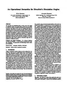
A complete model of a DH consumer is a model as sketched in Figure 2.1. The inputs are supply temperature, time and climate parameters as can be seen in Figure 2.2. The outputs are the heat load and the return temperature. The ultimate goal is developing appropriate models of the DH consumers’ dynamic behaviour.
Figure 2.1. A schematic diagram of a DH system.
3
Figure 2.2. A Complete model of a DH consumer.
The most important output is dynamic heat load. But as changes in the heat load both can occur as changes in the flow of the DH water and as changes in the cooling of the water, also the return temperature must be regarded as a dependent variable. 2.1.2
Modelling of the heat load
2.1.2.1
Models based on weighing of different input variables
Q = k1 P1 + k 2 P2 + ... + k n Pn Where:
(2.1)
Q
= Heat load P1 ...Pn = Variables affecting the heat load
K 1 ...K n = Constants The constants are either estimated from measured data by regression analysis, or through analytical work. 2.1.2.2
Pure simulation model
Model S1 As it now has been determined on which form the climate variables shall appear in the model, the final formulation is as following:
Qet = k1 + k 2Tat + k 3Tm2t + k 4 (T1 − Tat ) wt + k 5 st + k 6 ∆Ts + Fwd + Fwe Where:
Qe = Estimated heat load Ta = Ambient air temperature w = Wind velocity Ts = Supply temperature Ti = Mean indoor temp, assumed to be 20°C Tm = Weighted temperature of previous air temperatures ∆Tst = Tst – Tst-1
The systematic cyclic variations are modelled by Fourier expansions.
4
(2.2)
2.1.2.3
Prediction models
One possibility of improving the results obtained with the simulation model S1, is to use some kind of auto-regression, i.e. to use the information in the auto-correlated errors that occur when using model S1, or to deal directly with the systematic variations in the heat load. Model for 24-h prediction The following model, i.e. model A1, is similar to model S1, except that the model error 24 hours ago is taken into consideration. Thus, first an expected heat load is calculated by a model equivalent to model S1, and then the predicted heat load is corrected according to the difference between the simulated value and the value measured 24 hours ago. Model A1
Qe t = Qe*t + (Q T −96 − Qe*t −96 ) ⋅ a96 Where:
(2.3)
Q = measured heat load a96 = Constant
a96 is a constant which is estimated together with the rest of the model constant. It determines how much of the previous error is to be added or subtracted from the simulated value to obtain the best estimate of the heat load. Here 15 minutes data are being used, i.e. 96 data points for one day. Model for 1-h prediction
Following model is the same as model A1, except that here information on the error between simulated and measured values one hour ago is used to correct the heat load prediction. Model A2
Qe t = Qe*e + (Q t −4 − Qe*t −4 ) ⋅ a4 + (Q t −96 − Qe*t −96 ) ⋅ a96 Where:
(2.4)
a4, a96 = Constants
It appears that the 1-h prediction is more accurate than the 24-h prediction, although the improvement is very small for some of the substations. 2.1.3
Modelling of the return temperature
The modelling of the return temperature should be based primarily on the supply temperature and the heat load as input variables. The heat load is an independent variable in the return temperature models. The primary supply temperature measured at the substations is in many cases not the consumers' real supply temperature as the secondary supply temperature may be regulated at each individual block of flats. This regulation is frequently based on time of day and the ambient air temperature. The return temperature depends in a non-linear way on the heat load and the supply temperature. In spite of this, only a linear dependence will be assumed in order to simplify the calculations.
5
Pure simulation model
Tre t = k 1 + k 2 Ts t + k 3 Ts t −1 + k 4 Ts t − 2 + k 5 Ts t − 3 + k 6 Q t + k 6 Q t + k 7 Q t −1 + k 8 Q t − 2 + k 9 Q t − 3 + k 10 Tm 1 + Fw
(2.5)
where: Tre = Estimated return temperature Ts = Supply temperature Q = Heat load Tmlt = Tmlt-1⋅λ1+Tat⋅(1-λ1) Including one Fourier profile improves the results considerably for some substations that it is not possible to model only on the basis of the heat load, the supply temperature and possibly the ambient air temperature. The reason is probably the time dependent regulation of the supply temperature at the consumers, e.g. night set back, and possible varying cooling in the hot water system. 2.1.4
Prediction models of the return temperature
As for the heat load models, the model accuracy can be improved by means of autoregression, giving the models the properties of prediction models rather than simulation models. The prediction models have terms included which account for previous errors in the return temperature model between simulated and measured return temperature. Model AR1
Tret = Tre*t + (Trt − 4 − Tre*t− 4 ) ⋅ r1 + (Trt −96 − Tre*t−96 ) ⋅ r 96
(2.6)
where: Tr = Measured return temperature [°C] r1, r4, r96 = Constants 2.1.5
A complete model of a DH consumer
A complete simulation model can now be constructed by combining the simulation model of the heat load and the return temperature. A complete prediction model for the DH consumers is obtained by combining the predictions of the consumer's heat load and return temperature The prediction of the consumer's heat load and return temperature is essential in connection with real time optimisation. Both the simulation and the prediction models must be combined in such a way that heat load is calculated first and the return temperature is determined afterwards. Errors in prediction or simulation of the heat load thus can affect the accuracy of the return temperature calculations, but as the calculated heat load in most cases differ only a little from the actual heat load, this should not cause any serious problems. 2.2
Steady state analysis of DH networks
2.2.1
Introduction
Steady state analysis of hydraulic networks is of interest not only in network dimensioning and steady state simulation but also in dynamic simulation since having the flow distribution in the network is a precondition of pseudo-dynamic simulation by the physical models, which will be discussed in Section 2.3. In other words, steady state analysis is necessary part of dynamic analysis of DH network by the physical models.
6
In practice there are two problems, which seem to be most concerned with steady state analysis of networks. One is the convergence property and another the calculation time. DH networks differ from most other hydraulic networks in the way that they normally consist of two parts: the supply and return pipes. In most cases, the supply and return pipes are identical and flow rates and pressure losses in the supply and return pipes are nearly the same. Furthermore the pressure distribution in one half of the network does not affect the other half because the flow rates are controlled by the user’s control system. Therefore calculations for the network can normally be simplified such that only one half of the whole DH network is considered when calculating network flow rates and pressure. In this analysis, only one half of the DH network is considered. This simplification does not imply any restriction or inaccuracy in the analysis. If there are differences in connections or pipe dimensions between the supply and return pipes, each half can be calculated separately. Therefore calculations for a DH network can be made in the same way that they are made for a single pipe distribution network. 2.2.2 2.2.2.1
Existing methods Linear theory method
The basic idea of the linear theory is to transform L non-linear energy equations into linear equations and then solve the system of equations together with J-1 linear continuity equations. 2.2.2.2
Newton-Raphson method
The so-called Newton-Raphson method is widely used because it usually converges rapidly to the solution. The Newton-Raphson method may be used solving any of the three sets of equations describing flow in pipe network, i.e. the equations considering: (a) the mass flow rates in pipes unknown; (b) the corrective mass flow rates in loops unknown; (c) the pressure levels in nodes unknown. 2.2.2.3
Hardy Cross method
The oldest and perhaps the most widely used for analysing pipe networks is the Hardy Cross method. In the pre-computer days, hand solutions of pipe networks used the Hardy Cross methods, and even today many computer programs are based on this method. The method can be applied to solve the set of head equations, or the set of corrective loop flow equations, and also to solve the flow equations. 2.2.2.4
The basic circuit method
In principle the so-called basic circuit method is the Newton-Raphson method associated with considering the corrective mass flow rate in each loop as unknown. The difference is that the knowledge of graph theory is used in the basic circuit method. 2.3
Dynamic modelling of DH networks
2.3.1
Introduction
The methods used can generally be put into two classes. - Modelling the physical structure and behavior of the system. - Mathematical modelling using statistical black-box methods.
7
The dynamics of the distribution network usually affect the operation of the DH system heavily. This is both due to the time delays in the DH network, which are usually large compared with time delays in other parts of the DH system. Not only the distance but also the heat capacity of the DH pipes affects the time delays. 2.3.2 2.3.2.1
Classes of dynamic models Fully dynamic model
This category includes methods where both the temperature and the flow situation is simulated dynamically by solving the basic differential equations for heat and mass conservation, as well as the momentum simultaneously. Thus the time step used has to be relatively short, typically 0.5 – 2 seconds. The pressure and flow changes spread in the DH networks far faster than temperature changes. As the temperature variations are most important in an operational optimisation, the use of fully dynamic models to simulate the network is presumably irrelevant, due to the unnecessarily short time steps demanded if the dynamic flow variations are to be simulated. 2.3.2.2
Pseudo dynamic model
Pressure (and flow) changes spread in DH networks around 1000 times faster than temperature changes, as pressure waves travel with the speed of sound in water, approximately 1200 m/s, while temperature variations travel with a speed close to the flow velocity of the DH water. This leads to the fact that the dynamics of the flow in the network are of minor importance compared with the dynamics of the temperature changes, from an operational optimisation point of view. On this basis, the present study concentrates on methods where only the temperature is considered, socalled pseudo-dynamic methods. Thus the principle of the pseudo-dynamic method is that a new flow situation is determined by steady-state flow calculations at regular time intervals, based on the heat load and the actual supply temperatures at the individual consumers. Between each flow calculation, the flow is assumed to be constant and the transient temperatures are calculated dynamically in a number of time steps within each time interval, giving as result a new set of temperatures to be used in the next flow calculation. 2.3.3
Physical models
An important feature of the physical models is that once being verified, they can be applied to other similar systems. Furthermore they are, in general, easy to interpret and helpful to process understanding. On the other hand, the models demand the data on the physical structure of the network and the flow and cooling data of each consumer. Both sets of data may not usually be easily obtained. In general the following assumptions are used in physical models • • •
the hydraulic dispersion is disregarded heat conduction in the axial direction is disregarded dissipation is disregarded
2.3.3.1
The element method
The actual pipe is divided into a number of elements in the axial direction. Each element is typically divided into four sections where the core is the DH water, the second section consists of the steel pipe, the third section is made up of the insulation materials, and the fourth section consists of a cylinder of the soil surrounding the pipe.
8
The temperature of all sections in all elements, as well as the flow velocity of the water, the inlet water temperature and the temperature in undisturbed ground, the transient temperatures in the pipe can be simulated by calculating new temperatures for all sections in all elements successively for a chosen time step, by solving the heat balance equations. The element method proved to be quite heavy and to demand relatively long calculation time if satisfactory results were to be obtained. It is in particular problematic to use when the flow situation changes frequently, due to the need of predetermined simulation periods. The Courant number When using the element method, it is necessary to take the so-called Courant number into account. The Courant number is calculated as:
Cou =
tu x
(2.7)
where: ∆t = Time step [s] ∆x = The element length [m] u = The flow velocity [m/s] -
Cou = 1: gives the exact result. Cou ≈ 0 (i.e. small time step or low water velocity): results in excessive artificial diffusion.
Heat Capacities In order to determine temperature dynamics in each of the three parts (water-steel, insulation and ground), total capacities for the pipe section are given as
C ws = ∆x C i = ∆x
π 4
π
C g = ∆x
4
π 4
( Di2 ρ w cp w + ( Do2 − Di2 ) ρ s cp s
(2.8)
((( Dm − 2 Ds m ) 2 − Do2 ) ρ i cpi + ( Dm2 − ( Dm − 2 s m ) 2 ) ρ m cp m )
(2.9)
(( D g2 − Dm2 ) ρ s cp g
(2.10)
C = Heat capacity in one element ρ = Density cp = Specific heat capacity
[J/°C] [kg/m3] [J/(kg⋅°C)]
Heat balance equations
Cws 0 0
0 Ci 0
0 T& w m& cpw ∆x w hwi ∂T + − hwi 0 T& i + 0 ∂x 0 C g T& g 0
− hwi hwi + hig − hig
T w 0 − hig T i = 0 hig + hgu T g hguT u 0
(2.11)
where
∂T T& denotes the time derivative . ∂t
9
2.3.3.2
Node method
The node method is to use temperature values at different time-steps to determine the temperature situation. This is different from the element method, where the temperature at each time step is determined only from the time step before. The principle of the node method is, that it keeps trace of how long time a water mass, which in the actual time step arrives at a node, has been on its way from the last node. Based on time series for the temperature history of the different nodes the temperature of the mass at the inlet of the pipe is calculated, and on the basis of this as well as the heat loss and heat capacity of the pipe, the temperature of the mass at the outlet of the pipe is evaluated. In this manner a new temperature for all nodes in the network can be calculated in every time step, i.e. it is not necessary to simulate every pipe in a predetermined period as is the case for the element method. Simplifications The following general simplifications are used in the node method. • • • •
Hydraulic dispersion, axial heat transmission and dissipation are neglected. Instant mixing is assumed in nodes where two or more flows meet. The heat resistance between water and steel pipe is neglected. The heat capacity of the insulation, the mantle and the ground is neglected (special for the node method)
2.3.3.3
Comparison of element method with the node method
Computation of a temperature: • Element method: along the pipe. • Node method: in one single point. Calculation time: • Element method: proportional to the square of the number of elements. • Node method: rises 50% when the length of the pipes is doubled. 2.3.4 2.3.4.1
Statistical models Neural network model
Neural network method is used for estimation of the state of a district heating (DH) network. The advantages of a statistical model compared to a physical model are a more simplified updating and easier operation for the state estimation of the district heating network.
Figure 2.3. Structure of the neural network.
10
Calculation in neural networks is done with modules connected to each other, which are called neurones. Every neurone has a weight, which defines the connection between two elements. By connection results of all neurones we have a result of neuron layer. There might be several neurone layers, where the result of former layer is an input to next layer. Every layer consists of weight matrix, bias vector and filter, which modify the output of matrix and bias vector. The filters can have features of tangential, logarithmic and linear function. The last neuron layer gives the output of the mode as shown in Figure 2.3. The first neuron layer filter is tansig, which describes vector (a1 = tansig(W1 x p + b1)) from (-∞, +∞) to (-1, +1) as an output to the second neurone layer. The second filter is purelin and the output is a2 = purelin(W2 x a1 + b2). Dimension of the input is S1 x R and the output S2 x 1. S1 and S2 are number of neurons in first and second layers. A one dimension ( R) of first layer is a function of input. The second dimension (S1) is decided by user. After designing the output dimension (S2) of the model all dimensions of neuromatrix and bias vector are fixed. Time series model contains usually two parameters to one output and some parameter to input, but neural network model has parameters of S1 x (R+1) + S2 x(S1+1). The parameters have their values in learning mode, where the learning algorithm calculate interactively the values of coefficients, which minimise the variance between output and measuring data. 2.3.4.2 •
X(eXtraneous) model
ARMAX (Auto-Regressive-Moving-Average-eXtraneous) model
A(q -1 )y(t) = B(q -1 )q -k u(t) + C(q -1 )e(t) Where: •
(2.12)
e(t): Gaussian white noise k : Time delay between input and output
If A(q-1)=1 and C(q-1)=1 → X model: y(t) = B(q-1)q-ku(t) + e(t) - simple and easy to use
Gives good results except when: - Supply temperature is abruptly changed - Different night set back strategies are implemented - DH water velocity is extremely small 2.4
Simplified dynamic models of DH networks
2.4.1
Existing simplified DH network models
2.4.1.1
Stochastic critical point model
The model is based on the assumption that it is possible to find several representative points (critical points) in a network and when the supply temperature demands at these points are satisfied, the supply temperature demand in the whole network is ensured. 2.4.1.2
Equivalent network model
An equivalent model of DH networks using a few consumers and a few pairs of pipes to represent a complete network is and attractive idea. The simplified model, referred to as an equivalent network, is generated by gradually reducing the topological complexity of the original network. 11
During this reduction, the relevant model parameter of the network are transformed in such a way that the dynamic behaviour of the equivalent network will resemble the original one. 2.4.1.3
A combined critical point and equivalent network model
A simplified dynamic DH network model which can be incorporated in e.g. study of DH system operation should describe not only the most unfavorable points in the network in order to guarantee the satisfaction of the consumers’ heat demands, but also the heat loss from the network, the pumping power consumption and the heat storage capacity of the network in order to consider the network in the optimisation of DH system operation. This can be done by the following procedure: 1. Determine the critical points in the network. 2. According to the locations of the critical points, divide the network into sub-networks. 3. Keep the sub-network where the critical points are located unchanged. 4. Aggregate the sub-networks where no critical point is located into e.g. one consumer - one pipe network. 2.4.2
An aggregated model based on the structure of the network
2.4.2.1
Principle
The following assumptions are used: • • •
All technical data of the pipes are known and the network is a tree type network. The supply and the return pipe are identical and isothermic. All consumers have the same cooling of the DH water.
2.4.2.2
Parallel connection
Figure 2.4. Two typical connection cases.
In this case mass flow in the equivalent pipe should be calculated as follow:
m = m1 + m2
(2.13)
V = V1 + V 2
(2.14)
The heat loss of the equivalent network should be equal to the heat loss of the real network namely Q = H ⋅ t s = H1 ⋅ t s + H 2 ⋅ t s 12
(2.15)
therefore
H = H1 + H 2 2.4.2.3
(2.16)
Serial connection
In the serial connection case, the following equations apply: Mass flow: m = m1 = m2 Flow rate: V = V1 + V2 Heat loss: H = H 1 + H 2 Length of the equivalent pipe: Le =
Vw
π
4
(2.17)
De2
Heat loss coefficient of the equivalent pipe:
h = H/L e 2.4.3
(2.18)
Collecting nearby nodes
Loads may be present at both ends of branch 2 as indicated in the figure. We will divide branch 2 in two parts and let branch A represent branch 1 and the first part of branch 2 while branch B shall represent the other part of branch 2 and branch 3. In this section we will use µ to indicate flow in branches while m as in the previous sections indicates flow to heat exchangers. This leads to the following identities.
Figure 2.5. Collapsing Nodes.
m1 = µ 1 - µ 2
(2.19)
m2 = µ 2 - µ 3
(2.20)
Branch 2 is divided into two parts with the length fAL2 and fBL2 f A = m 2 /(m1 + m 2 )
(2.21)
13
f B = m1 /(m1 + m 2 ) = 1 - f Α
(2.22)
Branch A and B are defined by LA = L1+fAL2
LB = L3+fBL2
V1 p + f AV2p ϕ A = 1 + X V + f V A 2 1
−1
V3p + f BV2p ϕ B = 1 + X V3 + f BV2
−1
µA ϕA µ ϕ + f AV2 A A µ1 ϕ 1 µ2 ϕ2
VB = V3
µB ϕB µ ϕ + f BV 2 B B µ3 ϕ3 µ2 ϕ 2
1−ϕ A ϕAX
VBp = VB
1−ϕB ϕAX
dA = 2
VA πL A
dB = 2
VB πLB
DA = 2
VA + VAp πL A
DB = 2
VB + VBp πLB
V A = V1
V Ap = V A
hA =
h1L1 + f A h2 L2 LA
2.4.3.1
hB =
(2.23)
h3 L3 + f B h2 L2 LB
Case study: Hvalsoe district heating system
Hvalsoe is a small town located in the centre of Zealand in Denmark, cf. the description in Chapter 4. 2.4.3.1.1
Models of the DH system
To verify the accuracy of the method for creating equivalent systems, several models of the Hvalsoe DH system are made and compared by simulations. The following systems have been modelled and simulated: A The original system with 535 loads and 1079 branches. A pure tree structure. B An equivalent system with all 535 loads and 1079 branches-but no side branches. C1 to C12 Reduced equivalent systems, which is created by removing the short branches of model B. Systems with 500, 200, 100, 50, 25, 12, 6, 5, 4, 3, 2, and 1 branch, are modelled. D1 to D3 An equivalent system generated by dividing the original system in model A into 24 sub-systems (see Figure 2.6) each of which is then transformed to a structure with no side branches and subsequently reduced to 10, 5, and 1 branch (This results in 201, 108, and 24 branches, respectively).
14
Figure 2.6. Grouping of the Hvalsoe district heating system.
2.4.3.1.2
Simulations
The simulations cover a period of 24 hours with step of 2 minutes. Time series for the 535 heat loads are calculated by scaling a measured time series of the total load at the plant with the yearly loads at each consumer. The results are summarised in Figure 2.7.
Figure 2.7. Standard deviation of error in return temperature for models B, C1 to C12, and D1 to D3 as compared to models A (the original system).
Figure 2.7 shows that the number of branches in the equivalent network can be reduced to approximately 10 branches without affecting the accuracy. If more branches are removed the error increases more significantly. For a description of the German network aggregation method, refer to Chapter 3. 2.5
Optimisation of DH system operation
2.5.1
Introduction
The goal of optimum operation of a DH system is finding the most economical way to fulfil the consumers’ heat requirements, given the physical construction of the system, the consumers’
15
dynamic heat load and the time-dependent electricity price ce. In the Optimisation of DH System Operation, the minimising of the cost of the DH company is considered. One of the important aspects to model is the start and stop of different heat production units. Another important aspect is the distribution of the heat production between the different production units (load dispatch), assuming that there are more than one unit in the system. The third aspect could be the regulation of the supply temperature from the plant(s).
Figure 2.8. The principle structure of the operation of a DH system.
As indicated in Figure 2.8, an optimisation of DH system operation is defined as the process of determining which combination of heat production of different units (unit commitment and load dispatch) and supply temperature from different plants (supply temperature control) leads to the lowest costs, when the heat load forecast, the cooling of the DH water and the time dependent electricity price ce are given throughout the chosen horizon. 2.5.2 2.5.2.1
Existing models and methods Models considering unit commitment and load dispatch
In this case the problem has been simplified by disregarding the sub-problem of the supply temperature control. The task of the problem is then to determine the start and stop of different heat production units and the load distribution among them. In this case, the general features of the program are as follows: • • • •
The supply temperature Ts is predetermined. The hydraulic regime of the DH network is controlled by the critical point method. The dynamics of the network is disregarded. The task is to determine the start and stop of different heat production units and the load distribution among them (unit commitment and load dispatch).
2.5.2.2
Models considering load dispatch and supply temperature control
In order to improve DH system operation by considering the dynamics of the network, the supply temperature control becomes necessary. The problem of the load dispatch and the supply temperature control has the following features: • • •
16
The hydraulic regime of the distribution network is controlled by the critical point methods. The task is the load dispatch and the supply temperature control (at DH plants). The dynamics of the network is considered.
2.5.2.3
A minimum supply temperature control strategy
In this strategy the unit commitment and load dispatch are disregarded. In other words, only the supply temperature control is considered. The following assumptions are made in the method: • • • •
The hydraulic regime of the network is controlled by the hydraulic critical point method. The base load unit is sufficiently big, therefore the unit commitment and the load dispatch can be disregarded. The pumping cost is disregarded. The supply temperature at DH plants should be kept as low as possible. In other words, lower supply temperature is interpreted as lower operation costs.
2.5.3
Optimisation Models
A standard optimisation problem: Min f(x) g(x) ≤ b h(x) = c
where f(x) g(x),h(x)
cost function constraints
Cost function to be minimised: M
Qh Pb τ Qbt cc + t c g + t ce,t ) ηh ηp ηb
∑ 60 (
Min
t =1
(2.24)
t = 1,…, M where: M
decision horizon
cc
coal price, DKK/kWh
cg
gas price, DKK/kWh
ce,t
electricity price
Q
heat production, kW
P
power consumption, kW
η
efficiency
∆τ
time interval, minutes
b
base load production
h
peak load production
p
pump
Subscripts:
An optimisation model of DH system operation will be presented to show how the sub-models of each component are integrated into an optimisation model.
17
The formulation of the optimisation problem of DH system operation with a boiler plant with limited base load capacity may be modified or simplified in the following aspects: 1. X model: represent the relationships between the supply temperature at the DH plant and the supply temperatures at the consumers.
Ts p,i,t − a1i − a 2 i ⋅ Tst − ni +1 − a3i ⋅ Tst − ni − a 4 i ⋅ Tst − ni −1 = 0 ; i = 1,2,....,I
(2.25)
where: I
number of substations
a1i,t, a2 i,t, a3 i,t
time-varying parameters
2. Assuming the prediction of the return temperature at each substation is available and it does not depend on the supply temperature at the relevant substation.
mi ,t −
Qi ,t cpw (Ts p ,i ,t − Trp ,i ,t )
=0
(2.26)
where m
mass flow of the substations, kg/s
Q
heat load of the substations, kW
cpw
specific heat capacity, kJ/(kg°C)
k1, k2, q
constants
3. Assuming the prediction of the return temperature at the DH plant is available. I
Qpt − ∑ mi ,t ⋅ (Ts t − Trt ) + Pp t = 0 i =1
where
(2.27)
Qp total heat production of the system, kW
4. Considering the effect of the past operation decisions before the decision horizon starts as follows:
Ts j − ni = Tsi j − ni j = 0,1..., ni ni = max[ni ]
(2.28)
Where: T si j−n i is the measured supply temperatures 5. Considering the effect of the past operation decisions before the decision horizon starts as follows
18
Ts j ≥ Ts j , min
j = M − n i ,...M
(2.29)
Ts j ≤ Ts j ,max
j = M − n i ,...M
(2.30)
6. The resistance coefficient of the system
snet = 2 ⋅ ∑ s j ⋅ r j
(2.31)
j∈P
2.5.4
Possible solution methods
Since some constraints, e.g. the constraints induced by the network, depend on the supply temperatures that are among the decision variables of the optimisation problem, an iterative solution procedure could be a possible solution method. The iterative solution procedure The basic idea of the method is to use a dynamic network simulation model to determine the relationships between the supply temperature at the plant and the supply temperatures at the individual consumers, on the basis of a starting guess on the level of the supply temperature. In the same way the resistance coefficient of the network is used, and the return temperature at the plant can be evaluated. The problem then is to be solved with methods suitable for constrained minimisation. After each minimisation, a new value of the supply temperature in every time step of the optimisation period would be one of the outcomes, and this supply temperature then can be used as an input in a new dynamic simulation, resulting in a new set of equations and a new optimisation problem. If successful, this method would result in converged supply temperature (i.e. the resulting supply temperature is in every time step unchanged between two successive iterations), and thereby the determination of an optimum operational strategy for the chosen period. The principles of the outlined method appear from the flow diagram as follows.
Figure 2.9. The iterative solution procedure.
19
The advantage of iterative optimisation method The iterative optimisation method is more flexible and it is easier to include new constraints than is the case in the searching method, as well as increasing the number of decision variables or extending the optimisation horizon will presumably not have as dramatic effects on the calculation time as is the case for the searching method. 2.6
Software
2.6.1
The software system BoFiT
2.6.1.1
Introduction
2.6.1.1.1
The optimisation algorithm
It is based on a decomposition co-ordination principle, called resource allocation which involves mixed integer linear programming. 2.6.1.1.2
Structural conception
From the beginning BoFiT has been considered as a toolbox, providing a flexible, easily adaptable and expansible framework for software modules applicable for special tasks which enables the experienced engineer to work out the optimal operation strategy for a given DH system stepwise. BoFiT/SIM
Dynamic network simulation module
BoFiT/TEP
Optimisation tool for unit commitment And economic dispatch
BoFiT/POP
Minimisation of pumping power consumption
BoFiT/VTO
Dynamic optimisation of supply temperature
BoFiT/ERGO
Mid-Term operation planning
2.6.1.1.3
The features of the BoFiT modules
The development of BoFiT has begun with the implementation of a dynamic network simulation module(BoFiT / SIM) and an optimisation tool for unit commitment and economic dispatch (BoFiT / TEP). The following development of the modules BoFiT/POP for minimisation of pumping power consumption, BoFiT / VTO for dynamic optimisation of supply temperatures and BoFiT / ERGO for mid-term operation planning can be regarded as continuously filling the space between simulation of the distribution subsystem to mid-term resource scheduling for the whole supply system. While BoFiT / VTO and BoFiT / ERGO are still in state of development, the other modules are available for UNIX platforms. All modules interact with a central relational database system and are accessible from a common graphical user interface, that provides database management, security, protocol and help functions.
20
SIM
VTO
TEP
NLP
MILP
Online
Daily
Daily
operation
planning
planning
Yes
yes
Yes
No
No
Dynamic
Mathematical method
simulation
Preferred usage conditions
Studies
DH network dynamics
POP Dynamic simulation & MILP
ERGO
Decomposition & MILP
Annual planning
Model
Cogeneration
No
no
Yes
Yes
Yes
covers
Plant dynamics
No
no
No
Yes
Yes
No
no
No
No
Yes
Result
result
Result
-
-
Input
result
Result
-
-
mid-term contract conditions Pressures, temperatures & flows in the DH network Set points of pressure controllers Supply temperatures
Occurring
Input
input
Result
Input
Input
Input
input
Result
Result
Result
Unit commitment
Input
input
Input
Result
Result
Load forecast
Input
-
Input
Input
Input
Online process data
-
input
(input)
(input)
-
Dispatch
2.6.1.2
as
Minimisation of pumping power costs
When measured data from SCADA (pressures, temperatures, flows) are introduced on-line into the model equations, the DH network simulation turns into an instrument of state-estimation. This instrument is useful to reveal critical locations concerning pressure differences visualise the extents of supply areas belonging to a certain plant and monitor the real consumers’ load. For the automatic adaptation of the controller set points for pumps and valves automatically respect to minimal pumping power consumption the DH network simulation was enhanced by an optimisation model in Indenbirken, M., Tröster, L. and Steiff, A. (1995). First an analysis procedure divides the network into areas, that are dominated by a certain controller e.g. a pressure difference controlling pump. For each area critical points, characterised by e.g. minimal pressure, minimal pressure difference, pressure reaching the maximum permissible value or conditions near the boiling point of water, are identified. 2.6.1.3
Unit commitment and economic dispatch
The BoFiT / TEP model aims at minimisation of operating costs caused by purchase of fuels, heat and power delivered by third parties. The complete path of energy conversion is modelled, starting at consumer's demands (heat, power, steam), heading via transport (e.g. hydraulic restrictions, pumping power consumption), storage (e.g. tanks, storage power stations), conversion (e.g. steam boilers, gas turbines, steam turbines, condensers) and contracts (fuels, heat, power) to the objective function (sum of costs). The system structure is represented by a graph consisting of technical and economical elements and streams (water, steam electricity, costs), that is provided to BoFiT / TEP using a graphical configuration tool. The model is solved by linear programming, and the branch-and-bound procedure provided by a commercial solver.
21
2.6.1.4
Mid-term operation planning
Mid-term operation planning of energy supply systems, usually ranging up to one year, exceeds the scope of daily unit commitment and economic dispatch according to BoFiT/TEP as technical and economical mid-term constraints have to be considered, which mostly result from terms of energy purchase or delivery contracts, e.g. limited quantities of heat, power or fuel. Several algorithmic approaches like Dynamic Programming, Lagrangian Relaxation and MILP have been suggested for mid-term optimisation. MILP is particularly suited for model building of energy systems including combined heat and power (CHP) generation plants and DH networks, as approximate modelling of technical essentials e.g multi-level steam extraction from turbines, sequential preheating and hydraulic transport restrictions is possible.
Figure 2.10. Solution strategy for mid-term operation planning.
2.6.2
APROS (Advanced PROcess Simulator)
For a description of the APROS simulation environment, refer to Section 5.2.
22
3 Oberhausen District Heating System
3.1
Introduction and target of the work of Fraunhofer UMSICHT
Within complex optimisation strategies for energy supply systems, like dynamic supply temperature optimisation, the transient characteristics of the heat transport in the DH network are modelled using the mathematical form of non-linear optimisation. The DH network appears as set of constraints in an optimisation model where the technical restrictions and the systems operation have to be included. The objective function contains the fuel costs for heat and power, and the costs of heat and power purchases. The approach developed at Fraunhofer UMSICHT connects separate production plant, network and contract models to an overall model of the complete energy supply system. Not only the district heating sector but also the electricity part of the system is regarded. Consequently the optimisation results may contain complex effects, e.g. the usage of heat storage in the network in order to operate cogeneration plants in a way that the purchase of electrical energy is reduced in times of high tariffs. Special consideration has been drawn towards an accurate modelling of the district heating system. Every element (pipe, consumer, valve etc.) is modelled separate and mathematically connected by graph methods (cf. Park et al. (2000), pp. 138-139). It is obvious that an optimisation model of a large system with many loops and more than one heat plant will easily reach a difficulty, which exceeds the scope of current algorithmic and computational resources. So network aggregation has to be applied in order to reduce the problem size. The simplified network models have to correspond to the detailed models concerning pressure distribution and heat transport dynamics with sufficient accuracy. Within the work of Fraunhofer UMSICHT in this project the effects of aggregated network structures on simulation and optimisation results have been analysed. For this purpose exemplary the DH system of the local energy supplier Energieversorgung Oberhausen AG (EVO) has been regarded. To determine whether DH network aggregation will lead to advantages for future energy supply companies Fraunhofer UMSICHT based their work on the simplification strategy developed by Loewen (2001) and the non-linear optimisation approach of Tröster (1999). The level of network aggregation had to be chosen so that a significant advantage in computational efficiency is obtained while an acceptable model accuracy is maintained concerning the significant technical properties like pressure-, flow distribution, and time delays in the DH network. 3.2
Principles of aggregation
Within this chapter only a short review on the principles of the aggregation method for DH networks to be regarded in this project should be given. A detailed description is given in the State of the art report. The consideration of all components of the district heating network is in many cases not needed. Often only the overall network characteristics or the behaviour of a few components are interesting for the load management or for the application of optimisation methods. Therefore, at Fraunhofer UMSICHT an approach has been developed which enables the automatically simplification of complex DH networks. The following requirements are necessary for an efficient simplification strategy: •
With the same input parameter (Supply temperature, heat and electricity input etc) the operational characteristic of the entire system, including the network, should not change.
•
It must be possible to exclude special nodes and components (e.g. control nodes or critical points) from the simplification.
•
Aggregation should be possible to each level of simplification.
•
The mathematical relations of the separate network models (pipes, valves, and consumers) should not be affected by the aggregation. This guarantees the compatibility of the aggregation method to other simulation and optimisation tools.
23
•
Control strategies for the not aggregated DH network should be also applicable for the simplified network.
•
The visual appearance of the DH network should be kept as long as possible. That means the remaining nodes should not change their geographical coordinates.
The developed method enables the restructuring of nodes, consumers and pipelines within the model of the DH network. This is done in accordance with the thermo-hydraulic laws and the heat and mass balances. Afterwards, the configuration parameters of the remaining components are adjusted so that the network’s mass flows, pressures, temperatures and delay times are as good as possible in accordance with the original network model. This ensures that the overall energy balances with regard to energy input, heat storage, heat losses and pumping power fit to those before the simplification. Active elements (production units, pumps, valves, and heat exchangers) should not be eliminated since supply temperature optimisation is intended to improve the operation of these elements to reach a global optimum of the entire DH/CHP-system. In the strategy developed at Fraunhofer UMSICHT the computer model of a district heating network exists of submodels for each separate element (production unit, pipes, consumers, etc.). The functions describing these submodels are not affected by the aggregation. This ensures that the simplification strategy is applicable to different network models and simulation/optimisation platforms. To carry out an aggregation the complete network has to be modelled with a simulation tool. At Fraunhofer UMSICHT the simulation and optimisation tool BoFiT is used, Icking et al. (1992). Additionally, operational data determined by simulations is needed to adjust the parameters of the aggregated system so that the characteristics of the simplified network are in accordance with the original network. The exactness of the aggregation can be determined by a comparison of simulation results of the not simplified system with those of the original system under the same control conditions. 3.2.1
Mathematical fundamentals
For a separate pipeline the interaction between pressure difference ∆p and mass flow described by the Darcy-Weisbach law •
•
m is
•
∆p = m⋅ m ⋅ r − ρ ⋅ g ⋅ ∆h
(3.1)
The constant r is given by
r=
l ⋅ ⋅ξ R + π ⋅ ρ ⋅d d 8
2
4
∑ξ
zus
(3.2)
With the parameter ξzus additional resistances like elbows etc. are considered. The friction ξR has to be calculated in dependency of the flow characteristics. E A The mass flow of a consumer is calculated by the input and output temperature TVB and TVB , the specific heat capacity of the district heating water cp,W as well as the time dependent heat load •
Q VB . •
mVB =
24
•
QVB
(
E A c p ,W ⋅ TVB − TVB
)
(3.3)
For the outlet temperature TA of a fluid after flowing through a pipe of the length l, the diameter d and the heat transfer coefficient k the following equation is valid. The outlet temperature is calculated in dependency of the pipes input temperature TE and the temperature of the environment T U:
T
A
=T
U
(
+ T −T E
U
π ⋅ k ⋅l ⋅ d ⋅ exp − • c p ,W ⋅ m
)
(3.4)
Nodes within the network structure usually have got more than one input mass flow what leads to a mixing of these mass flows. It is assumed that an immediate and total mixture leads to constant outlet temperatures of the node. The temperature of this mixture TK can be calculated with
TK =
n
i =1
• E E i ⋅ Ti
∑ m n
∑
(3.5)
• E mi
i =1
The number of incoming mass flows is n. It is assumed that all mass flows have the same heat capacity. The time delay τ between input and output of an infinitesimal water element is calculated in •
dependency to the volume V, the mass flow m and the density ρ of the district heating water
τ=
V ⋅ρ
(3.6)
•
m 3.2.2
Aggregation of the different sub structures
The model of a district heating network consists of diverse sub structures. The development and application of different algorithms for the network simplification depends on how the components to be eliminated or combined are connected. Basically, it is distinguished between four different sub structures: 1. Blind elements and nodes (in operation not connected to the network) 2. Serial pipes 3. Branch pipes (here often called “forks”) 4. Loops All nodes and pipes, which are useless for the thermo-hydraulic simulation or optimisation of the system, will be eliminated in a preliminary simplification step. These are nodes, which are not connected to any element, elements, which are only connected at one side to another element and nodes, which connect pipes with the same diameter where no consumer is connected.
25
serial pipes
Simplif icat ion
branch pipes
loops
Figure 3.1. Different sub structures in a district heating network.
The other algorithms for the sub structures described above are applied iteratively until the desired aggregation depth ϕ has been reached.
ϕ = 1−
Number of elements in aggregated network Number of elements in original network
3.2.3
(3.7)
Combination of serial pipes
Nodes between two pipes which both have the same flow direction and where only one consumer is connected to can be eliminated. The nominal load of the consumer is distributed among the two neighbouring consumers and the two pipes can be combined to one (Figure 3.2). This strategy eliminates three elements and two nodes each time it is applied to the DH network. With the right parameter adjustment and distribution of the consumer’s heat load no error occurs for steady state calculations and for dynamic purposes the errors are very small. a) Sub structure before aggregation
b) Sub structure after aggregation
Supply line K3V
R1V
K1V
VB2 R1R
VB3
VB1’
VB3’ R1R’
R2R K2R
K3V R1V’
R2V
VB1
K1R
Supply line
K2V
K1V
K3R
Return line
K1R
K3R Return line
Figure 3.2. Serial pipes sub structure before (a) and after (b) aggregation.
The following requirements have to be kept as good as possible so that the thermo-hydraulic balance at the sub structures boundaries are kept. 1. 2. 3. 4. 5. 6.
26
The total volume of the pipes in supply or return line must remain constant. Constant delay times between not eliminated nodes. Constant temperatures and nodes at the not eliminated nodes. The sum of the mass flows through all consumers must remain constant. Constant overall heat load. Constant heat losses.
Taking into account the first requirement the diameter of the pipes R1’ can be calculated. The length is usually determined in a heuristic manner. With equation 3.6 from Section 3.2.1. and considering requirement 2 the mass flows in the remaining pipelines can be calculated. With the mass balances at the nodes K1 and K3 the mass flows through the consumers can be determined. On the basis of an energy balance at node K3R (Eq. 3.5) the outlet temperature at VB3’ is calculated. Now the inlet temperature, the outlet temperature and the mass flow at VB3’ are known and the heat load can be determined (Eq. 3.3). With requirement 6 consequently the new heat load of consumer VB1’ follows. Now the outlet temperature of the pipeline R1R’ has to be adjusted so that the temperature of node K1R remains constant (TK1,R‘ = TK1,R). With equation 3.4 the right heat transfer coefficient can be calculated. Pipeline R1V is calculated analogues. Finally, to ensure that the pressure at the nodes remains constant, the additional resistances (ξzus ) of the pipelines R1V’ and R1R’ will be adjusted. The right values can be calculated by inserting equation 3.1 into 3.2. 3.2.4
Simplification of branch pipes (“forks”)
Branches exist, if from a supply node mass flows flow into at least two different pipelines. The two branch pipes are converted into two serial pipes (Figure 3.3). Therefore, usually no real aggregation takes place, since the number of the elements remains constant. However, after this step the new serial pipe structure can be simplified with the serial pipe algorithm (Section 3.2.3). Sometimes the delay time of R1 and R2 are almost the same. In these cases an additional elimination step can follow the branch simplification in which the pipe R2 can be eliminated and the two consumers can be combined to one consumer with the summarised heat load. In order to ensure that after the aggregation the DH network shows almost the same behaviour as before, the same conditions as described in the last chapter must be kept. Additional the following prerequisite has to be fulfilled: 7. Only one consumer is connected to the end of branch R1.
a) Sub structure before aggregation
b) Sub structure after aggregation
K2V R1V VB2
K1V
Supply line
Supply line K3V
K3V
R1V’
R2V K2R
VB1
K2V’
K1V
VB3
R2V’
VB1
VB2
VB3
R1R R1R’
R2R K1R
K3R
K1R
R2R’ K2R’
K3R
Return line Return line
Figure 3.3. Branch sub structure („Fork“) before (a) and after (b) aggregation.
If several consumers and pipes are attached to the branch, it has to be simplified in accordance with the strategy already described. From the conditions described above it follows that the delay time in R1' has to be equal to those of R1 and the delay time in R2 ' equals those in R2 subtracted by the time in R1. The mass flows and heat loads of the consumers VB2 and VB3 remain constant. Therefore, the mass flow in R1’ is calculated by summarising the mass flows of R1 and R2. The mass flow in R2’ is the same as in R2. The calculation of the geometric parameters of the pipes, the heat transfer coefficients and the additional resistances (ξus ) has to be done analogues to the strategy described in Section 3.2.3.
27
3.2.5
Simplification of loop sub structures
Loops can be split at supply nodes where the mass flows flow together, that means where are more than one input mass flow. As presented in the Figure 3.4 the algorithms implemented yet only accept one pipe with a consumer connected downstream the loop (in the supply line). This structure is to be produced by application of the former described algorithms (combination of serial pipes and simplification of “forks”) before splitting the loop. A splitting of further downstream located pipes would be too complex and instead of a simplifying the structure it would lead to a much more complex system. However, each time a loop is split the number of elements and nodes in the network increases by four if pipe R3 exists and it increases by two nodes and one consumer if not. After splitting a “fork” and two serial pipe sub structures exist which can easily simplified with the already described algorithms. After the splitting of the loop the nodes K1V/R and also all elements in the supply line in flow direction behind this node are two times in the network. In accordance with the defined conditions (Section 3.2.3, requirements 1 - 6), the total volume of the pipes, the total consumer loads and the total mass flows should not change. a) Before aggregation
b) After aggregation Supply line
R2V
K1V
K2V
VB1
VB2
K1R
R3a’V VB1b’ VB2a’ b R3b’R
VB1a’ R2 R
K2R
R1R
Return line
K2b’V
R3b’V K2a’V
R1 V
R3R R1R
K1b’V
K1a’V
R3V
R1V R2R
R2 V
Supply line
K1b’R K1a’R
VB2b’ b K2b’R
R3a’R
K2a’R
Return line
Figure 3.4. Loop sub structure before (a) and after (b) aggregation.
Taking the requirements into account and using the equations given in Section 3.2.1 all geometric and thermo-hydraulic parameters of the pipes and consumers can be calculated analogues to the serial pipe and fork sub structures. A detailed description is given in the State of the Art Report. 3.3
Principles and aims of supply temperature optimisation
Especially for distributed systems like combined energy supply systems with renewable energies and CHP the optimal use of heat storage capabilities increases the overall efficiency. In particular for DH systems with fixed heat coupling (back pressure turbines), appropriate approaches will enable a reduction of active heating plants by the usage of the system's heat storage. Additionally, it enables the displacement of expensive peak power plants, to reduce electrical power peaks and to enable a better utilisation of tariffs. Since the DH network of an energy supply system often has a volume of more than 50.000 m3, the pipeline system in particular has a huge potential for the storage of energy at no additional investment costs. In a DH network a time of some minutes to several hours passes between the input of heat at the production plant and the output of this heat at particular consumer stations. In other words, during this time the heat is stored in the DH network. The maximal storage time depends upon the distance between the production plant and the consumer and the velocity of the DH-water. Therefore, the characteristics of the energy supply system’s operation have to be considered to evaluate the potential for heat storage processes.
28
generation and distribution costs fuel consumption generation and purchase of energy DH, CHP
CHP purchase
optimised costs
optimised load dispatch optimised unit commitment
control profiles °C
electricity area
120
load covering
100
pumping power
T v=f(t)
80 h
heat losses heat storage thermohydraulic time characteristic DH network
critical pressures nonlinear optimisation model
peak shaving less power purchase better utilization of tariffs optimisation of heat storage minimisation of fuel consumption minimisation of GHG emissions
Figure 3.5. Heat storage optimisation model.
To determine the optimisation potential of heat storage processes in DH system of a DH or CHP system, an algorithm for the dynamic optimisation is necessary. As input data, the technical and economical structure of the energy production facilities, the energy purchase as well as the DH network including heat accumulators and the prognoses of the thermal and electrical power requirements of the consumers is needed (see figure above). This prognosis data must be provided over the time period considered for the optimisation. On the basis of this data an appropriate optimisation model has to be created which enables the consideration of the dynamic thermo-hydraulic behaviour of DH and CHP systems. These characteristics are due to dynamic energy production, distribution and demand. The dynamic pumping power requirement along with the heat loss has to be modelled. Special consideration must be taken towards a suitable mathematical formulation for the complex dynamic processes in the transport system since this is essential when modelling the heat storage processes in the DH system. The unit commitment, the load dispatch as well as the operation of the bypasses and especially the supply temperatures in all heat production plants must be considered to facilitate the full potential of the energy supply system due to its optimisation by the heat storage processes. 3.3.1
Mathematical model
For the mathematical modelling the energy supply systems is divided into the areas energy supply and DH network. Under the term energy supply the enterprise owned systems for the energy conversion, the contracts for the external supply of heat and electrical power as well as the electricity networks are combined. They have to be set up in such a way that the supply temperature is received as optimisation variable. The DH network is the most important part of the mathematical model. In this model the thermo-hydraulically dynamic behaviour of the DH network has to be considered. This submodel is based on methods of the thermo-hydraulic network simulation. The basis of the mathematical model is the separation of the optimisation period into equidistant time steps with the time increment ∆t. The time steps are chronologically numbered. The starting point of the optimisation period is the first time step. To get a clearer formulation of the model the first time step is defined as zero point of the time axis. Based on this discrete representation the model is divided into three sections for the description of the thermo-hydraulic dynamic behaviour of the DH network:
29
• • •
steady state hydraulic model steady state thermal model dynamic thermal model.
Due to the assumption of a quasi steady state hydraulic behaviour of the system the steady state hydraulic model has to be set up for each time step. The steady state thermal model serves for the definition of a clear starting point for the dynamic optimisation. Due to the convective heat transport and the large delay times in some pipes a dynamic thermal model has to be developed for these components, which describes the delay time characteristic of the network. For the other components of the DH network the delay time behaviour can be neglected. 3.3.2
Objective function
With economic questions it is obvious to use the height of the attainable profit to evaluate the quality of a decision. However the incomes of the energy supply company cannot be influenced by the operation mode and therefore they represent a constant in the context of operational planning. That is why instead of the profit the operating costs can be used for the evaluation of the quality of an operation mode for the operational planning regarded in this work. As proportions of the operating costs only the costs of the energy purchase as well as of the fuel supply for the production systems are influenced by the operation mode of the power supply system. Therefore, the total costs K for the energy purchase are selected as objective function of the optimisation problem.
∑K
e ∈ GHWK
e
+
∑
Ke e ∈ GTHWK
+
∑K
e
+
e ∈ SB
∑K
e ∈ HW
e
+
∑K
e
=0
(3.8)
e ∈ WB
With GHWK: GTHWK: HW: SB: WB:
Set of production units with backpressure turbines Set of production units with gasturbines Set of production units with heat only boilers (HOB) Set of electricity purchase contracts Set of heat purchase contracts
Target of the operational planning is the determination of the operation mode with the minimum operating costs. All other equations represent secondary conditions of the optimisation problem, which have to be kept. 3.4
The EVO DH network
The applicability of the aggregation procedure was tested at a model of the DH system of the power supply company of “Oberhausen“ (EVO). This model is based on real data and by numerous comparisons between simulation results and original measuring data it was validated. The network consists of three hydraulically separated systems (“Sterkrade“, “Oberhausen” and “Schiene”). The system “Schiene” is a heat transport line, which connects the two other systems. To the DH system “Schiene” only one big consumer and a waste incineration plant with 35 MW heat and 25 MW power production is connected. Within the EVO district heating system three CHP plants are operated with a total heat and power production of 160 MW and 60 MW respectively. Besides the heat input of one CHP plant 30 MW waste heat is coupled to the northern “Sterkrade“ system.
30
Sterkrade
Schiene
Oberhausen
Figure 3.6. The district heating system of the energy supply company of “Oberhausen“ (EVO).
In the figure above the structure of the supply line of the EVO DH network is described. The return line is completely parallel to this structure. Consumers are symbolised by small points and pipes by lines. Additionally, the three CHP plants are shown. The network model consists of 2380 pipes, 1000 consumers and 2205 nodes. In the system 176 loops exist. The total pipe length is 190 km. The nine pumping stations, the armatures and the production units should not be eliminated since the operation of these elements should be optimised later on. To carry out the aggregation the network is divided into the three different systems. Each system is simplified separately. In the following the aggregation of the southern “Oberhausen“ system will be described. The complexity of this network is sufficient, in order to apply the different aggregation algorithms several times until supply temperature optimisation is applicable and to evaluate weather the aggregation error of a simplified DH network model at high aggregation degrees is low enough. 3.5
Simplification of EVO DH network
3.5.1
Description of the work process
The next figure describes the course of the modelling, aggregation and optimisation of a district heating system as done in this project. In a first step the detailed network of the EVO system had to be developed. This has been done by collection, processing and input of configuration data. The data has been used to model the DH system within the simulation platform BoFiT. To adjust the model to real behaviour a detailed set of measurement data has been collected. Besides pressures and temperatures also the delay times have been adapted as good as possible. The accuracy has been checked by steady state simulations.
31
Conf igurat ion dat a
M easurement dat a Comparison
Simulat ion plat f orm
St at ic simulat ion result s
Det ailed net w ork model
aut omat ic calculat ion Addit ional simplif icat ion
Simplif ied net w ork model
Opt imisat ion plat f orm Opt imisat ion model (GAM S) Nonlinear solver (e.g. CONOPT) no
solvable ?
Result s (Excel t ables & diagrams) Figure 3.7. Project working process.
To carry out the aggregation a detailed network model and the results of a steady state simulation are needed. Since high mass flows contribute to the reduction of rounding errors, an operation mode with a supply temperature of 118 °C and a load factor (actual load divided by nominal load of a consumer) of 60 % is applied. The return temperatures of the consumers are uniformly 50 °C. As already described, the simplification is done by applying the aggregation algorithms iteratively to the DH network. The following figure describes exemplary how the number of elements decreases during a simplification process. In this case always the iterative course started with the serial pipe elimination (Step 1). Afterwards the branch simplification (Step 2) took place and finally the loop simplification (Step 3) before it starts again with serial pipes (Step 4), etc. Each time the respective algorithm is applied to the DH network until no appropriate substructure was left in the network. 1400
Number of Elements
1200 1000 800 600 400 200
30
28
26
24
22
20
18
16
14
12
10
8
6
4
2
0
0
Iterative step (-Serial pipes-Branch pipes-Loops-) Figure 3.8. Decrease of the number of elements during the aggregation process.
It is obvious that at the beginning, when there are a lot of serial pipes in the DH network, the number of elements decreases fast. Later on the branch and loop algorithms are only used to create new serial pipe sub structures. This process takes more steps when there are fewer elements in the network.
32
After a sufficient aggregation depth was reached the simplified DH system was transformed into an optimisation model. This has been done partly automatic by a script based model generation. The optimisation platform was GAMS. Some additional data mainly financial parameters from the contracts had to be added to carry out the non-linear optimisation. To solve the non-linear problem the Solver CONOPT2 has been used. In some cases also CONOPT and MINOS have been applied but the efficiency and the quality of the solutions were quite poor. Since it was impossible to solve the optimisation problems at low aggregation depth the procedure of simplifying and optimising the DH system had to be repeated several times. 3.5.2
Results of the simplification
In the following sections at first the structural change of a DH network during the simplification process will be described. The accuracy between aggregated and original DH system will be described later. The results will be presented not for the whole EVO DH system but as an example for the separated system “Oberhausen“. 3.5.2.1
Structural simplification of the EVO DH network
As already described, the simplification of a district heating system based on the approach by Fraunhofer UMSICHT is an iterative process. The aggregation process started from level of no aggregation depth (see Figure 3.9).
• • • •
1 CHP 1 HOB 1 heat exchanger 12 Pumps
• • • • •
2231 element s in t ot al 1402 nodes 1556 Pipes 657 Consumers 156 Loops
Tot al Aggregat ion dept h: 0 %
Figure 3.9. „Oberhausen“ DH network before simplification.
To simplify the “Oberhausen“ DH network the first algorithm was the simplification of serial pipes. The algorithm had been applied until no serial pipe sub structures were left in the DH network. The serial pipe simplification is the only algorithm, which eliminates elements. This can be examined by comparing the number of dots (consumers) and lines (pipes) of Figure 3.10 to those of Figure 3.9. The aggregation depth, which can be reached for the “Oberhausen“ network in this first step is 44 %. A further aggregation is now only possible if the DH network is restructured so that new serial pipe structures are build. This can only be achieved by applying the branch or loop simplification algorithms.
33
Eliminat ion of serial pipes • • • • •
Tot al Aggregat ion dept h: 44 %
1250 element s in t ot al 730 nodes 876 Pipes 356 Consumers 150 Loops
Figure 3.10. DH network of “Oberhausen“ after applying the serial pipe simplification algorithm.
Figure 3.11 describes the network structure after applying the branch pipe simplification algorithm. It can be seen that no branch sub structure is left in the network. New serial sub structures have been build so that now a further aggregation is possible. The aggregation depth reached at this stage is 45 %, which is due to branch situations where the pipes R1 and R2 have got almost the same delay time (see Section 3.2.4).
Simplif icat ion of branch pipes • • • • •
Tot al Aggregat ion dept h: 45 %
1232 element s in t ot al 718 nodes 864 Pipes 350 Consumers 150 Loops
Figure 3.11. DH network of “Oberhausen“ after applying the branch pipe simplification algorithm.
In Figure 3.12 the network structure is shown after the loop algorithm is applied for the first time. The structural change can not be seen since after the splitting of loops the position of the nodes K1a and K1b are the same (see Section 3.2.5). But the number of loops can be calculated from the total number of nodes and pipes. After simplification 42 loops have been simplified. As before, the algorithm has been applied until no loop available to split is left in the network.
34
Simplif icat ion of „ loops“ • • • • •
Tot al Aggregat ion dept h: 43 %
1271 element s in t ot al 772 nodes 876 Pipes 377 Consumers 108 Loops
Figure 3.12. DH network of “Oberhausen“ after applying the loop pipe simplification algorithm.
Usually, only loops at the outer parts of the network can be split since these loops fulfil the requirement of one pipe connected downstream the node that should be split (see Section 3.2.5). During loop simplification new elements are added to the DH network structure, that is why the aggregation depth decreased to 43 %. As already shown in Figure 3.8 the further aggregation process now slows down. Each time new elements (serial pipe sub structures) should be eliminated branch and loop simplification have to be applied before.
Furt her Aggregat ion • • • • •
Tot al Aggregat ion dept h: 66 %
760 element s in t ot al 428 nodes 532 Pipes 210 Consumers 108 Loops
Figure 3.13. DH network of “Oberhausen“ after the 5th aggregation step.
The network structure shown in Figure 3.13 can be reached if the serial pipe and the branch pipe algorithm are applied a second time. Altogether, at that stage the fifth step of aggregation corresponding to the numbering in Figure 3.8 took place. The aggregation depth is now 66 % and the structural shape of the system is still close to those of the original network. This was a requirement to the simplification strategy since otherwise the acceptance of the load management in energy supply companies could be poor.
35
Furt her Aggregat ion • • • • •
Tot al Aggregat ion dept h: 80 %
446 element s in t ot al 232 nodes 316 Pipes 112 Consumers 88 Loops
Figure 3.14. DH network of “Oberhausen“ after the 10th aggregation step.
At the 10th step an aggregation depth of 80 % has been reached. Due to the reconnection of pipes to the low number of nodes the structure of the system starts to change. However, the area and the periphery nodes are still kept. At an aggregation depth of 90 % also the area covered by the simplified model starts to chance if compared to the original network. This is due to the fact that during aggregation only the outer nodes with the longest time delay to the production unit are kept. The more the simplification processes progresses the more outer nodes will be eliminated. After 30 steps the following network structure is achieved. Further aggregation is now very slow in terms of aggregation steps. This is because each time an algorithm is applied to the whole remaining network only a very little number of elements and nodes are simplified.
Furt her Aggregat ion • • • • •
Tot al Aggregat ion dept h: 90 %
219 element s in t ot al 118 nodes 146 Pipes 55 Consumers 32 Loops
Figure 3.15. DH network of “Oberhausen“ after the 30th aggregation step.
To reach the maximum aggregation depth, where only the production unit with pumps and valves, one pipe in supply and return line, one consumer and the control node of the DH system is left, the iterative process has to be repeated 87 times.
36
Tot al Aggregat ion dept h: 99% (maximum)
Furt her Aggregat ion • • • • •
22 element s in t ot al 8 nodes 2 Pipes 2 Consumers 0 Loops
Figure 3.16. DH network of “Oberhausen“ after the 87th aggregation step.
At this stage the volume is still kept but of course it is of no real use for any dynamic simulation and optimisation processes since the errors compared to the original DH system are to high. Nevertheless, it has been shown that a strategy for the stepwise and complete simplification of a DH system is possible. 3.5.2.2
Errors between aggregated and original EVO DH system
In the following the errors between the aggregated DH system of “Oberhausen“ at different aggregation levels and the original system should be described. To measure the errors simulations with the software system BoFiT have been carried out. The following characteristics describe the control parameters of these simulations that are important for the evaluation: • • • • •
The time horizon of the simulation is four hours The supply temperature at the production unit in the “Oberhausen“ DH system is increased in a step function (see Figure 3.17) The return temperature of the consumers is 50 °C The load factor (actual load divided by nominal load of a consumer) of the consumers is 55 % All consumers have got a constant heat load and return temperature.
120 °C
110 °C
1
2
3
4
Figure 3.17. Step function of the supply temperature for the test simulations.
The simulations have been carried out at first on the original DH system. The result of the system, e.g. pressure and temperature at critical nodes, heat input, pumping power, has been archived. Then simulations with the aggregated “Oberhausen“ DH system at different aggregation levels have been carried out and the results have been also stored. Finally, the results of the simulations with the aggregated DH systems have been compared to those of the original network.
37
These comparisons enable the dynamic evaluation of errors of simplified DH system models and therefore, it enables the estimation if these models are appropriate for non-linear dynamic optimisation purposes. Although, numerous aggregations, simulations and comparisons have been carried out during this project only a few can be presented in this report. The following aggregation levels will be checked weather the accuracy is sufficient for the following optimisation step. • • • •
80 % 90 % 95 % 99 %
From preliminary experiments it was known that the number of elements should be below 100 (96 %) to enable supply temperature optimisation. Therefore, in this report only the higher aggregation depth will be described concerning errors to the original network. It can be said that below an aggregation level of 80 % in any test cases Fraunhofer UMSICHT carried out to evaluate the efficiency of the developed aggregation strategy the errors where lower than 2 % no matter what parameter has been regarded. Hence, the strategy is available to generate aggregated networks for simulation and optimisation purposes as long as an aggregation level of approximately 80 % is required and a maximum error of 2 % could be accepted. For the “Oberhausen“ DH system, as exemplary part of the EVO system, the results will be presented with the help of the following figures. 3.5.2.2.1
Heat input
In order to facilitate the advantages of supply temperature optimisation, one of the most important parameters of the aggregated DH system is the correct modelling of the heat input and especially the heat storage. On the one hand side, heat storage processes take place because of changes to the consumers heat load, which usually can not be controlled by the load management. On the other hand side, heat storage processes can be initiated by a temperature change at the production unit. This is done here to determine the heat input and heat storage errors between aggregated and original DH system. The figures below show the absolute and relative errors for the regarded aggregation levels. They describe the dynamic heat input over the simulation period of four hours. The purple line represents the course of the heat input for the original network and the yellow line for the aggregated DH systems. The blue line shows the relative error. The supply temperature is changed after one hour what initiated the heat storage process. In the figure this can be seen by the heat input peak. After the storage process is finished the heat input has decreased back to almost the same value than before. This means in the system a new steady state operation has been reached with a higher supply temperature and a lower total mass flow. The area below the peak can be calculated to the total heat amount loaded into the pipeline system of the DH network during the storage process.
38
H eat Inpu t 90%
200 195 190 185 180 175 50
100
150
200
1.0% 0.5% 0.0% -0.5% -1.0% -1.5% -2.0% -2.5% -3.0% -3.5%
205 200 195 190 185 180 175
250
0
50
Tim e [m in]
150
200
250
Tim e [m in]
H eat Inp ut 95%
H eat Inpu t 99% 1.0%
210
2.0%
205
0.0%
205
0.0%
200
-1.0%
195
-2.0%
190
-3.0%
185
-4.0%
180
-5.0%
175
-6.0% 0
50
100
150
200
250
He a t Input [M W ]
210
Error [%]
He a t Input [M W ]
100
200
-2.0%
195 -4.0% 190 -6.0%
185
Error [%]
0
210 He a t Input [MW ]
0.0% -0.2% -0.4% -0.6% -0.8% -1.0% -1.2% -1.4% -1.6% -1.8%
205
Error [%]
He a t Input [MW ]
210
Error [%]
H eat Inp ut 80%
-8.0%
180 175
-10.0% 0
Tim e [m in]
50
100
150
200
250
Tim e [m in]
Figure 3.18. Heat input deviations for different aggregation depths.
The results show that up to a level of 80 % the dynamic errors for the “Oberhausen“ DH system are below 1.8% and the total heat amount loaded into the network system is almost the same. The dynamic errors at an aggregation depth of 90 % are still very low but the shape of the peak starts to change. Here the heat amount loaded into the system during the peak time of the original DH network (50 to 150 min) is lower. But the storage process takes longer, so that the total heat stored in the system is still close to the simulation results of original DH network. The reason for this error is the combination and relocation of a lot of small consumers to a few big consumers (Figure 3.19).
Figure 3.19. Combination and relocation of consumers during the aggregation process.
After aggregation a part of the total system’s load, which was before separated over a lot of consumers at different distances (delay times) over the network, is reached now earlier than within the original system. Because of the temperature lift the consumer station decreases its mass flow. Accordingly the systems mass flow and therefore the heat input decreases. After aggregation another part of the total heat load is reached later by the temperature front, which explains the longer storage process. Although the dynamic errors are still acceptable at higher aggregation levels this negative effect increases. At an aggregation depth of 99 % the dynamic error is still lower than 8 % but the error of the heat stored during the peak period is approximately 45 % lower. This error is not acceptable for supply temperature optimisation. Therefore, to apply this optimisation method the aggregation depth should not be higher than 90 % to 95 % or an additional method has to be found to minimise the heat storage errors.
39
Within this context one possibility has been tested in this project. The method is based on a parameter optimisation of the aggregated network after the structural aggregation. 3.5.2.2.2
Pumping power
Another parameter interesting to decide weather an aggregation was successful or not is the pumping power. Especially for the supply temperature optimisation strategy the pumping power must also have low errors because not only the thermal control (supply temperatures) but also the hydraulics (mass flows, pressures) have to be considered to find a global optimum of the DH system’s operation. The following figure shows the results for the comparison of the pumping power between the aggregated and the original network. The colours are analogues to the evaluation of the heat input errors.
1.2%
840
1.0% 0.8%
830
0.6% 820
0.4%
810
0.2%
800
0.0% 50
100
150
200
1.0%
840
0.8% 0.6%
830
0.4% 820
0.2%
810
0.0%
800
250
-0.2% 0
50
Tim e [m in]
820 810 800 150
200
250
P um ping pow e r [kW ]
830
Error [%]
P um ping pow e r [kW ]
0.8% 0.6% 0.4% 0.2% 0.0% -0.2% -0.4% -0.6% -0.8% -1.0% -1.2%
840
100
200
250
Pu mping P ow er 99%
850
50
150
Tim e [m in]
P ump ing P ow er 95%
0
100
850
0.0%
840
-1.0%
830
-2.0%
820
-3.0%
810 -4.0%
800 790
-5.0%
780
-6.0%
770
Error [%]
0
850
Error [%]
850
P um ping P ow e r [kW ]
Pu mping P ow er 90%
Error [%]
P um pstrom [kW ]
Pu mping Pow er 80 %
-7.0% 0
Tim e [m in]
50
100
150
200
250
Tim e [m in]
Figure 3.20. Pumping power deviations for different aggregation depths.
For aggregation depth up to 95 % the aggregated networks behave almost the same than the original DH system. This is shown by the low errors of less than 1.2 %. As before, the errors of a DH system aggregated to a level of 99 % does not reflect sufficiently the hydraulic characteristics. The results show that before the supply temperature is changed from 110 °C to 120 °C a steady state operation of the system exists. This is the same after the new state of the system has been reached. The errors of the pumping power are not higher during the transient period initiated by the change of the supply temperature. This is due to the fact that the control node and the control parameters had to be shifted and recalculated several times during aggregation. This shifting/recalculation process (see Figure 3.21) still leads to rounding errors (2-3 %) what concerns the pressure accuracy. In the end errors for the pumping power occur.
Combination of serial pipes
Figure 3.21. Shifting of control nodes during aggregation.
40
3.5.2.2.3
Pressure
The next figure shows the pressure course at one point in the DH network during the test simulations. It is the last node at the end of the return line after reaching maximum aggregation (see Figure 3.16). The results show that before and after the transient process, initiated by the lift of the supply temperature, the deviations are very small. This is due to the fact that the steady state simulation results used to adjust the parameters of the sub systems (see Figure 3.7) not only lead to good results for this special operation mode but also to other DH system’s operation states. This is a very important aspect when using aggregated networks for dynamic purposes, which are based on the results of only one steady state simulation. Up to an aggregation depth of 80 % the errors are lower than 0.6 % which describes the excellent adjustment and applicability of the aggregated DH systems. For higher aggregation depth the steady state deviations are still in the range of 0 % to 0.2 %. For a short time the pressure error during the transient phase increases up to a level of 1 % and 1.8 % respectively. This effect is due to the combination and relocation of small consumers to big ones (see Figure 3.19). Again, in the aggregated systems the temperature front reaches a part of the consumers (the total heat load) to early what leads to a decrease of the mass flow and the corresponding pressure lost. Therefore, the pressure course also decreases too early. Finally, it can be said that the pressure at the regarded node is in any case very good adapted to the original characteristics.
Pressure O1000R 90% 630
625
0,1%
625
-0,1% 615 -0,1% 610
-0,2%
0,0%
-0,3% 250
600
200
-0,3% -0,4%
600
-0,5% 0
50
Time [min]
625
0,2%
625
0,0%
620
-0,2% 615 -0,4% 610
-0,6%
Pressure [103pa]
630
620 615 610
605
-0,8%
605
600
-1,0% 250
600
100
150
Time [min]
200
-0,6% 250
Pressure O1000R 99% 0,4%
Error [%]
Pressure [103pa]
Pressure O1000R 95%
50
150
Time [min]
630
0
100
200
0
50
100
150
200
0,4% 0,2% 0,0% -0,2% -0,4% -0,6% -0,8% -1,0% -1,2% -1,4% -1,6% -1,8% 250
Error [%]
150
-0,2%
610
-0,2%
100
-0,1%
615
605
50
0,1%
620
605
0
0,2%
Error [%]
0,0%
620
Pressure [103pa]
0,1%
Error [%]
Pressure [103pa]
Pressure O1000R 80% 630
Time [min]
Figure 3.22. Pressure deviations for different aggregation depths at a return node.
3.5.2.2.4
Temperature
Finally, in this chapter the deviations of the temperature at the same node should be evaluated. The following figures show the results of the regarded return node of the „Oberhausen“ DH system.
41
49.86 49.85 49.84 50
100
150
200
0.05%
49.88
0.04%
49.87
0.03%
49.86
0.02%
49.85
0.01%
250
0.00% 0
50
100
150
200
Tim e [m in]
Tim e [m in]
T emperature O1000R 95%
Tem perature O1000R 99%
49.89
0.04%
49.88
0.03%
49.87
0.02%
49.86
0.01%
49.85
0.00%
49.84
-0.01% 0
0.06%
49.89
49.84
50
100
150
200
250
49.89 Te m pe ra ture [°C]
Te m pe ra ture [°C]
0
0.07%
49.9
Error [%]
49.87
Error [%]
Te m pe ra ture [°C]
49.88
49.91
250
0.04% 0.03%
49.88
0.02% 49.87
0.01%
49.86
0.00%
Error [%]
0.05% 0.04% 0.04% 0.03% 0.03% 0.02% 0.02% 0.01% 0.01% 0.00%
49.9 49.89
Te m pe ra ture [°C]
Tem perature O1000R 90%
Error [%]
T emperature O1000R 80%
-0.01% 49.85
-0.02%
49.84
-0.03% 0
Tim e [m in]
50
100
150
200
250
Tim e [m in]
Figure 3.23. Temperature deviations for different aggregation depths at a return node.
In the original DH system the change of the temperature leads to a decrease of the total mass flow in the DH network and therefore a higher temperature lost in the return line. Since the temperature only changed by 0.02 °C this effect is very small and in the range of the accuracy of the simulation tool. For any aggregation depth the deviations are lower than 0.06 %. This value is in the range of rounding errors during adjustment of the parameters of the sub systems. Therefore it can be said, that the aggregation results show that the temperature characteristics of the aggregated DH networks correspond very good to the original network. 3.5.2.3
Aggregation of complete EVO DH system
The complete EVO DH system is modelled with approximately 3500 elements. To enable supply temperature optimisation with sufficient performance several aggregated networks have been elaborated. Starting at an aggregation depth of 80 % it has been tried to optimise the systems. Sufficient performance has been only reached at a very high level of simplification. The final aggregated network model ready to use in the optimisation procedure has a total number of 77 elements. That calculates to an aggregation depth of 97.8 %.
42
R1V S
S1V
HW_ST
HKW_II_GT
RCH_2
WHKW2
RCH_1
P
TS1PW
VB1
S1W S1P
PS0001V R1R
TS1 WR
PS0002V
PS0003V
PS0004V
K2_0V
K2_0R
S1R
THKW2R
THKW2V
Sterkrade
PHKW2V
K2_1V R42V K3_1V PG1V
R34V
PHKW2R
K2_1R R24R
K4_0V
PG2V
K3_0V
GMVA R43R
K4_0R
K3_1R R54V
R45R R56V
K5_0V
Schiene R65R
K5_0R
R14V K1_1V
Oberhausen 5V
OR4V
O4V
OR3V
R41R K1_1R THKW1R
THKW1V PHKW1V O3V
OR2V
O2V
OR1V
PHKW1R
O1V K1_0V
K1_0R
POb1VPOb2VPOb3VPOb4VPOb5VPOb6V O1PV S
OVB4
OVB3
OVB1
OVB2
HW_OB HKW_I_GD
WHKW1
P
O1PR
POb1RPOb2RPOb3RPOb4RPOb5RPOb6R 4R
OR4R
O3R
OR3R
O2R
OR2R
O1R
OR1R
O1R
Figure 3.24. Structure of the complete simplified DH network of EVO.
The figure above shows the final structure. As described in Section 3.2 the active elements like production units, heat exchangers and pumps are left in this model. As before the aggregation in the sub system “Schiene“ there is only one consumer. Within this system only the number of pipes has decreased. Additionally, the operational characteristics of the “Oberhausen“ and the “Sterkrade“ DH networks have been modelled by consumers in a serial structures. This has the advantage that the complex interactions of loop structures do not have to be calculated while finding a solution for the optimisation problem. With the right adjustment of parameters it is possible to enable a sufficient accuracy between aggregated and original system. However, after the aggregation procedure described in Section 3.5.2.1 an additional optimisation process has been applied to adjust the parameters also in correspondence to dynamic purposes. Within this method the configuration parameters of pipes and consumers have been optimised so that the dynamic heat input error, as the objective function, was minimal. This problem has been solved with a non-linear solver. Since the dynamic heat input and the heat storage characteristics are the most important parameters for supply temperature optimisation the following figure shows the dynamic heat input for the entire original EVO system and the simplified DH system of Figure 3.24.
43
360
3,50% 3,00%
350
2,50% Heat Input [MW]
340 330
not aggregated
2,00%
aggregated
1,50%
Error [%] 1,00%
320
0,50% 310 0,00% 300
-0,50%
290 0
50
100
150
-1,00% 250
200
Time [min]
Figure 3.25. Heat input and heat storage error for the simplified entire DH network of EVO.
Using the aggregation approach described in Section 3.2 together with the final optimisation step it was possible to minimise the errors and to keep the shape of the heat input course also at very high aggregation depth. The maximum error is now only 3 %. The area under the curves shows that the error of the total heat amount stored into the system is now low enough to carry out supply temperature optimisation. 3.5.2.4
Advantages for the performance of simulations
Due to the decrease of the number of elements and loops the computational performance for simulation of the regarded DH system can be increased. The reason is that the number of equations which have to be solved when simulating the DH network decreases. Especially for dynamic calculations, where each element is modelled by numerous equations, this leads to an enormous improvement what concerns the performance. The following figures show the effects for the exemplary DH system “Sterkrade”. It can be seen that the performance effect is more obvious in the case of dynamic simulations. At the highest aggregation depth the simulation time decreases to a level of 2 % compared to a dynamic simulation with the original network. Dynamic simulation time 120,0% scaled calculation time [%]
scaled calculation time [%]
Steady state simulation time
120% 100% 80% 60% 40% 20% 0% 0%
100,0% 80,0% 60,0% 40,0% 20,0% 0,0%
20%
40%
60%
80%
100%
0%
Aggregation depth [%]
20%
40% 60% Aggregation depth [%]
80%
100%
Figure 3.26. Performance increase for steady state and dynamic simulation.
At an aggregation depth of 80 %, where the errors between aggregated and original DH system are still very small, the calculation time decreased by 85 %.
44
The minimisation of calculation times can be used for scenario calculations when a lot of calculations in a short period should be executed to find out weather a new operation strategy or a new network configuration is practical or not. 3.6
Optimisation of EVO DH network
3.6.1
Specification of the test situation
To apply the supply temperature optimisation to the aggregated DH system of EVO the model has to be transformed into an optimisation model. In the approach developed at Fraunhofer UMSICHT this optimisation model is generated based on the optimisation language GAMS (1992). Afterwards, the non-linear model has to be solved with an appropriate solver. During this project the solver CONOPT has been applied, ARKI (1998).
Configuration parameters • Network topology • Specifications and Restrictions of pipes, valves, pumps, production units, contracts etc.
Data specific for the operation mode • Consumer load prognosis • Consumer return temperatures • Commitment of production units, valves, pumps etc.
Solver (CONOPT)
Optimisation model (GAMS)
Data specific for the optimisation • • •
Scaling parameters Parameters of approximation and weighting functions Parameters to adjust the course of the solving process
Data specific for the solver •
Parameters to adjust the solver
Figure 3.27. Input data for supply temperature optimisation.
The figure above describes what input data is necessary to carry out the supply temperature optimisation. As first configuration data is needed to generate the optimisation model. Topological data and characteristics can be received from the simplification process. Some specifications and restriction, especially from contractual side, are available within the BoFiT database. The following tables and figures describe main aspects of these data for the EVO system. As first an overview is given on the technical restrictions of the production units, which are regarded in the test optimisations. The models of the gas turbine production unit HKW_II_GT and the back pressure turbine HKW_I_GD differ, that is why some data fields are zero, cf. Park et al. (2000), pp. 134-135. The table also shows that the maximal thermal gradient is not defined which means it is not limited. This has been done only for the test optimisations. It is obvious that for real situations this parameter should be limited to extend the life of the production units.
45
Table 3.1. Specifications and restrictions of the production units. Parameter
Symbol
HKW_I_GD
Specific fuel requirement
q5 [W/W]
1.458
HKW_II_GT 2.09
Minimal fuel consumption
q4 [W]
0
8186000
Supply temperature dependency of q5
q6 [W/W°C]
0.003
0
P-axis intercept
q1 [W]
0
-6200000
Supply temperature dependency of q2
q3 [W/W°C]
0,003
0
Fuel costs
B [DM/W]
2e-5
2e-5
Power ratio
q2 [W/W]
0.21
0.88
Minimal heat input
[W]
0
0
Maximal heat input
[W]
95000000
35000000
Maximal supply temperature
[°C]
110
110
Maximal mass flow
[kg/s]
1000
1000
Maximal heat gradient
[W/s]
n. def.
n. def.
As already described in the State of the Art Report the costs for power purchase are calculated by:
K = L · ∆Pmax + ∆t ·
∑ P (t ) ⋅ A (t ) i
(3.9)
i
i∈Z
That means the costs are calculated on basis of a time independent price for power L and a time dependent price for work Ai(t).
103 DM
65 DM
7
18
24
Time [h]
Figure 3.28. Price for work (power) dependent on the time at the day.
In the test optimisations a price for power of 0.11 DM/MW is assumed. Figure 3.28 shows that the price for work is separated into two different tariff zones. As next data to describe the operating situation of the system to be optimised is needed. Usually the dynamic optimisation is carried out over the period of one day. Therefore, consumer prognosis and unit commitment over one day is needed. The next two figures give information on the thermal heat demand and the electrical load over the period to be optimised.
46
120
180
(a)
100
(b)
160 140 120 P [kW]
Q [MW]
80 60 40
100 80 60 40
20
20
0
0 0 1 2 3 4 5 6 7 8 9 10 11 12 13 14 15 16 17 18 19 20 21 22 23 24 t [h]
0 1 2 3 4 5 6 7 8 9 10 11 12 13 14 15 16 17 18 19 20 21 22 23 24 t [h]
Figure 3.29. Thermal heat demand (a) and electrical load (b) of the test optimisation.
The following pumps, production units and heat exchanger are regarded as in operation. All other active elements have been switched off before starting the solution of the optimisation problem. That means that these elements are not regarded within the optimisation model. This step is usually not necessary but it improves the performance of the solution sequence. •
Production units:
•
Pumps:
•
Heat exchangers:
HKW_II_GT (Gas turbine “Sterkrade”) HKW_I_GD (Back pressure turbine “Oberhausen”) PHKW1R, PHKW2V, P0003V, P0004V, POB5V, Pob5R, POb6V, POb6R WHKWI, WHKWII
The optimisation process can be influenced by several parameters. These parameters can be used to improve the convergence and the accuracy of the optimisation. More information is available in the state of the art report. Finally, the solver can be parameterised. The possibilities to improve the solution process by the corresponding adjustment are shown in the solver manuals, GAMS (1992). 3.6.2
Optimisation results
To solve the highly non-linear problem defined in the last chapter a solution time of approximately 2.5 hours was necessary. The optimisation process leads to various information, on how to run the DH system of EVO under the given specifications. Some of these informations will be given in the following. 3.6.2.1
Optimised heat input and heat storage
The next two figures describe the course of the heat input of the production units HKW_I_GD and HKW_II_GT. The heat stored in the system is also displayed in figure (a). Figure (b) shows the heat input of each production unit. 120
90
(a)
100
Heat Input (HKW_II_GT) Heat Input (HKW_I_GD)
(b)
80 70
80
60 Q [MW]
Q [MW]
60 40
load net w ork
20
40 30
0
20
0
1
2
3
4
5
6
7
8
9 10 11 12 13 14 15 16 17 18 19 20 21 22 23 24
-20 -40
50
10
unload net w ork t [h]
Heat Load Heat Input Heat Storage
0 0
1
2
3
4
5
6
7
8
9 10 11 12 13 14 15 16 17 18 19 20 21 22 23 24
-60
t [h]
Figure 3.30. Optimised heat input and heat storage (a) and separated heat input (b).
47
It can be seen that the supply temperature optimisation procedure determined an operation mode in which the DH network is used to buffer the peak demand by heat storage processes. There are periods where the network is loaded and other periods this stored heat is used to cover the heat demand. The amount of heat loaded into the DH network and the heat taken out of it are the same. That means that the overall heat balance of the system is kept. This is the case because the considered model is cyclic. That means, the optimisation horizon starts again after 24 hours with the same parameters. This perception is given to enable a realistic starting point for the optimisation. The figure (b) shows that the restrictions given in Table 3.1 are kept. The maximal heat input of HKW_I_GD is never more than 95 MW and the input of HKW_II_GT is always below the critical value of 35 MW. In this test optimisation, the gas turbine as well as the back pressure turbine are used to cover the peak heat demand and to load the network. Figure 3.31 also shows this effect. The results show that with aggregated DH systems it is possible to carry out supply temperature optimisation based on the approach of Fraunhofer UMSICHT to enable a better use of the DH network as large heat storage. 3.6.2.2
Optimised supply temperatures
In the next figure the corresponding supply temperatures of the two production units are given. As already described in Section 3.5.2.2.1, the heat storage processes in the DH network are initiated by a lift of the supply temperatures. In real life situation usually the temperatures of the supply temperatures of the production plants do not change with gradients as high as shown in Figure 3.31. But in this test situation there are no restrictions to the gradient to show the effects as obvious as possible. 125
Supply Temperature (HKW_II_GT) Supply Temperature (HKW_I_GD)
115
T [°C]
105
95
85
75
65
55 0
1
2
3
4
5
6
7
8
9
10 11 12 13 14 15 16 17 18 19 20 21 22 23 24 t [h]
Figure 3.31. Optimised supply temperatures of the production units.
Again, the results show that the restrictions for the upper supply temperature limits of 110 °C are kept for both production units. Because there are no lower restrictions the temperatures are very low in periods where the heat demand is covered be stored heat from the DH network. 3.6.2.3
Optimised power purchase
Finally, the results for the course of the electrical power production and power purchase are given. The next figure shows the power production of both production units. It can be seen that most of the power demand is covered by the purchase contract which parameters have been described in Section 3.6.1. The basic load is covered by the CHP plants, which contribute with approximately 20 MW to the power production. 48
180 160 140
P [MW]
120 100 80 Power demand Power production HKW_II_GT Power production HKW_I_GD Power purchase
60 40 20 0 0
5
10
t [h]
15
20
Figure 3.32. Electrical power demand, power production and power purchase.
Because of the strong coupling between power production and heat input the course of the electricity production of the two production units corresponds to the course displayed in Figure 3.30 (b). The production of the gas turbine is higher than the back pressure turbine because of the higher power ratio. It can be seen that the optimisation model enables not only the improvement of the district heat sector of an energy supply company but also the electricity production side. This is a very important aspect when searching for the global optimum of CHP systems. 3.7
Summary
Within this project an approach for the structural simplification of DH networks developed at Fraunhofer UMSICHT has been verified on basis of simulation and optimisation strategies. This testing process has been carried out to evaluate the maximum aggregation depth and the corresponding errors. The aggregated network models have been used to find out whether they are suitable for a global non-linear optimisation method called supply temperature optimisation or not. The aggregation method is based on a structural simplification method with three main algorithms: The combination of serial pipes, the simplification of branch pipes and the simplification of loops. These algorithms are automatically applied to a detailed model of the DH network in an iterative way. With the procedure it is possible to aggregate the network to each level the user of the simplification strategy desires. The results have shown that DH systems can be aggregated to 80 % without any loss of accuracy if compared to the original network. With these models steady state as well as dynamic simulations are possible. Because of the lower number of equations within the simulation model a decrease of calculation times can be guaranteed. At an aggregation depth of 80 % the performance for dynamic simulation can be increased by 85 %. Higher aggregation depths of more than 90 % lead to errors for pressure, temperature, heat input and pumping power in a range of 5 % to 10 %. This error only occurs when regarding dynamic simulations, for steady state simulations highly aggregated models still correspond very well to the original DH systems. To decrease the dynamic errors for simplified networks with an aggregation depth of more than 90 % it is possible to apply an additional optimisation step in which the parameters of the remaining elements are adjusted so that the simulation errors between aggregated model and not aggregated model are minimal. These DH system models are sufficiently small and exact so that supply temperature optimisation can be applied. The supply temperature optimisation is a non-linear optimisation method developed at Fraunhofer UMSICHT to improve the short-term operation of DH and CHP systems over a period of several hours to some days. The input data is a highly aggregated network, configuration data from production plants and contracts and a load prognosis for the heat demand of each consumer. The optimisation model (e.g. the restrictions, the objective function etc) is generated automatically using the input data. 49
It takes all operational aspects necessary to find the global optimum of the DH and CHP systems into account. Special consideration is taken towards the exact modelling and optimisation of the DH network’s storage capabilities. As results optimised operation modes for production units, pumps, valves etc. are available which can be used by the load management of an energy supply company to improve the operation of their system. In this project numerous DH system models at different aggregation depth have been created by application of the aggregation method. These models have been used to test whether they are suitable for the supply temperature optimisation or not. It has been evaluated, that the performance of the optimisation method highly corresponds to the level of simplification. The best results where possible at aggregation depth of more than 95 %. At this level the calculation times for an optimisation horizon of one day where 2.5 hours. The results in terms of optimised supply temperatures, pumping power and heat input where reasonable and it was possible to locate optimisation potential for the regarded DH system of the energy supply company of Oberhausen (EVO). Within this context the most promising potential is the use of the heat storage capabilities of the DH network. The results of Fraunhofer UMSICHT show that complex non-linear optimisation tasks are accessible by aggregated DH networks. It is foreseen that advanced hardware and the application of innovative non-linear solver will decrease the performance of the solution process. Then more complex models with higher accuracy can be solved with lower calculation times. In a next step these potential for improvement should be accessed and the evaluations should be extended to verify the optimisation results within energy supply companies at real life situations.
50
4 The Hvalsoe and Ishoej District Heating Systems
4.1
Introduction
The goal of the present work is to further verify aggregated models of district heating (DH) systems with the purpose of making simulations and optimisations of DH systems based on mathematical-physical models of the components. In 1996 the research project ”Equivalent models of district heating systems” was initiated by the Danish Ministry of Energy. The work was carried out by the Department of Energy Engineering (presently Dept. Mechanical Engineering), Technical University of Denmark, and Risoe National Laboratory, Systems Analysis Department. In the final report, Pálsson et al. (1999), a method for aggregation of DH networks was developed with regard to simulation of transient temperatures in DH networks and a subsequent calculation of the operational costs of running the DH system. Operational data from two Danish DH systems were used to make the aggregated models and to test them by making an abrupt change in the supply temperature from the plant. The errors in the return temperature at the plant between simulations based on the real network and simulations based on the aggregated networks were used to verify the aggregation method. In Pálsson et al. (1999) a simulation programme named DHSim was developed. Its user interface consists of simple ASCII files, cf. the user manual in Pálsson et al. (1999). The node model developed by Benonysson (1991) is used for calculating transient temperatures in the buried DH pipes, taking into account the heat capacity of the steel pipe when calculating the outlet temperature from the pipe. Another feature of DHSim is that it very easily handles the heating system in the connected buildings, being a heat exchanger or directly connected radiators. In the present IEA work the goal has been to test the aggregated models by using operational data from longer periods of operation. To this end, data from the Hvalsoe DH system have been collected. However, as it will appear below, no information is available on the actual heat loads and return temperatures at the connected buildings (consumers). Therefore data has also been collected from the Ishoej DH system. This system has rather few connected loads (23) and a very high line heat demand. The special feature of the Ishoej system is the data collection system that enables information on instantaneous heat loads and return temperatures from the heat exchanger stations. 4.2
The Hvalsoe district heating system
4.2.1
The DH system
Hvalsoe is a small town of approximately 2500 inhabitants, situated on Zealand about 40 km West of Copenhagen. Due to its location outside the transmission system of the Greater Copenhagen area, Hvalsoe has its own district heating system. The heat is produced by a gas engine with auxiliary boilers, and with an accumulator tank for storing heat. In the accounting period 1997/1998, the total heat production was 14.95 GWh, with a maximum production of 6 MW (3.6 MW by the engine). In Figure 4.1 the distribution network in Hvalsoe can be seen. The maximum dimensions of the grid are 1400 m x 1600 m approximately (the town is slowly but continuously expanding). The figure also shows the location of the heat and power production plant and of the pressure transducer used for controlling the distribution pumps. The total length of the distribution network is 20.2 km, consisting of 1079 pipes with 32 different pipe diameters. Approximately 30 thermostatic bypasses are in use in the outskirts of the network.
51
Figure 4.1.The distribution network in Hvalsoe, Pálsson et al. (1999).
4.2.2
The measurements
Data were collected from the plant from July 1997 until 1999 as two minutes values. In this project data from 1998 will be used. Figure 4.2 shows the supply and return temperatures from the DH plant as well as the heat load at the plant.
Figure 4.2. Heat production and supply and return temperatures from the plant in Hvalsoe in 1998.
52
4.2.3
The consumers
The network of Hvalsoe supplies heat to the great majority of the buildings of the town, for a total of 535 dwellings (loads) in the year 1997/1998. The distribution of the yearly heat demands of the consumers in Hvalsoe is shown in Figure 4.3. It appears that most consumers live in single family houses, but some large consumers like apartment blocks and institutions also exist.
Number of consumers
40 35 30 25 20 15 10 5 0 1
10
100
1000
10000
Yearly heat demand [MWh] Figure 4.3. Distribution of yearly heat demand of the consumers in Hvalsoe in 1997/98, Pálsson et al. (1999).
All consumers use district heating for both space heating and for hot tap water. It is known that most buildings are directly connected to the distribution system, but the larger buildings are connected through a heat exchanger. The heating systems can differ in many ways, such as: • • • • •
type of connection (direct or indirect) type of heating system (one or two string radiator systems, radiator size, floor heating) devices for the tap water heating (storage tank with or without a built-in heating coil, heat exchanger) ratio between the thermal energy required for space heating and for the tap water amount and time profile of the daily consumption.
4.2.4
Modelling the Hvalsoe DH system
In Tryggvason (1999) simulations of the Hvalsoe system were carried out with different types of consumer installations, i.e. direct connections with two string radiators (with or without a bypass at the service line), or indirect connections with heat exchangers. Even though it is known that most consumers in Hvalsoe have radiator systems, Tryggvason found that the assumption of indirect connections gave the best simulated return temperatures at the plant when compared with the measurements. Consequently, in the following modelling of the Hvalsoe system an indirect heating system at the consumers will be assumed. Based on the measured annual heat and volume consumptions in 1997/1998, the annual cooling of the DH water can be calculated. Heat transfer areas (kA) for the individual heat exchangers were then calculated which fitted the measured cooling of the DH water. It was further assumed that the secondary temperatures of the heat exchangers of all consumers were 60 and 40 °C, respectively.
53
No account was taken of the hot water systems in the buildings or of bypasses in the network in the modelling. However, it should be remembered that detailed information of the 535 consumer installations is not available, and that the goal of this work is to verify the aggregated models with realistic assumptions, but not to achieve an exact match with the real system. Based on a thorough analysis of the measurements, dal Prá (2001), three periods in 1998 were selected for further analysis. These represent a winter, a spring and a summer situation. Based on several test simulations, the heat load at the consumers was obtained from the load at the DH plant reduced by the heat loss of the network. No account was taken of the time delay in the system. The heat load at the consumers was distributed according to the measured annual consumption in 1997/1998. Below the estimated heat losses in percentage of the production can be seen: Period
Heat loss
January 22-28:
13%
April 08-14:
14%
July 02-08:
40%
In the simulations of the summer situation, the supply temperature of some consumers became below 60 °C. In order to fulfil the heat exchanger equation, it was assumed that the return temperature was either 1 °C lower than the supply temperature, or 45 °C. 4.2.5
Results
In the following a comparison of simulations with a complete network model of Hvalsoe (1079 pipes and 535 consumers) will be made with an aggregated network model with 12 pipes and 12 consumers (Model C6 in Figure 2.7). All simulations were made with 2 minutes data. The aggregated model was obtained according to Pálsson et al. (1999) for a winter situation. It should be noted that this model is applied for the spring and summer situation as well, although it can be argued that better results could be obtained by another aggregated model developed for these situations. However, it must be kept in mind that the only information available on the heat loads in the buildings is the annual heat consumption. For the winter situation, January 22-28, the heat load in the buildings and the heat production at the plant is shown in Figure 4.4. Actually three curves are shown for the production: the measured value, and the calculated heat production for the full network, and the aggregated 12 pipes model, respectively. The errors in calculated heat production between the full network and the 12 pipe model is shown in Figure 4.5. The errors appear to be very small.
54
Figure 4.4. Total heat loads in the buildings Qh and the heat production at the plant Qc.
Figure 4.5. Errors in heat production between full network and aggregated 12 pipes models.
Figure 4.6 shows the measured return temperatures at the plant, and the simulated ones with the full network model and the 12 pipes model, respectively. While the simulations do not match the measurements so well, the difference between the full network model and the 12 pipes model is only 0.05 – 0.15 °C, cf. Figure 4.7.
55
Figure 4.6. Measured return temperature at the plant, and simulated temperatures by full and 12 pipes network models.
Figure 4.7. Errors in simulated return temperatures between full network and 12 pipes models.
For the spring situation, April 8-14, Figure 4.8 shows the heat production, and Figure 4.9 shows the return temperatures at the CHP plant. These results are similar to those for the winter situation. Figure 4.10 shows the heat production for the summer period July 2-8, 1998 (measurements and the two simulations). The figure also shows the estimated heat loads in the buildings. The heat loss in the summer situation can clearly be seen. The errors in heat productions between the two simulation models are shown in Figure 4.11.
56
Figure 4.12 shows the return temperatures at the plant: measured values and simulations with the full network model and the 12 pipes model. For the summer situation the modelling of the consumer installations does not give good results. It should be noted that the measured behaviour of the return temperature might be influenced by a major consumer close to the plant, but no such information is available. The errors in simulated return temperatures are shown in Figure 4.13, and they appear to be in the order of 0.15-0.25 °C.
Figure 4.8. Total heat loads in the buildings Qh and the heat production at the plant Qc.
Figure 4.9. Measured return temperature at the plant, and simulated temperatures by full and 12 pipes network model.
57
Figure 4.10. Total heat loads in the buildings Qh and the heat production at the plant Qc.
Figure 4.11. Errors in heat production between full network and aggregated 12 pipes models.
58
Figure 4.12. Measured return temperature at the plant, and simulated temperatures by full network and 12 pipes network models.
Figure 4.13. Errors in simulated return temperatures between full network and 12 pipes models.
The conclusions to be drawn from the Hvalsoe case is that the aggregation of the network does not cause major errors and that the difference between the full network model and the 12 pipes model is much smaller than the difference between simulations and the real measurements. For every consumer (heat load) the heat exchanger model must be solved in every 2 minute time step. This leads to a drastic reduction in the simulation time between the full network model and the aggregated 12 pipes model. The reduction in simulation time is in the order of 300-500 times.
59
4.3
The Ishoej district heating system
4.3.1
The DH system
Ishoej is a suburb of Copenhagen, located 17 km south-west of the city centre. The built-up area consists mainly of blocks of flats, semidetached houses, institutions and shopping centres. Many of the buildings were erected in the 1970s. The DH system was built in 1982. Today, 8000 dwellings, five schools and the city centre with many shops and institutions are supplied from the DH system. All consumer installations are indirectly connected through 23 substations (each substation consists of one or two plate heat exchangers). The distribution network is shown in Figure 4.14. It is made of preinsulated pipes, mostly with “standard” insulation thickness, and in pipe dimensions from 48 to 356 mm. The total length of the network is approximately 8.3 km. As all connected buildings are situated within a small area, the line heat demand is high, approximately 42 GJ/m, and the annual heat loss (from the primary network) is only approximately 3%.
Figure 4.14. The distribution network in Ishoej with 23 substations.
In the beginning the heat was produced by three coal-fired boilers, each with a nominal capacity of 17 MW, and by on smaller gas-fired peak load boiler. Today the Ishoej DH system is connected to the West Copenhagen Heating Transmission Company, VEKS. The boilers have been modified for biofuel and the plant can supply heat both locally and to the transmission grid. The Ishoej DH company has installed an advanced control and supervision system, which, among other tasks, stores data from the substations and the plant at a five-minute interval.
60
At a typical substation the following data is available: • • • •
primary and secondary supply temperature primary and secondary return temperature pressures in the supply and return line accumulated heat meter readings (energy and volume).
At the Ishoej plant the production by the boilers and the amount of heat delivered from the VEKS system is available, as well as flow, temperature and pressure measurements. Due to reconstruction and connection of new substations, as well as the installation of a new computer system at the plant, the data collection was not effective for all substations in year 2000. 4.3.2
The measurements
In this work 5 minutes-data from December 19-24, 2000, is used. The heat loads at the substations were obtained by filtering the heat meter data. Heat production data at the Ishoej plant was obtained from VEKS. In this period the boilers were used only a couple of hours. Manual reading of the heat meters had taken place on December 11 and 18, and the associated heat consumption is shown in Table 4.1. For those substations where no data was available, a heat load series was constructed from other substations with data, taking into account the type of building (block of flats, school, etc.) and the heat consumption according to Table 4.1. To distinguish between these two kinds of substations, substations with real measurements are called Vxx or Ixx, while substations with simulated time series are called Sxx. Despite the uncertainty associated with this way of generating the missing data, the result is quite good as is shown in Figure 4.15. Here the measured heat production at the Ishoej plant is compared with the sum of the heat loads in the substations.
Figure 4.15. Measured heat production at the plant and the sum of the (filtered) heat loads in the substations.
4.3.3
The consumers
Table 4.1 shows the heat consumption at the substations the week before the time series start, as well as the average heat load in the time series for the period December 19, 12:00 - December 24, 24:00.
61
Table 4.1. The substations in the Ishoej DH system. Substation
Heat meters
Average load
Dec. 11-18, 2000
Dec. 19-24
Category
GJ
MW
V01
655
1.404
Apartments
V02
524
1.112
Shopping centre
S03
3191
6.736
Apartments
V04
1036
2.205
Apartments
V05
260
0.611
Apartments
V61
153
0.335
Shopping centre
V62
201
0.441
Shopping centre
V07
1245
2.628
Apartments
V08
849
1.787
Apartments
V09
94
0.203
Apartments
S10
144
0.315
Apartments
V11
22
0.045
Apartments
V11A
35
0.075
Apartments
V12
142
0.309
Apartments
S13
130
0.378
Public school
I13
4
0.008
Kindergarten
V14
188
0.416
Public school
S15
132
0.378
Public school
S17
47
0.100
Youth hostel
V18
16
0.039
Church
S20
53
0.113
Institution
S39
251
0.556
Public school
I79
104
0.298
Technical school
Total
20.491
To give an impression of the type of consumers in Ishoej, the heat consumption and the primary and secondary supply and return temperatures for the 23 substations are shown in Appendix 2. Several interesting things can be observed: The size and time variation of the heat loads are very different, varying from 8 kW to 6.7 MW on the average, cf. Table 4.1, and from almost constant consumption to substations with distinct time variations (night set back). Due to the Christmas holidays at the end of the period, the consumers behave very differently, as for instance some of the institutions are closed down for the holidays. 4.3.4
Modelling the Ishoej DH system
In the modelling of the Ishoej system the generated data set has been used as input files to the general simulation program DHsim, cf. Section 4.1. Time series for heat load as well as for secondary forward and return temperatures have been used for each substation. All substations were modelled as one plate heat exchanger, and the kA values were estimated from the measured heat load, and the measured primary and secondary supply and return temperatures. 4.3.4.1
Physical grid
The physical grid consists of 44 branches and 23 loads. Detailed data are given in Appendix 1. 4.3.4.2
Aggregation
Two methods, i.e. the Danish and the German methods, have been used to aggregate the physical grid. The Danish aggregation method is briefly described in Section 2.4.2 and in details in Pálsson et al. (1999) and Larsen et al. (2002). Loewen (2001) and Section 3.2 give a description of the 62
German method. The aggregated systems are shown in Figure 4.16 and described in more detail in Appendix 1.
Physical network in Ishoej.
D_23 D_5 D_2 Aggregated networks in Ishoej. Danish models D_23, D_5 and D_2.
G_20
G_6
G_10
G_2
Aggregated networks in Ishoej. German models G_20, G_10, G_6 and G_2.
Figure 4.16. Physical and aggregated networks in Ishoej.
63
4.3.4.3
Simulations
Time series covering the period from December 19, 2000 12:00 until December 24, 2000 24:00 with time steps of 5 minutes are used in the simulations of the physical system. For the aggregated systems, where substations have been combined, heat loads are not modelled in the same way for the Danish and for the German models. Weighted sums of measured time series are used (heat load and secondary forward and return temperatures) for the Danish aggregated substations. The German method of aggregation does not supply information on how to calculate time series for the aggregated loads using information on the individual physical loads. Instead the sum of all time series for physical heat loads is distributed between the aggregated loads, i.e. all aggregated loads are varying proportionally. For secondary forward and return temperatures the same constant values are used for all aggregated loads. These constant values are calculated as weighted averages of the measured time series. Regarding the supply temperature from the plant two situations are considered: 1. 2.
The supply temperature is as measured (i.e. varying around 105 oC). See Figure 4.17. The supply temperature is 100 oC for a period and then suddenly increased to 110 oC.
Supply temperature from the plant 115 110
°C
105 100 95 90 85 0
1000
2000
3000
4000
5000
6000
7000
8000
Minutes Figure 4.17. Measured supply temperature from the plant.
4.3.4.4
Results for the Danish method of aggregation
Figure 4.18 shows the amount of heat supplied by the DH plant for the physical system and for an aggregated system with 5 branches found by the Danish method (system D_5, see Appendix 1). In Figure 4.19 the difference between the two time series in Figure 4.18 is shown. In Appendix 3 more figures showing heat production as well as return temperature and flow at the plant can be found for aggregated systems D_23, D_5 and D_2.
64
Heat production 30 25
MW
20 15 10 5 0 0
1000
2000
3000
4000
5000
6000
7000
8000
Minutes D_5
Phys
Figure 4.18. Heat production supplied by the plant for the physical system and for aggregated system D_5. The measured time series is used as supply temperature from the plant.
Error in Heat production 1.0
MW
0.5
0.0
-0.5
-1.0 0
1000
2000
3000
4000
5000
6000
7000
8000
Minutes D_5 - Phys Figure 4.19. Error in heat production for aggregated system D_5 as compared to the physical system. The measured time series is used as supply temperature from the plant.
4.3.4.5
Results for the German method of aggregation
In Figure 4.20 an aggregated system with 6 branches found by the German method (system G_6, see Appendix 1) is compared with the physical system. In Figure 4.21 the difference between the two time series in Figure 4.20 is shown. In both figures the supply temperature from the plant is 100 oC and then suddenly increases to 110 oC.
65
Heat production 30 25
MW
20 15 10 5 0 0
1000
2000
3000
4000
5000
6000
7000
8000
Minutes G_6
Phys
Figure 4.20. Heat production supplied by the plant for the physical system and for aggregated system G_6. A step function is used as supply temperature from the plant.
Error in Heat production 0.5 0.0
MW
-0.5 -1.0 -1.5 -2.0 -2.5 0
1000
2000
3000
4000
5000
6000
7000
8000
Minutes G_6 - Phys Figure 4.21. Error in heat production for aggregated system G_6 as compared to the physical system. A step function is used as supply temperature from the plant.
The curve in Figure 4.21 is much smoother than the curve in Figure 4.19. The reason for this is that the supply temperature from the plant in Figure 4.21 is constant (except for the step) whereas the supply temperature in Figure 4.19 is a measured time series with variations, cf. Figure 4.17. 4.3.4.6
Evaluation of aggregated models
To assess the quality of a specific aggregated model, time series for the amount of heat supplied by the plant are found by simulating the aggregated system as well as the physical system. The standard deviation of the error between these two time series is then used as a criterion for the quality of the aggregation.
66
Another criterion is also introduced. It is based on the standard deviation of the error between the return temperature to the plant calculated for the physical system and for the aggregated system. The following figures show how the standard deviation of error increases as the number of branches is reduced. The heat production at the plant is considered in the figures to the left whereas the return temperature at the plant is focused on in the figures to the right. Only models made by the Danish method of aggregation are considered here. German models will be introduced below. For the physical system all loads and secondary forward and return temperatures are represented by measured time series. For aggregated systems, however, time series for loads and secondary temperatures are calculated as weighted averages of measured series. Regarding supply temperature from the plant two different situations are shown: • •
A measured time series is used as supply temperature from the plant (approximately 105 oC). A step function is used as supply temperature from the plant (step from 100 to 110 oC).
The definition of the systems D_nn can be found in Appendix 1. Standard deviation of error in heat production at the plant
Standard deviation of return temperature difference at the plant 0.6 D_1
0.5
2.0
D_1
D_2
0.4 1.5
C
D_2 o
% of average heat production
2.5
0.3
1.0
D_15
D_15
0.5
D_10
D_4
D_5
0.1
D_5
D_23 D_20
D_44
D_10
0.2
D_3
D_3 D_4
D_23
D_44
D_20
0.0
0.0 45
40
35
30
25
20
15
10
5
0
45
40
35
Number of branches
30
25
20
15
10
5
0
Number of branches
Figure 4.22. Standard deviation of error. The measured time series is used as supply temperature from the plant.
Standard deviation of error in heat production at the plant
Standard deviation of return temperature difference at the plant 0.6 D_1
0.5
2.0
D_2
0.4 1.5
C
D_1 o
% of average heat production
2.5
0.3
D_2
1.0
D_15
D_10
D_5
D_3 D_4
0.2 0.5
D_15
D_10
D_5
D_23 D_20
D_44
D_3
0.1
D_44
D_23
D_4
D_20
0.0
0.0 45
40
35
30
25
20
15
Number of branches
10
5
0
45
40
35
30
25
20
15
10
5
0
Number of branches
Figure 4.23. Standard deviation of error. A step function is used as supply temperature from the plant.
It is seen that the number of branches can be reduced to three without increasing the error very much. Model D_1 with only one branch and two loads has a standard deviation of the error (defined on basis of heat production at the plant) of approximately 2 %, but the average error over the simulated time period is as small as 0.01 %. Since the German method of aggregation does not supply information on how the physical loads are divided among the aggregated loads, the capability of such aggregated grids has to be tested with a simpler load model. Also the Danish grids are included in this example. For the physical system as well as for all aggregated systems, all load time series are given as fixed percentages of the total load in the heat exchanger stations. Secondary forward and return 67
temperatures are constant and have the same values for all loads. These values are calculated as weighted averages of the measured temperature time series. Regarding supply temperature from the plant the same two situations as above are shown: • A measured time series is used as supply temperature from the plant (approximately 105 oC). • A step function is used as supply temperature from the plant (step from 100 to 110 oC). The definition of the systems G_nn and D_nn can be found in Appendix 1. Standard deviation of error in heat production at the plant
Standard deviation of error in return temperature at the plant 0.20 D_1
2.0
G_2
G_2
0.15
D_1
G_6 D_2
C
1.5
o
% of average heat production
2.5
G_6
1.0
0.10 D_2
G_10
G_10
D_3
G_20
G_20
0.05
D_3
0.5 D_23 D_20
D_15
D_10
15
10
D_23
D_4
D_44
D_5
D_20
D_15
D_10
15
10
D_4
D_44
0.0
D_5
0.00 45
40
35
30
25
20
5
0
45
40
35
30
Number of branches
25
20
5
0
Number of branches
Figure 4.24. Standard deviation of error. The measured time series is used as supply temperature from the plant. Simple load model is used.
Standard deviation of error in heat production at the plant
Standard deviation of error in return temperature at the plant 0.20 G_2
D_1
1.2
G_2
0.15 G_6
D_2
C
0.9 o
% of average heat production
1.5
G_6
0.10
D_1
0.6 D_2 G_10
0.05
0.3 G_20 D_44
D_23
D_20
D_15
D_10
D_5
0.00
D_4
45
40
35
30
25
20
15
Number of branches
10
5
0
D_5
D_23 D_44
0.0
G_10
G_20
D_3
45
40
35
30
25
D_20
D_15
D_10
20
15
10
D_3 D_4
5
0
Number of branches
Figure 4.25. Standard deviation of error. A step function is used as supply temperature from the plant. Simple load model is used.
From the above figures it is seen that the number of branches can be reduced from 44 to three when using the Danish method of aggregation without significantly increasing the error in heat production or return temperature at the plant. In case of the German method, the number of branches should not be reduced much below ten. 4.4
Summary
The goal of the present work has been to further verify aggregated models of DH systems with the purpose of making simulations and optimisations of DH systems based on mathematical-physical models of the components. The work on the two Danish DH systems Hvalsoe and Ishoej is described. The two systems are very different with respect to data availability and configuration. Hvalsoe is a typical, small DH system with 535 consumers and 1079 pipes. Operational data is only available from the DH plant itself, while the only information on consumer heat loads is the annual heat meter readings. In contrast to the Hvalsoe system, Ishoej can supply information from all the 23 connected heat exchanger stations every 5 minutes. Furthermore the Ishoej DH system offers the possibility to test the aggregated network models in situations which do not comply with the assumptions for making the models, i.e. all heat loads at the consumers should change in the same manor (time variation) and all return temperatures should be similar. 68
In Section 4.2 the Hvalsoe DH system is described. In the modelling of the system it is assumed that all consumers are supplied through a heat exchanger. The heat loads at the consumers were calculated from the heat load at the plant (2 minutes values) with a reduction made for the heat loss in the system, and distributed according to the annual heat consumption the year before. In the analysis three weeks in 1998 were selected, representing a winter, a spring and a summer situation. Results are presented for an aggregated network model consisting of 12 pipes and 12 consumers, and for the physical system (1079 pipes, 535 consumers). For every consumer (heat load) the heat exchanger model must be solved in every 2 minutes time step. This leads to a drastic reduction in the simulation time between the full network model and the aggregated 12 pipes model. The reduction in simulation time is in the order of 300-500 times. The errors caused by the aggregation are evaluated by the heat production and the return temperature at the DH plant. The conclusions to be drawn from the Hvalsoe case is that the aggregation of the network does not cause major errors and that the difference between the full network model and the 12 pipes model is much smaller than the difference between simulations and the real measurements. In general we found that the information on the heating installations in the connected buildings is very limited. Therefore the application of detailed simulations of DH systems must be judged on this background and it makes it in favour of using simple, aggregated models of the network and the consumer installations in operational simulation and optimisation. The work on the Ishoej DH system is described in Section 4.3. Here 5 minutes values from December 19-24, 2000 are used. Because data was not available for all substations, a realistic data set had to be created from those heat exchanger stations where data existed. Thus for the 23 substations in Ishoej, heat loads and primary and secondary supply and return temperatures were available every 5 minutes. The accuracy of the aggregation models has been documented as the errors in heat production and in return temperature at the DH plant between the physical network and the aggregated model. Furthermore a comparison has been made between the Danish and the German aggregation methods in the Ishoej case study. Both aggregation methods work well. It can be concluded that the number of pipes can be reduced from 44 to three when using the Danish method of aggregation without significantly increasing the error in heat production or return temperature at the plant. In case of the German method, the number of pipes should not be reduced much below ten in this case.
69
5 Vantaa District Heating System
5.1
Neural network modelling of district heating pipeline system
5.1.1
District heating system at Vantaa
Vantaa Energy had 378 km of district heating pipelines in 2000. The total capacity of thermal power stations was 203 MW of electricity and 330 MW of heat. The capacity of heat boiler plants was 333 MW. The fuel consumption was 2560 GWh consisting of 66.2 % gas, 33.2 % coal, 0.2 % oil and 0.4 % of biogas. Three CHP plants are situated at Martinlaakso, one of which is combined steam and gas turbine unit and two are CHP steam units. The total need of electricity was 1515 GWh, of which 978 GWh was consumed at Vantaa. The own CHP production was 883 GWh and the rest was bought from free electric market. The heat consumption was 1494 GWh, but the total own production of heat was 1320 GWh. The district heat network of Vantaa is connected to the networks of Helsinki and Kerava. Vantaa Energy is also a supplier of natural gas. The district heating network of Vantaa is presented in Figure 5.1. The heat production and pump stations are included.
Korso Power plant Pump station (P1,P2,P3,P4) Heat boiler Heat boiler (transportable) Heat exchanger Pressure reduce point
Tikkurila Martinlaakso
Martinlaakso-P
Martinlaakso_E Hakunila
Figure 5.1. The main district heating network of Vantaa, Wistbacka and Sipilä (1998).
5.1.2
The district heating load
Normally the load is calculated as the product of the heat capacity, mass flow and the difference between the outgoing and the return temperature. The return temperature, however, is partially an output quantity, determined by the consumers and outdoor temperature. Considering the consumers the crucial quantity is what they are receiving, i.e. a suitable combination of temperature and flow with sufficient potential to supply their heat requirements.
70
Depending on the outdoor temperature and the total heat consumption, and possibly other quantities affecting the district heating situation, there are different regions of feasibility, and inside these optimal configurations to transmit the input energy into the network. The heat power fed into the network can be increased in two ways, either by increasing the outgoing temperature or the flow. Both have drawbacks increasing the transmission costs. At higher outgoing temperatures the heat loss increases, and the electricity output at a cogeneration power plant decreases. Higher flows require increased pumping power. The strict restrictions limit the region where the optimal combination may occur. When the return temperature is neglected, e.g. by assuming it constant, the district heating load is reduced into totally controllable quantities, which may be subject to optimisation within their feasibility region. 5.1.3
Neural network modelling
Neural network method is used for estimation of the state of a district heating (DH) network, Wistbacka and Sipilä (1998), Sipilä (1996). The advantages of a statistical model compared to a physical model are a more simplified updating and easier operation for the state estimation of the district heating network. In those reports the estimation in the district heating network of Vantaa Energy Oy is studied at the Helsinki-Vantaa Airport, Länsimäki and Tikkurila. The estimated variables were outgoing and return DH-temperature, pressure, absolute pressure difference and DH-water flow. The models are based on 10 minutes and one hour average measurements. Calculation in neural networks is done with modules connected to each other, which are called neurones. Every neurone has a weight, which defines the connection between two elements. By connection results of all neurones we have a result of neuron layer. There might be several neurone layers, where the result of former layer is an input to next layer. Every layer consists of weight matrix, bias vector and filter, which modify the output of matrix and bias vector. The filters can have features of tangential, logarithmic and linear function. The last neurone layer gives the output of the mode as shown in Figure 5.2. A one dimension ( R) of first layer is a function of input. The second dimension (S1) is decided by user. After designing the output dimension (S2) of the model all dimensions of neuromatrix and bias vector are fixed. Time series model contains usually two parameters to one output and some parameter to input, but neural network model has parameters of S1 x (R+1) + S2 x (S1+1). The parameters have their values in learning mode, where the learning algorithm calculate interactively the values of coefficients, which minimise the variance between output and measuring data.
Figure 5.2. Structure of the neural network. The first neuron layer filter is tansig, which describes vector (a1 = tansig (W1 x p + b1)) from (-∞, +∞) to (-1, +1) as an output to the second neurone layer. The second filter is purelin and the output is a2 = purelin(W2 x a1 + b2). Dimension of the input is S1 x R and the output S2 x 1. S1 and S2 are number of neurons in first and second layers.
71
5.1.4
Neural modelling for district heating network
5.1.4.1
Correlation between measurements
The measurements were collected at different points in the DH network. The explanation of measurement points is described here, which are used in neural modelling. • • • •
Measurement is the point, where we have collected measuring results Observation is the measuring point, where we have continues measuring Input is the measuring point, based on which the value of another point is defined Output is the measuring point, which is defined based on some other point
A relation of measuring series at different points is explained with correlation method. There are observed the following time series correlation: Outgoing temperature Tm ← Tmi Pressure difference ∆p ← pmi, Vi Return temperature Tp ← Tpi Outgoing pressure p ← pmi, Vi Water flow V ← Vmi, pmi, Tpi 5.1.4.2
Delay of temperature
Correlation method The correlation method defines the average delay between two series by moving series forwards or backwards. The series are moved until the maximum correlation is find. Cross-correlation is defined in (5.1).
σ x,y,d =
cov(x, y, d)
σ xσ y
,
(5.1)
where covariance of observation series is defined
cov (x,y,d ) =
1 n
n−d
∑ (x
i
− xˆ )( y i + d − yˆ ),
d ∈ [l,n] ,
(5.2)
i =1
and correlation of observation series is defined
σ
2 x,d
=
1 n
n−d
∑ (x
i
− xˆ ) (xi − xˆ ) ,
(5.3)
i =1
and
σ
2 y,d
=
1 n
n−d
∑ (y
i+d
− yˆ ) ( y i + d − yˆ ) ,
(5.4)
i =1
where n is a number of observations in defined time period xi , yi are the observations xˆ , yˆ are estimated values of observation series = mean values d is a delay (= multiple of time step). The numbers xi and yi are in this case 10 minutes average at the measurement points. The average delay of outgoing temperature is defined in Table 5.1.
72
Table 5.1. The delay of outgoing temperature defined by correlation method with measurements in January '94 in the DH network at Vantaa. (Melam4=pump1, Melam5=pump2, Melam6=pump3, Mela45=airport and melt47=stock) Temperature
Melam 4
Melam 5
Mela 45
Melam 6
Melt 47
Melam 4
0
40 min
100 min
100 min
200 min
Melam 5
40 min
0
60 min
60 min
160 min
Mela 45
100 min
60 min
0
-
-
Melam 6
100 min
60 min
-
0
100 min
Melt 47
200 min
160 min
-
100 min
0
Pressure difference method Pressure difference method is defined based on pressure difference between two points in DH network. The effect of pressure difference dumps the temperature pulse as a function of time delay between two points is defined a number of time steps as a function of pressure difference
a
Ni =
pi
+b ,
(5.5)
where Ni is a number of time steps of temperature pulse started at a moment i. pi is a pressure difference at a moment i between two points in the outgoing pipeline. a and b are coefficients, which are defined based on measurement data. The coefficients a and b must be defined for each pipeline. The coefficients are defined for two pipelines of Vantaa Energy in Table 5.2 based on measuring data in January 1994. Table 5.2. Coefficient a and b for two pipelines in Vantaa DH-system. Pipeline
A
B
Pumpstation 1- pumpstation 3
9
3
Pumpstation 1 – Metsola
60
10
The average speed of temperature pulse is in each time step i
νi =
Ni , S tot
(5.6)
where vi is speed of temperature pulse Stot is the total length between two points. The distance, which the pulse has gone, is s i = vi ⋅ t ,
(5.7)
where si is the distance in timestep, which the pulse has gone. t is a measurement timestep (10 min).
73
The delay of the temperature pulse we will have by calculating amount of distances i until the pulse in input point reach the observation point. When the distance is growing the pressure difference between those two points will dump the speed of temperature pulse. The dump of pressure difference is taken care of slip coefficient βt at time t. N tot
∑ (1 − β ) ⋅ s t
t
≥ S tot ,
(5.8)
t
where Ntot is reduced flowing time form input point to the observation point. st is a distance, which each pulse has gone at time t in the first time step. The reduced total flowing time of Ntot is calculated from (5.8) for each pulse. The slip coefficient βt is a linear function of distance from the input point and can be obtained from: βt = β max
xt S tot
(5.9)
where βmax is maximum value of slip coefficient and xt is the distance from input point for the pulse at time t.
The slip coefficient is defined based on input data in learning period. The slip coefficient is defined for two pipelines in Table 5.3 in Vantaa Energy DH network. Table 5.3. Slip coefficient βmax for two pipelines in Vantaa Energy DH network. Pipeline
Slip coefficient βmax
Pumpstation 1 – pumpstation 3
0.11
Pumpstation 1 – Metsola
0.23
Delay from time series model
You can use time series analyses for calculation a delay and adopt it to neural network model. 5.1.5
Case studies in Vantaa Energy district heating system
There exist measurements from two years in Vantaa DH system. 1000 in 1994 and 5250 in 1996. The acceptable neural network model of DH network system was developed based on statistical measurements. Measurements are average values of 10 minutes. The measurements are collected from Martinlaakso power plant, 4 pump stations, heat only boilers, airport, Länsimäki and Tikkurila (Figure 5.1). Analysing results, Wistbocka and Sipilä (1998), Sipilä (1996) are presented shortly in this text. One of the biggest tasks in developing neural models as well as other statistical models is data collection and reprocessing for the models. Through experiences is required for modelling, parameter definition and training the neural model. Those tasks should be automated into a computer in such a way that the user only utilises the results of the computer model. Retraining the model and changing the structure of the model must be so easy for the user that those steps will also be done when needed. 5.1.5.1
Helsinki-Vantaa airport
Based on temperature data in Helsinki-Vantaa airport from 1994 there is learning period of 400 hours and testing period of 600 hours presented in Figure 5.3 to Figure 5.8. 74
Temperature °C
Input data at pump 1
Data with 10 min interval
Figure 5.3. Learning data of DH outgoing temperature at pump station 1.
Temperature °C
Input Pump1 - output Airport
Data with 10 min interval
Figure 5.4. Learning data of DH temperature at airport: (----) calculated and (____) measurement. The average delay from pump 1 to airport is 100 minutes.
75
Temperature °C
Learning temperature error at Airport
Data with 10 min interval
Figure 5.5. Difference between the measured and calculated values of DH learning temperatures at airport.
Temperature °C
Input test data at pump 1
Data with 10 min interval
Figure 5.6. Test data of DH outgoing temperature at pump station 1.
76
Temperature °C
Testt: Input pump1 - output Airport
Data with 10 min interval
Figure 5.7. Test data of DH temperature at airport: (----) calculated and (____) measurement.
Temperature °C
Temperature error at Airport
Data with 10 min interval
Figure 5.8. Difference between the measured and calculated values of DH test temperatures at airport.
The mean error between measured and estimated values was 0.44 °C with maximum error + 4 and - 2 °C in learning data. Correspondingly the mean error was 0.65 °C with maximum error + 5.5 and - 8 °C in test data.
77
Based on 1996 measurement at the airport the best combination of the parameters was defined with different delays. Interval of 10 minutes gave the best result to estimation of outgoing temperature. The mean error was 0.03 °C and standard deviation 1.24 °C. The model for outgoing and return temperatures as well as for water flow runs well. The estimation of the outgoing temperature and water flow is presented in Figure 5.9 to Figure 5.12. Airport outgoing temp, 10 min values 120 115 110 (estim,meas) meas+std.dev average value meas−std.dev
105
meas °C
100 95 90 85 80 75 70 70
80
90
100 estim °C
110
120
Figure 5.9 Estimated and measured DH outgoing temperature at airport based on 10 minutes measurements. The input data is outdoor and DH outgoing temperature at pump station 1. Airport outgoing temp, 10 min values
100
estim estim−meas −meas
outgoing temp °C
50
0
−50
−100 0
1000
2000 3000 time 1/6 h
4000
5000
Figure 5.10. Estimated and measured DH outgoing temperature as well as error at airport based on 10 minutes measurements.
78
Airport waterflow, 10 min values 160
140
(estim,meas) meas+std.dev average value meas−std.dev
120
meas l/s
100
80
60
40
20
0 0
50
100
150
estim l/s Figure 5.11. Estimated and measured DH flow at airport based on 10 minutes measurements. The input data is outdoor and DH outgoing temperatures at pump station 1, DH water flow at pump station 1 and 3.
Airport waterflow, 10 min values 150
100 estim estim−meas −meas
flow l/s
50
0
−50
−100
−150 0
1000
2000 3000 time 1/6 h
4000
5000
Figure 5.12. Estimated and measured DH water flow as well as error at airport based on 10 minutes measurements.
The estimated pressure difference at the observation point did not run well based on other pressure difference alone but did run after including known pressure parameters. Fixed delay for estimated temperature interval runs well and marginal advantage is utilised using dynamical delay and 79
processing the delay parameter becomes complicated. The return temperature at the airport was estimated with a linear time-series analysing model using the same parameters as in the neural model. The results of the neural model were better than the results of the time series model. 5.1.5.2
Länsimäki
The estimated pressure difference at Länsimäki was studied by using as parameters pressure and pressure difference measurements at booster pump stations (P1 - P4), pressure difference at Länsimäki and outdoor temperature. The estimation model with average hourly values was used. The neural model with all 21 parameters gave the best result. If the amount of the most remarkable parameters were limited to 7, the standard deviation error was increased by 20 %. The estimation of water flow when input data is those pressures and pressure differences is presented in Figure 5.13 and Figure 5.14. Länsimäki flow from press.diff.
50 45 (estim,meas) meas+std.dev average value meas−std.dev
40
meas l/s
35 30 25 20 15 10 5 0 0
10
20
30 estim l/s
40
50
Figure 5.13. Estimated and measured DH water flow at Länsimäki based on pressure and pressure difference. Länsimäki flow from press.diff. 50 40 30
estim estim−meas −meas
20
flow l/s
10 0 −10 −20 −30 −40 −50 0
2000
4000 time h
6000
8000
Figure 5.14. Estimated and measured DH water flow as well as error at Länsimäki based on hourly values.
80
5.1.5.3
Tikkurila
The third object was the estimation of the DH-return temperature and pressure difference at Mesikukka street at Tikkurila. The return temperature was estimated in the same way as at the airport. The outgoing temperatures and water flows of two boilers at Koivukylä were used as extra parameters. The pressure difference was estimated using pressure measurements at booster pump stations and Koivukylä heat centre as well as outdoor temperature in Vantaa. The best estimation result, when all pressure information was used, with the standard deviation error of 1.2 % from the average of maximum and minimum value was obtained. The estimations are presented in Figure 5.15 to Figure 5.18. Press.diff. at Mesikukka Street, press.diffs+outdoor temp 10 9 8 (estim,meas) meas+std.dev average value meas−std.dev
7
meas bar
6 5 4 3 2 1 0 0
2
4
6
8
10
estim bar
Figure 5.15. Estimated and measured pressure difference based on pressure difference data. Press.diff. at Mesikukka Street, press.diffs+outdoor temp 10 8 6 estim estim−meas −meas
press.diff. bar
4 2 0 −2 −4 −6 −8 −10 0
2000
4000 time h
6000
8000
Figure 5.16. Estimated and measured pressure as well as error based on pressure difference input data.
81
Press.diff. at Mesikukka Street, all pressures+outdoor temp 10 8 6 estim estim−meas −meas
press.diff. bar
4 2 0 −2 −4 −6 −8 −10 0
2000
4000 time h
6000
8000
Figure 5.17. Estimated and measured pressure difference based on all pressure data. Press.diff. at Mesikukka Street, all pressures+outdoor temp 10 9 8 (estim,meas) meas+std.dev average value meas−std.dev
7
meas bar
6 5 4 3 2 1 0 0
2
4
6
8
10
estim bar
Figure 5.18. Estimated and measured pressure difference as well as error based on all pressure input data.
82
5.1.6
Analysis of Vantaa DH system.
5.1.6.1
Martinlaakso CHP plant.
The total output of Martinlaakso is 200 MW of electricity and 355 MW of heat. One of three CHP plants is combined steam and gas turbine unit (58 MWe/75 MWh) and two are CHP steam units (80 MWe /135 MWh and 60 MWe /120 MWh). The output of CHP steam and DH return temperature as a function of the DH outgoing temperature are shown in Figure 5.19 and Figure 5.20 at 100 % and 75 % load level of the boiler. When the output of steam boiler is reduced from 100 % to 75 % a step change exists on electrical and heat output.
Power and Heat Output from CHP Boiler output 75 % 110 y = 0,2548x + 71,551
Output [MW]
90 80 y = 0,662x - 1,2312
70 60 50
y = -0,2708x + 66,874
40
Return Temperature [C°]
100
T ret Power Heat Linear (Heat) Linear (T ret) Linear (Power)
30 80
90
100
110
Outgoing Temperature [C°]
Figure 5.19. Output of the CHP steam1 at boiler load of 100 % as a function of DH outgoing temperature.
Power and Heat Output from CHP Boiler output 100 % 140 y = 0,3214x + 89,96
130
Output [MW]
110 100 90 y = 0,5578x + 9,2752
80 70
y = -0,2827x + 85,556
60 50
Return Temperature [C°]
120
T ret Power Heat Linear (Heat) Linear (T ret) Linear (Power)
40 90
100
110
120
130
Outgoing Temperature [C°]
Figure 5.20. Output of the CHP steam1 at boiler load of 75 % as a function of DH outgoing temperature.
83
A linear approximation of DH outgoing and return temperatures are shown as a function of outdoor temperature at Martinlaakso CHP-plant in Figure 5.21. The best outdoor temperature range is +0 … -5 °C for Finnish DH-system, because the CHP-plants can be driven at full load and the peak boiler plants have to start up after - 5 °C of outdoor temperature.
Temperature [C°]
Outgoing/Return DH-Temperature 120 115 110 105 100 95 90 85 80 75 70 65 60 55 50 45 40
y = -0,3281x + 97,683 MARKLML7 MARKLPL7 Linear (MARKLML7 ) Linear (MARKLPL7 )
y = -0,37x + 48,382
-15
-10
-5
0
5
Outdoor Temperature
Figure 5.21. DH outgoing and return temperature as a function of outdoor temperature.
5.1.6.2
Heat transmission from Martinlaakso to Tikkurila
In addition to DH pumps of CHP-plant there are three booster pump stations in the pipeline from Martinlaakso 10 km to the East to Tikkurila (The City of Vantaa town).
Pump1 Power / Pump1 Flow 450,0 400,0
y = 0,0012x 2 - 0,42x - 50,004 R2 = 0,9778
350,0
Power [kW]
300,0 250,0
KLVES4
200,0
Poly. (KLVES4
150,0 100,0 50,0 0,0 400
450
500
550
600
650
700
750
800
Flow P1 [l/s]
Figure 5.22. Pumping as a function of water flow at the pump station 1.
84
850
900
)
P1 + P2 Power / Pump2 Flow 900,0 800,0
y = 0,0027x 2 - 1,4033x + 185,6 R2 = 0,9914
700,0
Power [kW]
600,0 500,0
KLVES5
400,0
Poly. (KLVES5
)
300,0 200,0 100,0 0,0 400
450
500
550
600
650
700
750
800
850
900
Flow P2 [l/s]
Figure 5.23. Total pumping of P1 and P2 as a function of water flow at the pump station 2.
P1 + P2 +P3 Power / Pump3 Flow 1200,0 1000,0
y = 0,008x 2 - 5,329x + 1132,4 R2 = 0,8903
Power [kW]
800,0 KLVES6 600,0 Poly. (KLVES6 )
400,0 200,0 0,0 300
350
400
450
500
550
600
650
700
Flow P3 [l/s]
Figure 5.24. Total pumping of P1, P2 and P3 as a function of water flow at the pump station 3.
85
Pump 1, 2 and 3 Power 420,0 380,0 340,0
Power [kW]
300,0 260,0
P1
220,0
P2
180,0
P3
140,0 100,0 60,0 20,0 85
90
95
100
105
110
115
Outgoing Temperature from MAR1 CHP Plant [C°]
Figure 5.25. Pumping power of three pump stations as a function of outgoing temperature at Martinlaakso.
The pumping is shown in the Figure 5.25 as a function of outgoing DH temperature at Martinlaakso power plant. Two first pump stations are the same size and the third one is smaller as can be seen in Figure 5.25. 5.1.6.3
Outgoing temperature
The heat losses in the district heating system can be assumed to depend linearly on the outgoing temperature, with a monetary value corresponding to that of producing the amount of lost heat. The decreased electricity output can also be considered a linear function of the outgoing temperature. However, the monetary loss caused has a greater unit value than the heat loss in the network because electricity generally is more valuable than heat. Here a value two times that of the lost heat is used. 5.1.6.4
Flow
The pumping power necessary to maintain the required flow increases with the square of the flow. As in the case when decreased electricity output was considered, the monetary loss is connected to the electricity price. The unit cost is even higher due to the efficiency losses in the pumps and their electric motors, a value of 1.1 times that of the electricity loss is used. 5.1.6.5
Heat loss of the DH network in Vantaa
Heat loss of the DH network is calculated through conductance of the whole network based on local maturity number. DH network conductance G [MW/°C]
G = K⋅A=C⋅
86
C q q , = d ⋅ ∆T ⋅ t C d 30 (Tmd − T0 ⋅ t )
(5.10)
Where q is annual heat loss of the DH network [MWh] C = Cd/Cd30 is correction based on maturity (°C days) Cd is maturity of the calculation year and Cd30 is average maturity of last 30 years Tmd is daily average supply temperature [°C] T0 is annual average outdoor temperature [°C] (4.5 °C in Helsinki) t is driving hours of the year (8760 h) Conductance is evaluated in DH network of Vantaa
G = 0.2173MW / °C
(5.11)
The estimated heat loss of the DH network is
(
)
(
q = G ⋅ Tm − T0 = 0.2173 ⋅ Tmd − T0
5.1.6.6
)
(5.12)
Driving cost function of the DH network at Vantaa.
Driving cost of DH network consists of heat loss and pumping in the network as well lost electricity at the power plant. H = Lost CHP - electricity(Tm) + Heat loss of network (Tmd) + Pumping cost ( V )
Tm is supply temperature Tmd is daily average supply temperature T0 is annual average outdoor temperature V is the water flow in the pipeline
(5.13)
he is price of supply electricity hh is price of supply heat hep is price of pumping
H = (0.2827 ⋅ Tm − 22.616) ⋅ he + 0.2173 ⋅ (Tmd − T0 ) ⋅ hh + 0.0012 ⋅ V 2 − 0.42 ⋅ V − 50.004 2 + 0.0027 ⋅ V − 1.4033 ⋅ V + 185.6 ⋅ hep 0.008 ⋅ V 2 − 5.329 ⋅ V + 1132.4
(5.14)
The last term in Figure 5.14 is divided in three parts as a function of driving booster pumps (1-3) at the moment. 5.1.7 Operational optimisation of DH network based on preoptimised training in neural network modelling
5.1.7.1
Cost function of the DH network
We can write the equations 5.13 and 5.14 as an object function, which is to be minimised for operation in the DH network.
87
H = min f (Tm , V, ∆p ) , where
(5.15)
min Tm < Tm < max Tm ,
(5.16)
Vmin < V < Vmax and
(5.17)
also ∆p min < ∆p < ∆p max
(5.18)
must be satisfied. 5.1.7.2
Training the preoptimised neural network model
The two quantities, determining the heat fed into the network, influence the total transmission cost in different ways. Together they constitute the objective function, a formula determining the operational costs. The actual formula is used to figure out the optimal way of operation. When training the weights we use optimised learning input data so that
H = min F {[ H p + H T + H e ] (wij )}
(5.19)
where Hp is pumping cost HT is heat loss cost He is lost electric cost at CHP plant The output at the observation point with delay τ is p
Y (t ) =
∑w
ij (t ) ⋅ x i (t
− τ ij (t ))
(5.20)
i =1
and squared error n
ss e = min
∑ (Y − Y )
2
(5.21)
1
The trained neural model is
To (t − τ )...Tn (t − τ ) wij + b j T = v ⋅ v o ...v n p p o ... p n ∆p o ...∆p n ∆p
(5.22)
Neural network model can be set to each observation points in the DH network as shown in Figure 5.26.
88
X
INPUT
To … Tn vo … vn po … pn ∆po…∆p n
LAYERS
OUTPUT
Y
τ
... 1 …n
Y1 Y2
X • . . .
Y3 Yn
Figure 5.26. Neural network model Y= w . x(t-τ).
5.1.8
The heat demand and its grid representation
The district heating load is partially determined by the outdoor temperature. In addition the load depends on the consumers’ behaviour. For a fixed outdoor temperature there will be an interval where the load is distributed. Likewise, a fixed heat load is possible to achieve in a temperature interval. Thus it is possible to analyse the load distribution by coarsely classifying the occurrences of different load-temperature combinations. More than two explanatory variables may be involved, but in this case we limit the amount to two variables. A visual representation is thereby possible. Every couple of load and temperature represents a specific situation where different combinations of outgoing temperature and flow dominate. The differences are, as already mentioned, consequences of both strict requirements and the potential to choose the most optimal way of transmitting the heat load through the network. 5.1.8.1
Finding out the optimal outgoing temperature and flow and defining a grid representation
Finding out the optimal combination of temperature and flow satisfying the heat demand is a difficult task. A theoretical approach requires extensive knowledge of the district heating transmission system, and powerful optimisation tools to utilise this knowledge. A straightforward alternative is to analyse actual collected data by categorising it into observations corresponding to similar circumstances, and concluding which observation is optimal. In this work the circumstances are determined by two quantities, the outdoor temperature and the heat load. The task is to find the most optimal combination of outgoing temperature and flow corresponding to the objective function which structure is described in Section 5.1.8 and numerical form later in Section 5.1.9.2. The classifying quantities are divided into a grid system consisting of cells of certain scale where the amount of observations in each cell is large enough to establish reliable information about which combination of quantities influencing the objective function leads to the most favourable cost. A too large cell will skew the optimal configuration towards the area inside the cell where the objective function theoretically reaches a minimum. On the other hand a too small cell will contain too few observations, making it impossible to determine a reliable optimum.
89
Since the district heating system is not static, it is not satisfactory to conclude that the minimum cost among the situations in the cell is the real minimum. Extraordinary situations may sporadically lead to cost effective combinations that are not possible in a continuous running. These misleading occurrences must be excluded, preferably in an automatic manner. 5.1.8.2
Selecting a representative optimal configuration inside the cell
Misleading occurrences can be discarded by selecting the representative optimal combination from an adequate fractile in each cell, i.e. a certain proportion of the most advantageous combinations are rejected. The most favourable among the remaining combinations is then considered optimal. Since there are different numbers of observations in the cells, the fractile must be determined in a manner suitable for every cell. By also demanding that the common fraction’s deviation from the average cost in each cell lie within acceptable limits better consistency among the cells is achieved. Cells with few observations may not provide definite information about the optimum. Such cells should be rejected as if no information about the cell is available; i.e. the combination of outdoor temperature and heat load is too rare to be of importance. In order to establish a relationship between the costs inside a cell and the quantities determining it, a simple linear regression model may be defined. The set of points determining the relationship between flow and cost, and outgoing temperature and cost, are linearised with respect to each relation. The point satisfying the fractile and deviation criteria is selected as the linear relations for the temperature and flow corresponding to the cost for that specific point. The same approach may be used when more variables are involved, but the visual illustration will suffer from an extended amount of dimensions. 5.1.8.3
The selection of optimal circumstances in brief
1. Select a grid for the variables determining different circumstances. Make sure the size of the cell is suitable in size, i.e. large enough to contain a sufficient amount of observations, and small enough to eliminate systematic errors due to theoretical variations inside the cell. Discard cells with too few observations. 2. Apply the objective function in each cell to get the costs for the different combinations occurring in the cell. 3. Linearise the relationship between the components and costs. 4. Select a requirement for the maximal deviation from the average cost, effective in each and every cell. 5. Let the fraction corresponding to the deviation requirement determine the optimum together with the linearised dependency. 6. The values constituting the optima form the output of the neural network model. The values determining each cell in the grid is the input. Together they form the learning material for the neural network modelling process. 5.1.9
Case study in Vantaa
The data selected with the grid method described above is suitable as learning material for a neural network model. In this work 3892 hours of actual observations in the network of the city of Vantaa in the winter and spring form the input data for the selection of optimal network behaviour regarding the outgoing temperature and flow. This material makes up the learning material for the neural network training. 90
5.1.9.1
The grid and the cells
During the time period in consideration the outdoor temperature in Vantaa has fluctuated between -12.1°C and +11.2°C and the heat load, as measured regardless of the return temperature, which is assumed fixed with a value of 50°C, between 50 MW and 174 MW. Dividing the outdoor temperature and the flow into a grid of 10 by 10 in size gives a cell size of 2.33°C for the temperature and 12.4 MW for the heat. The amounts of observations in each cell are shown in Table 5.4. The negative values present in the table correspond to situations, where the criterion that more than 25 observations should be present in each cell, is not fulfilled. These 23 cells are rejected from further analysis. A grid of 10 by 10 in size seems to be reasonable. Smaller cells would lead to more rejected values. As an example, in the cell defined with load between 100 MW and 112 MW, and outdoor temperature between -2.8°C and -0.4°C contains 122 observations. The outgoing temperature and flow in this particular cell, further referenced to as the example cell, are distributed as in Figure 5.27. Table 5.4. Distribution of observations in the grid system. Number Outd Temp Load 50 63 63 75 75 88 88 100 100 112 112 125 125 137 137 150 150 162 162 174
-12.1 -9.7
-14 102 28
-9.7 -7.4
-3 -24 -15 70 65 -7
-7.4 -5.1
57 136 155 45 -11
-5.1 -2.8
-2 29 117 148 140 69 -3
-2.8 -0.4
-6 32 122 202 182 137 -23
-0.4 1.9 -1 -8 -22 219 349 213 83 -14
1.9 4.2 -11 93 212 253 57 -4
4.2 6.6 -4 -19 63 108 33 -7
6.6 8.9 -3 33 55 -25 -2
8.9 11.2 35 -22
Cell: load 100..112 MW, outdoor temp -2.8..-0.4°C 800 750
flow kg/s
700 650 600 550 500 450 400 80
85
90
95
100
Outgoing temp °C
Figure 5.27. Distribution of the pairs of outgoing temperature and flow in the example cell.
5.1.9.2
The total heat transmission costs
The total cost H of the heat transmission is obtained by combining the three different components described in Section 5.1.6.6. Based on actual data the formula is
91
H (Tm , m& ) = (40Tm + 0.00014m& 2 + 0.094m& − 2377) / 10
(5.23)
where H (Tm , m& ) is the cost in arbitrary monetary units
Tm is the outgoing temperature in °C m& is the flow in kg/s The constant 10 is applied for scaling purpose. In the example cell the formula will give a cost distribution ranging from 116 to 162. The sorted values are presented in Figure 5.28.The dot denotes the fractile determined in section 5.1.9.3 to represent the optimal cost later used as learning material for the neural network model.
Cell: load 100--112 MW, outdoor temp -2.8..-0.4°C Sorted costs 170 160
cost
150 140
sorted costs
130
0.243 fractile
120 110 121
113
97
105
89
81
73
65
57
49
41
33
25
17
9
1
100
Figure 5.28. The sorted costs in the example cell.
Cell: load 100..112 MW, outdoor temp -2.8..-0.4 C 800 700 600 outgoing temp
500
flow
400
0.243 fractile
300
Linear (flow)
200 100 0 100
110
120
130
140
150
160
170
cost
Figure 5.29. The relationship between the cost and its components in the example cell.
92
The outgoing temperature and flow data points corresponding to the costs in the example cell are illustrated in Figure 5.29. In order to establish relationships between the cost and the variables determining it, linearisation as mentioned in Section 5.1.8.2 is conducted, shown only for the flow. The vertical line is the fraction later chosen in Section 5.1.9.3 to determine the optimal point. 5.1.9.3
The optimal configuration in each cell
With the cost function mentioned in Section 5.1.9.2, and a fraction selected so that it is no more distant than one standard deviation from the average in each and every cell, and the already mentioned rejection of cells with 25 or less observations, cell specific cost are obtained. In Table 5.5 these costs are presented together with the corresponding outgoing temperatures and flows. The fraction in question is 0.243. Approximately the cheapest quartile is thus rejected as overoptimistic. Table 5.5. The optimal configurations in each cell. temp Load
Outd Temp 50 63 75 88 100 112 125 137 150 162
flow Load
63 75 88 100 112 125 137 150 162 174 Outd Temp
50 63 75 88 100 112 125 137 150 162 Cost Load
63 75 88 100 112 125 137 150 162 174 Outd Temp
50 63 75 88 100 112 125 137 150 162
5.1.9.4 5.1.9.4.1
63 75 88 100 112 125 137 150 162 174
-12.1 -9.7
98.7 99.7 -12.1 -9.7
761 786 -12.1 -9.7
172 177
-9.7 -7.4
-7.4 -5.1
-5.1 -2.8
96.8 98.2
94.3 94.5 94.8 96.5
90.9 92.8 93.6 95.0 96.8
-9.7 -7.4
-7.4 -5.1
-5.1 -2.8
730 762
650 702 758 785
621 664 709 761 779
-9.7 -7.4
-7.4 -5.1
-5.1 -2.8
164 170
151 154 157 164
137 146 150 158 165
-2.8 -0.4
-0.4 1.9
89.5 90.2 90.5 93.5 95.2
90.3 90.2 91.3 94.0
-2.8 -0.4
-0.4 1.9
578 635 696 710 749
567 628 677 704
-2.8 -0.4
-0.4 1.9
131 135 138 150 158
133 135 140 152
1.9 4.2
4.2 6.6
88.8 89.7 89.9 91.8
88.9 88.6 92.4
1.9 4.2
4.2 6.6
499 568 630 659
506 571 578
1.9 4.2
4.2 6.6
126 131 133 142
126 127 142
6.6 8.9
8.9 11.2
87.2 89.9
87.7
6.6 8.9
8.9 11.2
454 477
429
6.6 8.9
8.9 11.2
118 130
120
The neural network model The grid as learning material
The learning material for the neural network model is the grid described above, with the classifying quantities (outdoor temperature and load) as input, and the outgoing temperature and flow as output. Actually, the inputs are defined as the average of each classifying variable determining the range of the cell. Each cell is weighted with its number of observations in order to emphasise the significance of abundant situations. The deployed neural network model is a quite simple one with two neuron layers, and tansig and purelin filters. Six neurons in the first layer turned out to be sufficient. 93
The results are presented in Table 5.6 to Table 5.8. The estimates are quite good. The outgoing temperature differs generally by less than 0.5°C, the largest differences being located where either the outdoor temperature or the heat load reaches an extreme value with respect to the other component. Table 5.6. The estimates, learning values and differences for the outgoing temperature. estimate Outd Temp Load 50 63 63 75 75 88 88 100 100 112 112 125 125 137 137 150 150 162 162 174
-12.1 -9.7
actual Load
-12.1 -9.7
Outd Temp 50 63 75 88 100 112 125 137 150 162
63 75 88 100 112 125 137 150 162 174
difference Outd Temp Load 50 63 63 75 75 88 88 100 100 112 112 125 125 137 137 150 150 162 162 174
98.9 99.7
98.7 99.7 -12.1 -9.7
0.16 -0.05
-9.7 -7.4
-7.4 -5.1
-5.1 -2.8
96.8 97.5
94.1 94.7 95.2 97.0
91.6 92.6 93.0 94.6 96.9
-9.7 -7.4
-7.4 -5.1
-5.1 -2.8
96.8 98.2
94.3 94.6 94.8 96.5
90.9 92.8 93.6 95.1 96.8
-9.7 -7.4
-7.4 -5.1
-5.1 -2.8
0.04 -0.71
-0.17 0.13 0.43 0.48
0.71 -0.20 -0.64 -0.48 0.05
-2.8 -0.4
-0.4 1.9
89.3 90.6 90.9 93.4 95.7
90.1 90.3 91.4 93.6
-2.8 -0.4
-0.4 1.9
89.5 90.2 90.6 93.5 95.2
90.3 90.2 91.3 94.0
-2.8 -0.4
-0.4 1.9
-0.23 0.39 0.27 -0.07 0.52
-0.23 0.10 0.09 -0.40
1.9 4.2
4.2 6.6
89.0 89.3 89.9 91.9
89.1 89.4 91.0
1.9 4.2
4.2 6.6
88.8 89.7 89.9 91.8
88.9 88.6 92.4
1.9 4.2
4.2 6.6
0.18 -0.39 0.04 0.13
0.23 0.77 -1.39
6.6 8.9
8.9 11.2
87.1 89.6
87.7
6.6 8.9
8.9 11.2
87.2 89.9
87.7
6.6 8.9
8.9 11.2
-0.09 -0.30
0.02
The same tendency is recognised regarding the flow. Generally the error is about 5 kg/s, but the larger errors are not as clearly distributed towards the extreme regions as for the outgoing temperature. The errors in the estimated cost follow the same pattern as the estimates for its components.
94
Table 5.7. The estimates, learning values and differences for the flow. estimate Outd Temp Load 50 63 63 75 75 88 88 100 100 112 112 125 125 137 137 150 150 162 162 174
-12.1 -9.7
actual Load
-12.1 -9.7
Outd Temp 50 63 75 88 100 112 125 137 150 162
63 75 88 100 112 125 137 150 162 174
difference Outd Temp Load 50 63 63 75 75 88 88 100 100 112 112 125 125 137 137 150 150 162 162 174
757 795
761 786 -12.1 -9.7
-3.5 9.3
-9.7 -7.4
-7.4 -5.1
-5.1 -2.8
731 776
647 701 753 780
617 667 724 758 778
-9.7 -7.4
-7.4 -5.1
-5.1 -2.8
730 762
650 701 758 785
621 664 709 760 779
-9.7 -7.4
-7.4 -5.1
-5.1 -2.8
0.8 13.7
-2.8 -0.3 -5.5 -4.8
-3.8 2.9 15.4 -2.0 -0.8
-2.8 -0.4
-0.4 1.9
582 628 690 714 738
566 629 678 706
-2.8 -0.4
-0.4 1.9
578 635 695 710 749
567 628 677 704
-2.8 -0.4
-0.4 1.9
4.4 -6.8 -5.5 4.3 -10.9
-1.3 1.1 0.6 2.1
1.9 4.2
4.2 6.6
509 571 628 662
498 561 603
1.9 4.2
4.2 6.6
499 568 630 659
506 571 578
1.9 4.2
4.2 6.6
9.9 2.7 -2.1 3.3
-8.2 -9.8 24.6
1.9 4.2
4.2 6.6
127 129 133 142
127 129 137
1.9 4.2
4.2 6.6
126 131 133 142
126 127 142
1.9 4.2
4.2 6.6
0.6 -1.5 0.5 0.4
1.0 2.5 -4.9
6.6 8.9
8.9 11.2
451 481
431
6.6 8.9
8.9 11.2
454 477
429
6.6 8.9
8.9 11.2
-3.5 3.8
2.4
6.6 8.9
8.9 11.2
118 128
120
6.6 8.9
8.9 11.2
118 130
120
6.6 8.9
8.9 11.2
-0.2 -1.5
-0.1
Table 5.8. The estimates, learning values and differences for the cost. estimate Outd Temp Load 50 63 63 75 75 88 88 100 100 112 112 125 125 137 137 150 150 162 162 174
-12.1 -9.7
actual Load
-12.1 -9.7
Outd Temp 50 63 75 88 100 112 125 137 150 162
63 75 88 100 112 125 137 150 162 174
difference Outd Temp Load 50 63 63 75 75 88 88 100 100 112 112 125 125 137 137 150 150 162 162 174
173 177
172 177 -12.1 -9.7
0.9 0.2
-9.7 -7.4
-7.4 -5.1
-5.1 -2.8
164 168
151 155 158 166
140 145 148 156 166
-9.7 -7.4
-7.4 -5.1
-5.1 -2.8
164 170
151 154 157 164
137 146 150 158 165
-9.7 -7.4
-7.4 -5.1
-5.1 -2.8
0.0 -2.0
-0.2 0.7 1.2 2.1
2.9 -0.8 -1.7 -2.0 0.5
-2.8 -0.4
-0.4 1.9
130 136 139 150 160
132 135 141 150
-2.8 -0.4
-0.4 1.9
131 135 138 150 158
133 135 140 152
-2.8 -0.4
-0.4 1.9
-1.4 1.1 0.9 -0.1 1.7
-0.6 0.0 0.7 -1.7
95
The graphic representations in Figure 5.30 and Figure 5.31 of the errors are shown as data points in the plane, the estimated value versus the actual value used in the learning process, together with the line where they are equal. Both the flow and outgoing temperature follow the actual values quite well, the flow, perhaps surprisingly, conceivably better than the outgoing temperature.
Figure 5.30. Estimate vs. learning value for the outgoing temperature.
Figure 5.31. Estimate vs. learning value for the flow.
96
5.1.9.4.2
Comparison to a time series based neural network model
For comparison purposes a neural network model similar to the one mentioned in Section 5.1.9.4.1 was trained with the learning material straight from the time series. Without the pre-processing generating the grid, the learning material will be more difficult to model, i.e. the model will not fit the actual values as well due to the dispersion of the output values (outgoing temperature and flow) with respect to the input values (load and outdoor temperature). Instead, an average behaviour will be modelled where far more frequent situations will supersede the rare extreme ones. Thus there is no reason to compare how the models fit their learning material. However, generating estimates for the grid configuration with the time series based model will reveal diversities between the two modelling approaches. Generally, the grid-based model should produce more inexpensive costs in each cell because the learning material is selected as representing the most favourable state achievable. This is indeed the case, as shown in Table 5.9, but an interesting systematic tendency is clearly perceived. The grid-based model gives consistently cheaper costs for situations where the heat load is low simultaneously with low outdoor temperature, i.e. in the upper region of the axis connecting high load and low outdoor temperature with low load and high temperature. In the opposite region the time series based model produces surprisingly slightly lower costs. Table 5.9. Differences between the time series based neuro model and the grid model. Cost Load
Outd Temp 50 63 75 88 100 112 125 137 150 162
Temp Load
63 75 88 100 112 125 137 150 162 174 Outd Temp
50 63 75 88 100 112 125 137 150 162 Flow Load
63 75 88 100 112 125 137 150 162 174 Outd Temp
50 63 75 88 100 112 125 137 150 162
63 75 88 100 112 125 137 150 162 174
-12.1 -9.7
10.43 1.35 -12.1 -9.7
2.74 0.70 -12.1 -9.7
-17.30 -46.89
-9.7 -7.4
-7.4 -5.1
-5.1 -2.8
5.54 1.41
8.79 6.40 4.74 -1.73
12.57 9.86 9.03 2.86 -5.98
-9.7 -7.4
-7.4 -5.1
-5.1 -2.8
1.66 0.87
2.12 1.79 1.65 0.15
3.00 2.53 2.60 1.18 -1.00
-9.7 -7.4
-7.4 -5.1
-5.1 -2.8
-37.80 -68.43
11.56 -26.64 -63.26 -76.97
21.29 -8.89 -46.86 -62.05 -65.48
-2.8 -0.4
-0.4 1.9
18.14 12.84 10.51 -0.18 -9.11
12.56 6.99 -0.85 -9.98
-2.8 -0.4
-0.4 1.9
4.40 3.26 2.97 0.32 -1.90
3.05 1.97 0.22 -2.04
-2.8 -0.4
-0.4 1.9
20.36 -6.88 -48.26 -51.39 -51.23
13.84 -34.37 -62.86 -64.57
1.9 4.2
4.2 6.6
17.07 7.97 -0.48 -9.20
8.11 1.28 -5.02
1.9 4.2
4.2 6.6
4.08 2.12 0.27 -1.85
1.97 0.54 -0.96
1.9 4.2
4.2 6.6
31.63 -20.24 -60.21 -66.75
9.60 -35.31 -45.69
6.6 8.9
8.9 11.2
11.73 1.26
9.11
6.6 8.9
8.9 11.2
2.93 0.32
2.30
6.6 8.9
8.9 11.2
0.83 -0.53
-5.07
The outgoing estimated temperature will mostly be overestimated in the time series based model, whereas the flow will be underestimated. Exceptions occur, they correspond to the cost anomalies described in the previous paragraph. See Figure 5.32 and Figure 5.33.
97
Figure 5.32. Grid based estimates for the outgoing temperature vs. time series based.
Figure 5.33. Grid based estimates for the flow vs. time series based.
98
5.1.9.5
Discussion
The neural network model is handy and the use of it does not demand analytical skills. However, the pre-processing to define the optimal values in the cells constituting the grid is another matter. Here lie the difficulties. To define the right grid and criterions selecting the optimal values in each cell one has to examine actual data and conclude that the selected grid represents a sensible basis for the neural learning process. The model above has not yet been compared to experience based knowledge about the behaviour of the outgoing temperature and flow during different circumstances. The cells should also be scrutinised to determine weather they represent the true cost effective situations, or more effective ways are possible by relieving the deviation criterion. The systematic tendency in the differences between the time series based neuro model and the grid model suggest that some kind of systematic error is present, particularly when the time series based estimates produce lower costs than the grid model. One probable explanation is an error in the cost function. 5.2
Main Features of APROS Multifunctional Simulator.
APROS (Advanced PROcess Simulator) is a general-purpose real time simulation environment with a highly developed user interface and tools for model development. The development work, started in 1986, continues in the framework of several projects covering nuclear, conventional power, combined cycle plants, distillation, recovery boiler, district heating and natural gas grid plants. For full scale process analysis APROS provides packages to simulate heat and mass transfer, plant control and automation systems as well as electrical system. APROS can also be tuned for certain applications such as training, design or analysis simulator (see Figure 5.34).
NEW PLANT
PRELIMINARY DESIGN
APROS ENGINEERING SIMULATOR
DETAILED PROCESS DESIGN
AUTOMATION DESIGN
ACCIDENT ANALYSIS PLANT OPTIMISATION COMMISSIONING
ENGINEERING SIMULATOR (PLANT ANALYZER) PROTOTYPE PLANT ANALYZER FEASIBILITY STUDIES
PLANT MODIFICATIONS
COMMISSIONING
DESIGN AND LICENCING
OPERATION
OPERATOR SUPPORT TOOL DEVELOP OPERATING INSTRUCTIONS
TRAINING SIMULATOR
TRAINING OF PERSONELL
APROS TRAINING SIMULATOR
Figure 5.34. The complete life cycle of APROS models.
99
Most of the components used by the designer are included in the component library of the simulator. The creation of the process to be simulated takes place graphically. APROS can be used in most of the different phases of the design process, as shown in the Figure 5.34. The models used for the components are designed so that in most cases the necessary input data is available on the basic component data sheets, like for pipes, pumps, heat exchangers, valves, controllers, etc. A very important feature of the design simulator is the speed of simulation, which should be clearly faster than real time while still maintaining the necessary accuracy level. APROS simulation environment consists of an intuitive user interface program, the APROS simulation server program with toolkits, simulation software libraries and application model specific files, shown in the Figure 5.35. below. The simulation executive system forms the heart of the APROS system. It interprets commands given by users, and according to commands manages the database, controls the duration of simulation runs and displays simulation results. The command interpreter also communicates with the graphics software package used on a workstation. Application specific files contain the description of the specific processes to be simulated. APROS model programs utilise and update the data in the database during program execution. In order to enable the construction of various simulator combinations, APROS software is organised into packages. The modules in APROS have been validated to a number of physical experiments to assure the accuracy.
WORK STATION •Graphics I/F
APROS MAIN PROGRAM •Executive system •Other software included
S/W PACKAGES AVAILABLE •Program development system •Equation solver •Thermohydraulics •Process components •Electricial system •Automation system •Boiler components •Nuclear reactor components •Multidimentsional flow •Design tools APPLICATION SPECIFIC FILES •Command que files •Real-time database snapshots •Simulation results
Figure 5.35. APROS simulation environment.
In the APROS Engineering Environment and APROS Training Environment, various hardware and software configurations are possible. The APROS software is presently available for several modern workstation types based on Unix, X-Window, and OSF/Motif or Open Look, as well as for PC's with Windows 95/98/NT/2000. When using APROS for a plant analyser or a training simulator, a special operator interface can be implemented. This has all the facilities normally available for an operator interface system, and
100
also the special features required for connection to a simulator, like showing the simulated time rather than normal real time, possibilities for snapshots etc. This interface may be connected to APROS by means of ACL, a TCP/IP-based communication library or OPC. Using the OPC standard, also interfacing to DCS (Distributed Control Systems) may be arranged. 5.2.1
APROS simulation
The target of APROS simulations in the project is to pilot real time operation of the whole district heating (DH) system, including heat production, heat transfer and heat distribution to consumers. APROS will be used as a plant analyser to evaluate the operation of the DH-systems in East and West European environment. During the previous projects, an ejector process module was built, with APROS to simulate existing Russian DH-systems, including direct consumer connections. The motivation for the ejector system simulations came from bad experiences, where larger DH systems had been constructed step by step and both ejector and heat exchanger units existed in the same DH network. As a result of these ‘mixed consumer connections’, houses with ejector connections suffered from insufficient heating while houses with heat exchanger units operated normally. To avoid situations like this, different renewal alternatives were evaluated with APROS for step by step construction. If we consider a full scale DH-system, APROS is well suited for equipment, automation, and detailed process design. APROS can also be tuned for training, design or analysis simulator. The simulator can be used for studying normal operation, emergency conditions, and process failures. The controllers may be tuned up and tested by APROS real time simulations. This saves time and money during the construction and start-up period and the reliability of the DH-system is increased. APROS training simulator tool can be built already months before start-up. The training simulator enables operators to practice process control, emergency situations, start-up and shutdown in a graphical user display environment. By visualising process responses, a comprehensive view of the whole DH-system operation can be created. As a consequence, APROS simulator can be considered not only as a technical support but also marketing tool for DH-system. The opportunities of APROS simulations may be summarised as follows: • • • • •
real time evaluation of the whole DH-system or part of the system real time evaluation of the existing East European DH system process simulation with extreme values of process parameters encountered during start-up, shut-down and emergency conditions as well as consequences of process failures testing of operation of separate process components in DH system environment training simulator.
5.2.1.1
Model structure of the APROS simulator
The APROS database structure supports hierarchical model description. The levels of description are shown in Figure 5.36. The user operates normally on the component level using predefined process components such as pipes, valves, heat exchangers, vessels, etc., which automatically generate the calculation level objects (nodes and branches). The input data for the components is given graphically with datasheets. The tested parts of process can then be defined as processes, which in turn can be used to define larger processes. The simulator takes care of component naming according to a set of rules.
101
Figure 5.36. Component definition levels.
The calculation level of APROS is built up by elementary components, like nodes and branches, where pressures, temperatures, enthalpies, flows, concentrations, etc. are solved. The elementary components form ‘dual network structure’, which is made up by thermal hydraulic and composition networks. These two are parallel with each other meaning that each thermal hydraulic node refers to only one composition node and each composition branch refers to only one thermal hydraulics branch. The thermal hydraulic package of APROS solution includes mass, momentum and energy conservation equations. Pressures, densities, and other scalar variables are solved in their own nodes and mass flows in the junctions (branches) lying between nodes. In addition, the solution for the heat structure temperatures is included in the thermal hydraulic programs. Pressures, flows and enthalpies can be solved on four accuracy levels. Accuracy level 1 is the simplest and it models the flow of liquid. At level 2 the flowing fluid is assumed to be a homogeneous mixture of liquid and gas. At levels 3 and 4 liquid and gas phases are modelled separately. Composition network is independent of the used thermal hydraulic accuracy level. It is used for the concentration solution of the flowing fluids and for the selection of proper material property databank. 5.2.1.2
Basic process components for district heating system
Below is presented some of the APROS process components to give an idea of the APROS model. All these components were included in the APROS library except the ejector module, which will be included later. The process components are connected together with a component called POINT. When the user adds the connection point, the system automatically creates a node and a composition module to the calculation level. Pressures, temperatures, enthalpies, compositions, etc. are calculated in point modules. Pipelines APROS user may select from two pipe components: PIPE with or without heat structure. The simpler pipe component is used to calculate fluid flow and the other takes also into account heat storage into the pipe material or the heat flux out from the pipe. User has to specify the shape and dimensions of the pipe by means of input data as well as material properties for heat structure calculations in the latter case. APROS defines the branches automatically and creates a network for concentration calculation. 102
Pumps and fans In APROS, both variable speed and constant speed pumps and fans may be used. The user specifies the pump or fan by giving volume flow - head curve and/or volume flow - power consumption curve. If the user doesn't know the characteristic curves, the default curves are adjusted for the pump by means of given nominal data. Pump and fan speeds can be changed by means of an attribute and, if desired, the system also creates the device controller for controlling the rotation speed. User may also include motor, mechanical coupling and busbar in the pump and fan calculation. The APROS user may select between radial fan and axial fan to model air and flue gas blowers. The radial fan module can be used to model a forced draught fan as well as an induced draught fan. The axial fan module is suitable for modelling axial fans, axial blowers, and axial compressors. In the DH system, a variable speed basic pump (i.e. centrifugal pump) is mostly used for DH circulation pumps. Radial fans with rotation speed control are used for air feeding and flue gas draughting. Valves The valve components in APROS are: • • • • • •
basic valve, control valve, shut-off valve, safety valve (wedge type gate valve, butterfly valve, stopcock valve, flap valve, disk valve without bottom guides, conical valve on a conical seat, conical valve on a flat seat, direct flow globe valve), check valve, throttle.
A basic linear valve is used to get the required liquid or gas flow through the valve by calculating the flow area of the valve as a function of the valve position. A control valve is a more sophisticated valve component. The user specifies the flow resistance of the valve by means of mass flow, the pressure drop and the density. If desired, the system also creates the device controller for controlling the position of the valve. The safety valve component calculates the flow resistance as a function of pressure and the check valve component allows flow only in the positive definition direction. In the simulation of the DH-system, control valves with valve position control and check valves are used. Heat exchangers and heat structures The heat transfer calculations are based on the thermodynamic state of the flows and on the dimensions and material of the heat exchanger. Heat transfer coefficients are either calculated by the program or given by the user. The calculated heat transfer efficiency can also be fit with real, measured heat transfer efficiency using so-called efficiency parameters. Following heat exchanger models and heat structure components are found in APROS: • • • •
co-current, counter-current and cross-current tube heat exchangers, co-current and counter-current plate heat exchangers, condenser, heat structure.
In the DH system concept, tube heat exchangers were used to model water boilers. In APROS, flue gas may flow on either side of the boiler heat exchanger. For boiler calculations, user must give both tube and shell side dimensions. If wanted, user can give convection and/or radiation coefficients for both tube and shell (inside duct) sides. Also, tube roughness and fouling factors may be given to fit the theoretical calculations with experimental data. 103
For consumer substations, plate heat exchangers were used for both heating and domestic hot water purposes. The structure of plate heat exchanger component is close to tube heat exchanger. Instead of tubes the system creates plates for the heat transfer calculations. Radiators in dwelling houses were described with steel heat structures water flowing on the other side and indoor air on the other. Consumer substation The domestic hot water (DHW) and space heating connection are constructed with heat exchangers (plate type) like shown in Figure 5.37. The hot tap water circuit can be also preheated with return water from the heat exchanger of the radiator circuit. The number of plates, mass flows, and temperatures of the heat exchangers must design with heat exchanger software package of producers. Heat transfer coefficients in the APROS model were adjusted by efficiency parameters to achieve the design conditions. When simulating the whole network heat consumption of consumers were regulated by control valve describing the total heat demand per consumer.
Figure 5.37. District heating consumer substation.
Ejector During the previous projects, an ejector process component was created to APROS to calculate direct consumer connections. Detailed model description is given by Hänninen and Eerikäinen (1999) and Ranne et al. (1999). The modelling of the ejector was possible with standard pipe elements of APROS using certain rules with momentum control volumes. In general, calculated results agreed accurately with analytical data. In APROS, the user must give the dimensions and form loss coefficients of the ejector. For standard Russian ejectors the dimensions are specified and the loss coefficients may be calculated with theoretical equations given in Wistbacka and Sipilä (1998) and Sipilä (1996). In the ejector model, the design conditions (mixing factor, mass flows, and temperatures) were adjusted by modifying the theoretical form loss coefficients.
104
5.2.2 5.2.2.1
Modelling of boiler plant Fuels
APROS can handle a wide variety of fuels including: • solid fuels (coal, biomass, etc.), • liquid fuels (different types of oils), • gaseous fuels (natural gas, hydrogen, methane etc.). User may specify fuel properties, like heating value, elementary composition, particle size, etc., or use default values included in the databanks. However, it should be noted, that only limited number of components, compounds and combustion reactions has been programmed to APROS. Therefore handling more exotic fuels, like solid waste materials with heavy metals, plastics, etc., should be considered carefully. 5.2.2.2
Fuel combustion
In APROS, combustion process in furnace is modelled with points and pipes. The method used to define where combustion takes place and where it stops is illustrated in Figure 5.38. Combustion occurs in a special fluid section called FC and stops in a section FG (Flue Gas). In the example, primary air is fed to the bottom and fuel from the left. Since Point 2 has Section FC, combustion takes place. Secondary air comes in from Point 5 to Point 4. Since Section FC applies in Point 4, mixture of flue gas and air will continue the combustion. In Point 6, no additional combustion takes place, since the definition of the Section FG. The same principles can also be used for adding more burners at another level in the furnace. Pipes corresponding ducts define the furnace air/flue gas volume and dimensions of the furnace. If needed, user may control burning in section FC. Mixing factor defines the fraction of available oxygen in the node used for burning (value of unity corresponds ideal mixing). Ignition of combustion may be forced meaning that ignition temperature is not checked. 5.2.2.3
Water walls of the boiler
Heat transfer from air/flue gas to water or steam is represented as a series of heat exchangers having flue gas at one side and water or steam at the other. In APROS, pipes (ducts) may be connected to ‘wall heat exchanger’ units where water wall pipes and heat transfer properties are defined. It is also possible to define insulation as separate heat transfer between outer side and some point representing ambient conditions. Flue gas may also flow in pipes and water in shell side. Figure 5.39 shows the principles for modelling water wall section of the boiler.
105
Composition module Node
POINT 6 SECTION = FG
NO COMBUSTION IN THIS NODE
PIPE B (DUCT) Comp.
module Node
POINT 5 SECTION=AIR
POINT 4 SECTION = FC
COMBUSTION CONTINUES IN THIS NODE
AIR VALVE PIPE A (DUCT) Comp.
module Node
POINT 3 SECTION=NATURAL GAS
POINT 2 SECTION = FC
COMBUSTION IN THIS NODE
FUEL VALVE POINT 1 SECTION = AIR
AIR VALVE
Figure 5.38. Principles for combustion in APROS.
FLUE GAS PIPE B INSIDE WATER WALL
POINT 6
WATER WALL
AIR
POINT 4
OIL, AIR POINT 2
FLUE GAS PIPE A INSIDE WATER WALL
Figure 5.39. Principles for modelling water walls of boiler in APROS. Nomenclature as in the Figure 5.38.
106
5.2.3
Automation components
APROS Automation System can be divided into three parts (see Figure 5.40): • • •
Measurements Control and logic system Interface to the controlled devices.
Interface to the process model is realised with measurements and with device controllers. The measurement system consists of analogue and binary measurements. Typically, all the information from process to control system comes through this system. A small amount of additional information to the control system can also come from the auxiliary electric network of the plant or via boundary condition modules. Control and logic systems are composed of different kinds of elementary components, which are connected to each other with analogue and binary signals. These elementary components are, for example, controllers, adders, non-linear curves, MAX/MIN-selectors, different logical elements, sequence programs and so on. The interface to the controlled devices consists of device controllers of four different types: • continuously controlled devices, • shutoff valves, • on/off-devices with state feedback, • on/off-devices without state feedback. The device controllers get their input signals from the protection or the interlocking system or from the controllers. Also, the manual commands are connected to the device controller. The device controllers are connected to process devices as well as to the electric network devices (switches). All the components included in the APROS Automation Library are presented in Table 5.10.
SP
SP
SP
User Interface
AUTOMATION SYSTEM Analog & Binary Measurements
Control System
X
+
F
T + BIN
-
X
>
< &
+
Interface to Process Devices ELECTRIC NETWORK OF THE PLANT
PROCESS F
Figure 5.40. Structure of automation system.
107
Table 5.10. APROS automation components. Analogue basic
Analogue dynamic
Analogue static
Adder
Derivator
Analogue delay
Average
Filter
Analogue memory
Branch analogue
Filter 2-pole
Analogue switch
Divider
Filter system, non-linear
Binary to analogue converter
Multiplier
Gradient
Dead band
Setpoint
Integrator
Hysteresis
Signal analogue
Lead-lag
Limit value checker Limiter Minimum value selector Maximum value selector Polyline Square root
Binary basic
Binary ‘extra’
AND
Binary delay
I-controller
Branch binary
Binary selection
P-controller
NOT
Binary switch
PD-controller
OR
Flip-flop
PI-controller
Push button
Logical L/M selector
PID-controller
Setpoint binary
Pulse
Signal binary
Controllers
Sequence control Sequence step Timer
Device control
Measurements
Signal generators
Continuos control
Binary
Binary pulse
On/off control
Difference
Noise
On/off feedback control
Flow
Sine wave
Shut off control
General
Square wave
Level
Triangular wave
Pressure Temperature
5.2.4
Electrical system
One of the software packages available in APROS is electrical system. By modelling the electrical system it is possible to study the impact of possible failures in electrical network and also to ensure that each component gets electricity enough in every situation. In addition, an off-site electrical network may be modelled with APROS. Following electrical modules are available in APROS: • • • • • •
electrical node switch generator transformer transmission line load.
The electrical node has two functions. One is to connect the components to each other and the other function is to be a calculation element. The switch connects electrical nodes. The generator models the production of electric power and it can be connected to a turbine. The generator has a built in regulation of frequency, voltage and power. The transformer is a module type for control voltage level. It has built-in measurements for current, active power and reactive power. The line module calculates an electrical transmission line using a symmetric equivalent PI circuit. The line has a built-in measurement for current, active power and reactive power. The load models power
108
consumption in a network. The load is connected to one node and it has built-in measurement for current. 5.2.5 5.2.5.1
Dynamical simulation of Vantaa DH system APROS model for DH-system in Vantaa
The thermal hydraulic package of an APROS solution includes mass, momentum and energy conservation equations. Pressures, densities, and other scalar variables are solved in their own nodes and mass flows in the junctions (branches) lying between the nodes. As pressures are solved through iteration of linearized mass and momentum equations, loops in the network are also allowed. In the DH-model the water flow in the network is variable. Variable speed circulation pumps drive the supply pressure taken account the minimum pressure difference in the network. A minimum number of control circuits were used for the DH-model. The control system was composed of PIcontrollers, analogue signals, measurements and elementary components, as well as continuos device controllers. The district heating pipeline system in Vantaa was modelled by APROS model. The amount of consumers was reduced to 66 group consumers within 2 to 35 MW of thermal effect. The minimum pressure difference for the consumers were evaluated based on size and location of the consumer. Also the sizes of the pipelines were limited to a minimum of DN 150. A control valve regulated the mass flow of the consumer. The heat consumption of the consumer was defined by a load factor. At the outdoor temperature of –28 °C a load factor of 0.9 was specified. The outdoor temperature of –28 °C is a value for design of DH-system in the Middle part of Finland. Furthermore heat and mass flows of five consumers were modelled with plate heat exchanger, radiator network, wall material of the building, and air conditioning system (natural circulation once an hour). One of the consumer was located near by Martinlaakso power plant and the others were in critical points on the edge of district heated area: Martinlaakso, Tikkurila, Korso, and Hakunila (Figure 5.1). The heat was produced in block 1 and 2 of Martinlaakso, heat only boiler plants of Koivukylä A and B as well as Hakunila boiler. Heat was supplied also from the network of Helsinki Energy at Kuninkaala heat exchanger unit (LSA2) and Kerava DH-system (to the North of Vantaa) was supplied by Vantaa DH-system as well. 5.2.5.2
Simulation results of Vantaa district heating system
Starting parameters for simulation were: • outdoor temperature – 28 °C • indoor temperature 21 °C • load factor of the consumers 0.9 • DH- outgoing temperature 115 °C • DH- return temperature 60 °C 5.2.5.2.1
Case 1: Simulation of the step response in existing high heat load
In case 1 the starting point of parameters are mentioned above and shown in Figure 5.41. The outdoor temperature increases from –28 °C to – 18 °C during 16.5 hours. The total heat supply decreases from 566 MW to 453 MW corresponding the load factor of 0.9 to 0.72. The outgoing DH-temperature at the Martinlaakso power plant and the heat only boilers goes from 115 °C to 103 °C in steps of about 1 °C during 9 hours and stays at steady state value during 7.5 hours. The return DH-temperature decreased from 60 °C to 55 °C. The indoor temperature of the consumers was constant at +21 °C. Below is shown, what happened in the district heating network during the 16.5 hours period. 109
1
140
Temperatures corresponding load factor 0,9
120
0,8
100
0,7
0,6 60 0,5 40 0,4
Load factor coefficient
Temperature, °C
80 Toutgoing Treturn Tindoor Toutdoor Load factor
20 0,3 0 0
2
4
6
8
10
12
14
16
18
-20
0,2
0,1
-40
0 Simulation time, h
Figure 5.41. Case 1 - Temperatures corresponding the load facture as a function of time.
The DH outgoing temperature is presented in Figure 5.42. Toutgoing is the outgoing temperature at Martinlaakso power plant, Tmart is the DH outgoing temperature at a consumer near the power plant, Tmart_s in the south part of Martinlaakso, Tkorso at Korso, Thakun at Hakunila and Ttikkur at Tikkurila (see consumer locations in Figure 5.1). The delay between Martinlaakso and Tikkurila (11 km) is about one hour as seen in the Figure 5.42 and the delay between Martinlaakso and Martinlaakso South (4 km) is about 2 hours.
116
Temperatures in different points of the district heating network 114
Temperature, °C
112
Toutgoing 110
Tmart Tmart_s Tkorso Thakun
108
Ttikkur
106
104
102 0
2
4
6
8
10
12
Simulation time, h
Figure 5.42. Case1 - Temperatures in the DH network as a function of time.
110
14
16
18
2,00E+08
Thermal output of heat 1,80E+08
1,60E+08
1,40E+08
Heat flow, W
1,20E+08
Mart1 Mart2 Hakun. KKA KKB LSA
1,00E+08
8,00E+07
6,00E+07
4,00E+07
2,00E+07
0,00E+00 0
2
4
6
8
10
12
14
16
18
Simulation time, h
Figure 5.43. Case 1 - Thermal output of block Mart1 (Martinlaakso1) and Mart2 (Martinlaakso2) power plant, Hakun (Hakunila), KKA (Koivukylä A), KKB (Koivukylä B) heat only boilers and LSA (Korso) heat exchanger to Kerava DHsystem.
The output of heat supplies is shown in the Figure 5.43. The output from every supply is decreasing during the period of decreasing DH outgoing temperature. The output from Martinlaakso 1&2 is increased when the DH outgoing temperature reaches the steady state value of 103 °C at Tikkurila, Hakunila and Korso, because the output from Koivukylä and Hakunila heat supply is not enough for demand side load. The same situation can be seen also in the Figure 5.44, where the mass flows are shown. The mass flow is increased at Martinlaakso block 2 and at those three booster pump stations (P1, P2, P3) in reversed order starting from pump P3.
900
Mass flows in different points of the district heating network 800
700
Mass flow, kg/s
600
Mart1 Mart2 P1 P2 P3 Hakun. KKA KKB LSA
500
400
300
200
100
0 0
2
4
6
8
10
12
14
16
18
Simulation time, h
Figure 5.44. Case 1 – Mass flows in DH network as a function of time.
Pressure in outgoing and return pipeline at Martinlaakso power plant and at 3 booster pump stations are shown in Figure 5.45. The pressure in the return pipe starts to increase first, when the mass flow regulation has been started. The pressure of the outgoing pipeline follows after 2 hours, when the pressure difference is too small at the observation point of the pump. 111
1,2
Pressure in outgoing and return pipelines 1
outgoing Mart1,outgoing Mart1,return P1 P1 P2 P2 P3 P3
Pressure, MPa
0,8
0,6
return
0,4
0,2
0 0
2
4
6
8
10
12
14
16
18
Simulation time, s
Figure 5.45. Case 1 - Pressure in outgoing and return pipelines at Martinlaakso power plant and 3 booster pump stations.
5.2.5.2.2
Case 2: Variables are the DH outgoing temperature and the load factor
In this case there were two variables. Consumers loads were limited by load factor and boiler supplies by DH outgoing temperature. We wanted to see, how much the supply could be decreased at the outdoor temperature of –28 °C before indoor temperature of the consumers will decreased below +14 °C. When the outgoing temperature was decreased to 96 °C and the load factor was 0.75, all the consumers indoor temperatures were about 14 °C as shown in Figure 5.46.
Simulation Indoor temperature, °C
Consumer load factor and DH-outgoing and return temperatures as variables
22 20
MART-P
18
MART-E
16
TIKKUR
14
KORSO
12
HAKUNILA
10 120
115
110
105
100
95
90
85
80
DH outgoing temperature, °C Figure 5.46. Case2 - Indoor temperature as a function of DH outgoing temperature.
The DH temperatures, indoor temperature of the most critical consumer and the consumer load factor are presented in Figure 5.47. The mass flow of power plant and boiler units are presented in Figure 5.48 including also three booster pump stations (P1...3) between Martinlaakso and Tikkurila. When the load factor is 0.84, the booster pumps are in full load. The fuel was saved about 20 %. If we have lack of fuel, in this way the consumers are almost in equal situation in the 112
DH pipeline system. The consumer loads must be limited by remote control using regulation of control valve or outdoor temperature sensor. Simulation Consumer load factor and DH-outgoing and return temperatures as variables 140
0,95
0,90 120 0,85
Temperature, °C
0,80 80
0,75
0,70
60
0,65
Consumer Load Factor
100
DH-outgoing °C DH-return, °C T-indoor, °C Load factor.
40 0,60 20 0,55
0
0,50 1,00
0,95
0,89
0,84
0,78
District Heating Load
Figure 5.47. Case 2 - Consumer load factor, DH outgoing and return temperatures as variables.
APROS Simulation Consumer load factor and DH-outgoing and return temperatures as variables 800
700
Mass flow, kg/s
600 MART1 MART2 P1
500
P2 P3 HAKUN KOIVUA KOIVUB LSA2
400
300
200
100
0 1,00
0,95
0,89
0,84
0,78
District heating load limit
Figure 5.48. Case 2 – DH mass flow of the production units and booster pumps as a function of limited heat load.
5.2.5.2.3
Case 3: The variable is the DH outgoing temperature
In this case the variable was outgoing temperature of DH network. The load factor of consumers was not limited. The consumer' equipment try to hold the indoor temperature (+21 °C) by increasing the DH water flows and open the regulation valve. When the outgoing temperature was below 105 °C the indoor temperature started to decrease first in Southern part of Martinlaakso, Korso and Hakunila (Figure 5.49 and Figure 5.50) and all the DH-pumps were in almost full load (Figure 5.51). The indoor temperature of +14 °C was reached at the first consumers, when the DH outgoing temperature was decreased to 95 °C. The amount of saved fuel was about 30 % 113
compared to the normal situation with the indoor temperature of + 21 °C. In this case the consumers are not in equal positions, because the consumers near by power plant or booster pumps have enough pressure difference over, but near the edge of DH area there was not enough pressure for receiving heat effect needed. Simulation DH-outgoing temperature as variable 22
Indoor temperature, °C
20
18 MAR-P MAR-E TIKKUR. KORSO HAKUN
16
14
12
10 115
110
105
100
95
90
DH Outgoing temperature, °C
Figure 5.49. Case 3 - Indoor temperature as a function of DH outgoing temperature.
Simulation DH-outgoing temperature as variable 140
120
Temperature, °C
100
80
60
40
20
0 1,00
0,95
0,93
0,90
0,86
0,80
District heating minimum load limit DH-Outgoing
DH-return/min.regulation
Indoor temperature
Figure 5.50. Case 3 - Consumer load factor, DH outgoing and return temperatures as variables.
114
APROS Simulation DH-outgoing temperature as variable 1200
1000
Mass flow, kg/s
800
MART1 MART2 P1 P2 P3 HAKUN. KOIVUA KOIVUB
600
400
200
0 115
110
105
100
95
90
DH outgoing temperature, °C
Figure 5.51. Case 3 - DH mass flow of the production units and booster pumps as a function of limited heat load.
5.2.6
APROS support to neural network model
Simulation of APROS model can support the neural network modelling by producing data to the points in the network, where measurements do not exist. Then the neural network model can be trained also at the points, where do not exist the measured data. Based on measurements in the DH network APROS model can be tuned to response the network working in practise. The usability of the network configuration result depends on how many points can be used and how large range of measurement can be used for tuning of the APROS simulation model. Cost function used in the neural model can be supported also by APROS model. If we can define driving cost as a function of outgoing temperature, mass flow and heat loss of the network. Driving cost function in this DH network structure can defined based on temperature and mass flow. When the heat loss is calculated, the other structure of the pipeline must be used. The pipe including the heat structure is used when it is necessary in the simulation to take into account the heat storage into the pipe material or the heat flux out from the pipe. In those above mentioned cases the heat structure was not used, because there was doubt on the model using too much time for simulation of the large DH network system like Vantaa.
115
6 Comparison of Aggregation Methods and Models
In the previous Sections 2.4 and 3.2 the aggregation methods developed in Denmark and Germany have been briefly described. For more detailed information on the aggregation methods, refer to Pálsson et al. (1999), Larsen et al. (2002), Loewen (2001) or Park et al. (2000). The Danish and German methods are rather similar, but with some important differences. Below these will shortly be discussed. Both methods are defined for a steady state situation, but nevertheless they are with good accuracy used for situations with time variations. Both methods have the same building blocks: • A model for changing a tree structure into a line structure. • A model for removing short branches. Moreover, the German method has a model for handling loops. 6.1
Changing a tree structure into a line structure
The various pipes will be identified by subscripts: Subscripts 1 and 2: Original pipes. Subscripts A and B: Equivalent pipes.
1 2
A
Original grid
B
Equivalent grid
These symbols will be used: L: Pipe length [m]. D: Pipe inner diameter [m]. H: Heat loss from a pipe [W/oC]. The following table shows which variables are conserved by the method of aggregation: Table 6.1. Comparison of aggregation methods of tree structures. German method conserves
116
Danish method conserves
Pipe length
LA + LB = L2
No
Pipe inner diameter
No
D B = D2
Water volume
Yes
Yes
Delay
Yes
Yes
Mass flow
Yes
Yes
Heat load
Yes
Yes
Heat loss from supply pipe
No
Yes
Heat loss from return pipe
No
Yes
Pressure drop
Yes
Not considered
6.2
Removing short branches
The German and Danish methods differ with respect to what sub-system is regarded. The German method removes a node, replacing two branches by one, whereas the Danish method removes a (short) branch, replacing three branches by two. The various pipes will be identified by subscripts: • Subscripts 1, 2 and 3: Original pipes. • Subscripts A and B: Equivalent pipes.
German method:
1
2
A
Original grid
Equivalent grid
Danish method:
1
2
3
A
Original grid
B
Equivalent grid
The following table shows what variables are conserved by the method of aggregation: Table 6.2. Comparison of aggregation methods of removing short branches. German method conserves Danish method conserves
Yes
Yes
Pipe length Pipe inner diameter
No
No
Water volume
Yes
Yes
Delay
Yes
Yes
Mass flow
Yes
Yes
Heat load
Yes
Yes
Heat loss from supply pipe
No
Yes
Heat loss from return pipe
No
Yes
Pressure drop
Yes
Not considered
Both methods consider a steady state situation, i.e. a situation with no time variations. In the Danish method it is assumed that all return temperatures from the heat loads are equal. This leads to an aggregated grid with heat loss coefficients independent of temperatures. In contrast to this, in the German method there is made no assumption regarding the return temperatures from the loads (except from being constant in time). Consequently, the aggregated grid has heat loss coefficients that depend on the temperatures.
117
The two methods have different starting points in the development of aggregated grids. The German method conserves temperatures in all nodes (in the steady state situation). Since also volume and mass flow are conserved this implies that heat losses from the physical and the aggregated grids are not exactly the same. This holds even in a steady state situation with the same temperature in all pipes. Heat loss coefficients found by the German method can be negative. The Danish method, however, focuses on heat loss, which is conserved. Consequently the node temperatures of the physical and aggregated grids are not exactly the same. Pressure drop in the pipes are not considered by the Danish method whereas one of the German methods adjusts the surface roughness for each pipe in the aggregated grid in order to preserve pressure in each node. A roughness found by this method can be negative. Assuming that the software programme used to simulate the operation of the aggregated grid can handle negative heat loss coefficients and surface roughness, such values will not bring about any problems. During the aggregation the Danish method keeps track of all physical loads and supplies information on how each physical load is divided between the aggregated loads. At the moment such information is not supplied by the German method that only gives data on the size of each aggregated load, but not on the origin of this load. 6.3
Removing loops
The German method can handle loops in two ways: • Transformation of a loop into a serial pipe. • Splitting of a loop into two serial pipes. To remove a loop one has to identify a specific node where the mass flows (divided at the input into the loop) flow together again. Therefore, loops, where the flows meet at another node (as can occur if the consumers’ load vary in time) can only be simplified by accepting some errors. At this moment the Danish method is not able to handle loops. 6.4
Model of consumers’ heating installation
The German method uses a prescribed return temperature, which is a function of heat load (outdoor temperature) and supply temperature. The Danish method has a specific model for the heating installation, which calculates the return temperature as a function of heat load, primary supply temperature, secondary temperatures and the heat transfer area (kA) of the heat exchanger (or radiator). Different types of heating installation models have been developed, but in this project it is assumed that all consumers are connected through plate heat exchangers. In the aggregation process the Danish method traces the heat load and temperature time series from the real consumers to the aggregated consumers and then a new kA-value is calculated for the aggregated consumer. 6.5
Structure of aggregated networks
The Danish method will, if applied straightforward, result in a line network. However, as previously documented in Pálsson et al. (1999), DH networks could be aggregated in ways that preserve parts of the original tree structure. The German method can be applied in a similar way. Depending on the parameters controlling the aggregation process, the aggregated system could be a line network or a network with some parts 118
of the tree structure preserved. The difference in aggregation philosophy has been exemplified in the Ishoej case study, Section 4.3.4. 6.6
Discussion
In this report three different ways of aggregating networks have been applied. Two methods, the Danish and the German, are systematic methods for changing the DH network and the heat loads (consumers) into a more simple system, which can be used for optimising the operational costs of the DH system. In the simulation of the Finnish Vantaa system by APROS, the traditional way of simplifying the network structure and number of consumers have been used. For the experienced researcher or consultant, good results can be obtained, but it should be kept in mind that in this way of aggregating the network, branches and consumers have simply been removed, and as a result the calculation of heat losses and return temperatures from the buildings will no longer be correct. In the APROS programme this defect could be compensated for in two ways: The return temperature represents the mixed return temperature of the aggregated consumer group, and the removed pipelines could be substituted with a small heat storage tank, which has the same delay and the same heat loss as the removed part of the network. So far the aggregated models have been tested in situations not far from those conditions that were assumed in the development. For instance, it would be interesting to find out how the accuracy of the aggregated models will depend on the differences in return temperature from the heat exchangers. The work on aggregated network models will hopefully be continued in future research projects. Some items that could be improved in the Danish and German methods are clear from Tables 6.1 and 6.2 above. The Danish method, for instance, could be improved to conserve the pressure in the DH networks. Likewise, it would be an improvement to the German method if it was able to conserve heat loss and if it could supply information on how each physical load is divided between the aggregated loads. Some initial work has been done to further improve the aggregation methods by adjusting the parameters of the aggregated networks. One method is to minimise the squared sum of errors between the full network description and the aggregated model with respect to for instance the heat storage in the network, the return temperature at the DH plant, or the pumping power. Further work is still required in this area. Finally, work is required to further automate the aggregation process, which today still requires decisions taken by an experienced researcher. Here the goal is to make the process fully automatic or at least so simple that the operator can update the aggregated network when it is required, for instance due to a changed load distribution or to an expansion of the DH network.
119
Nomenclature
The following list of nomenclature has been prepared specifically for Chapter 3. In other chapters of this report small differences in the use of symbols may appear. Parameter A cp D G K K L L
Price for work Specific heat capacity Diameter Gravitation constant Heat transfer coefficient Working costs Length Power dependent price
[USD/J] [J/(kg·K)] [m] [m/s2] [W/(m2·K)] [USD] [m] [USD/W]
⋅
120
m, m P & Q R T T V ∆h ∆p ∆t ρ τ ξR ξzus
Mass flow Electric power
[kg/s] [W]
Thermal power Pipe constant Temperature Time Volume Geodetic height difference Pressure difference Time interval Density Delay time Pipe friction Additional pipe resistance (drag coefficient)
[W] [1/(kg·m)] [K] [s] [m3] [m] [Pa] [s] [kg/m3] [s]
Indices 0 A E K T U VB W Z
Starting point Outlet Outlet Node Temperature Environment Consumer Water Time steps
Sets GHKW GTHKW HKW HW SB WB
HKW with back pressure turbine HKW with gas turbine Combined heat and power plant Heating stations Electricity purchase contracts Heat purchase contracts
Abbreviations KWK MILP/GGLP NLP SLP Dist
Combined heat and power supply Mixed integer linear programming Non-linear programming Successive linear programming Distance
References
Althaus, W., Faulenbach, D., Lucht, M. and Tröster, S. (1997): "BoFiT Software for Simulation and Optimization of District Heating Systems". 6th International Symposium on District Heating and Cooling Simulation, Nordic Energy Research Programme. University of Iceland. ARKI (1998): “CONOPT 2”. ARKI Consulting and Development, DK-2880 Bagsvaerd, Denmark Benonysson, A. (1991): ”Dynamic modelling and operational optimization of district heating systems”. Ph. D. dissertation. ISBN 87-38038-24-6. Technical University of Denmark. Bøhm, B. et al. (1994): “Optimum operation of district heating systems”. Laboratory of Heating and Air Conditioning and Institute of Mathematical Modelling, Technical University of Denmark. ISBN 87-88038-29-7. Dal Pra’, A. (2001): “Simulation and optimisation of the Hvalsoe district heating system”. M.Sc. thesis, Padova University. Faulenbach, D., Lucht, M., and Tröster, S. (1998): "Das BoFiT-Software-system: Aufbau, Leistungsumfang und Entwicklungsperspektiven". AGFW Seminar "Die optimierte Fernwärmeversorgung unter stromwirtschaftlichen Randbedingungen", Hamburg. GAMS (1992): ”GAMS-The Solver Manuals”. Release 2.25. GAMS Development Corporation, Washington DC 20007, USA Hansson, T. (1990): "Driftsoptimering af fjernvarmeværker" ("Operational optimisation of district heating systems"). M.Sc. thesis. Laboratoriet for Varme- og Klimateknik, Danmarks Tekniske Højskole (DTU). Hänninen, M. (1988): ”Thermohydraulic models of APROS”. VTT Symposium 1988, Numerical Simulation of Processes, pp. 22-33. Hänninen, M. and Eerikäinen, L. (1999).”Modelling of ejector with APROS three equation model”. VTT Energy. 8p. (Technical Report LVT-2/99). Icking, M., Lucht, M., Steiff, A. and Weinspach, P.-M.: “Forschungsverbundprojekt Bessere Ausnutzung von Fernwärmeanlagen“. Jahrbuch Fernwärme International 1992, pp. 137-144. Indenbirken, M., Tröster, L. And Steiff, A. (1995): “Zur wirtscaftlichen optimierung des pumpeneinsatzes im rahmen des EDV-systems BoFIT”. District Heating 24 (1995), pp. 28-39. Larsen, H.V., Pálsson, H., Bøhm, B. and Ravn, H.F. (2002): “An aggregated dynamic simulation model of district heating networks”. Energy Conversion and Management, 43/8, pp. 995-1019. Loewen, A. (2001): “Entwicklung eines Verfahrens zur Aggregation komplexer Fernwärmenetze”. Dissertation, Universität Dortmund. UMSICHT-Schriftenreihe Band 29, Fraunhofer IRB Verlag. Lucht, M. (1996): “BMBF-Projekt: Bessere Ausnutzung von Fernwärmeanlagen - BoFiT”. Internationales Seminar des Forschungsbeirates des AGFW: "Entwicklungsvorhaben zur Optimierung des Betriebs von Fernwärmeanlagen", Saarbrücken. Pálsson, H. (1997): “Analysis of numerical methods for simulating temperature dynamics in district heating pipes”. Int. Symposium, Nordic Council of Ministers, Reykjavik, 1997. Pálsson, H., Larsen, H.V., Bøhm, B.,Ravn, H.F. and Zhou, J. (1999): “Equivalent models of district heating systems”. Risoe National Laboratory, Systems Analysis Department and
121
Department of Energy Engineering, Technical University of Denmark. ISBN 87-7475-221-9, 179p. Pálsson, H. (2000): “Methods for planning and operating decentralized combined heat and power plants”. Ph. D. dissertation. ISBN 87-550-2709-1. Risø National Laboratory, Denmark. Park, Y.-s., Kim, W.-t. and Kim, B.-k. (2000): "State of the art report of Denmark, Germany and Finland. Simple Models for Operational Optimization". Korea District Heating Corporation, October 2000. 294p. Pietschke, B. and Tröster, S. (1995): "Supply Temperature Planing for the Steady-State Operation of District Heating Systems". 5th International Symposium on Automation of District Heating Systems, Nordic Energy Research Programme. Helsinki University of Technology. Ranne, A., Eerikäinen, L. and Hänninen, M. (1999): ”Ejektori kaukolämmitysjärjestelmässä. Perusteet ja toiminta” (”Ejector in the district heating system. Principle and application”). Technical Research Centre of Finland, VTT Research Notes 1999. 54 p. + appendix. Seppälä, A. (1996): ”Load research and load estimation in electricity distribution”. VTT Publication 289, 118p. Dr. Tech. Dissertation, HUT. Seppälä, A., Kekkonen, V. et al. (1998): "DEM - Distribution Energy Management". EDISON research programme on electric distribution automation 1993-1997, Final report 1997, pp. 124140. Sipilä, K. (1996): ”Tilastollisten mallien soveltaminen kaukolämpöjärjestelmän dynamiikan kuvaamiseen” ("Statistical model for district heating system dynamics"). VTT Energia, VTT Julkaisuja 813. 45p. ISBN 951-4522-2. Sipilä, K. (2000): “State of the art by Finnish calculation models”, VTT Energy. Tamminen, E. (1987): “A linear programming approach for the construction of energy and resource flow models”. VTT Research Reports 464, 70p. Tryggvason, G. (1999): “Modelling and operational analysis of district heating systems”. M.Sc. thesis ET-EP 99-15. Department of Energy Engineering, Technical University of Denmark. Tröster, S. (1999): ”Zur Betriebsoptimierung in Kraft-Wärme-Kopplungssystemen unter Berücksichtigung der Speicherfähigkeit des Fernwärmenetzes”. Dissertation, Universität Dortmund. Wigbels, M. (2000): “German state of the art of model based optimization in DH systems”. Fraunhofer UMSICHT. Wistbacka, M. and Sipilä, K. (1998): ”Kaukolämpöverkon dynamiikan mallintaminen neuraalimallilla"”("Estimating the state of district heating network by neural network method"). VTT Energia, VTT Tiedotteita nr. 1919. 36p. Zhao, H. (1995) : "Analysis, modelling and operational optimization of district heating systems". Ph.D. thesis. Centre for District Heating Technology, Laboratory of Heating and Air Conditioning, Technical University of Denmark, 1995. ISBN 87-88038-31-9. Zhao, H. and Holst, J. (1997): "Study on network aggregation in DH systems. International Symposium on District Heating and Cooling Simulation, Reykjavik, Iceland, August 1997. ISBN 9979-54-203-9.
122
Appendix 1 Network Data for the Ishoej DH System
Physical system A graphical representation of the grid is shown in Figure 4.14. The physical grid consists of the following branches. Branch
Node A
Plant-K1 K1-K2 K1-V39 K2-K11 K11-V03 K11-K12 K12-V01 K2-K3 K3-K21 K3-K4 K4-K31 K31-K32 K32-K33 K33-K34 K34-K35 K36-I13 K35-K36 K35-K37 K37-V20 K4-K5 K5-K41 K41-V08 K41-K42 K42-V07 K5-K6 K6-K7 K6-I79 K7-K8 K7-V13 K8-K9 K9-V11 K9-V11A K21-V02 K12-V04 K42-V09 K36-V10 K34-V12 K37-V14 K12-V15 K33-V17 K21-V18 K32-V61 K31-V62 K8-V05
Plant K1 K1 K2 K11 K11 K12 K2 K3 K3 K4 K31 K32 K33 K34 K36 K35 K35 K37 K4 K5 K41 K41 K42 K5 K6 K6 K7 K7 K8 K9 K9 K21 K12 K42 K36 K34 K37 K12 K33 K21 K32 K31 K8
Length
Steel pipe
m
Inner diameter m
71.8 605.8 395.3 235.2 13.9 840.7 97.7 602.4 150.5 47.8 139.8 154.4 116.0 103.1 34.3 6.5 44.3 150.0 129.1 227.6 56.5 16.7 319.7 14.9 110.8 216.5 78.1 154.6 16.8 323.0 15.1 170.1 82.8 592.0 437.1 26.4 27.7 64.3 382.1 440.7 322.9 39.8 134.1 72.0
0.3444 0.3127 0.1603 0.3127 0.3127 0.1847 0.1847 0.3127 0.3127 0.2630 0.1847 0.1603 0.1325 0.1325 0.1008 0.0428 0.0702 0.1008 0.0826 0.2630 0.1847 0.1847 0.1847 0.1847 0.1258 0.1258 0.0826 0.1008 0.0826 0.0702 0.0702 0.0702 0.2101 0.1847 0.0826 0.0702 0.1008 0.1008 0.1008 0.1325 0.1068 0.1603 0.1068 0.1008
B K1 K2 V39 K11 V03 K12 V01 K3 K21 K4 K31 K32 K33 K34 K35 I13 K36 K37 V20 K5 K41 V08 K42 V07 K6 K7 I79 K8 V13 K9 V11 V11A V02 V04 V09 V10 V12 V14 V15 V17 V18 V61 V62 V05
Heat loss coefficient Supply pipe W/(m⋅oC) 0.5364 0.5519 0.2915 0.5519 0.5519 0.3703 0.3703 0.5519 0.5519 0.4749 0.3703 0.3548 0.3107 0.3107 0.2472 0.1911 0.2440 0.2472 0.2573 0.4749 0.3703 0.3703 0.3703 0.3703 0.2876 0.2876 0.2247 0.2472 0.2247 0.2960 0.2960 0.2960 0.3771 0.3703 0.2247 0.2440 0.2472 0.2472 0.2472 0.3745 0.2668 0.3548 0.2668 0.2472
Return pipe W/(m⋅oC) 0.4864 0.4964 0.2742 0.4964 0.4964 0.3421 0.3421 0.4964 0.4964 0.4321 0.3421 0.3279 0.2894 0.2894 0.2334 0.1815 0.2291 0.2334 0.2413 0.4321 0.3421 0.3421 0.3421 0.3421 0.2694 0.2694 0.2129 0.2334 0.2129 0.2732 0.2732 0.2732 0.3492 0.3421 0.2129 0.2291 0.2334 0.2334 0.2334 0.3421 0.2506 0.3279 0.2506 0.2334
123
Aggregated systems Several aggregated or simplified models for the Ishoej DH system are investigated. Two different methods for generating aggregated grids are studied, and each of these methods is used to give several simplified DH systems. Aggregation by the Danish method The following table lists the models generated by the Danish method. The model in a specific row of the table is made from the model in the preceding row by a further aggregation. The physical grid is shown in the top of the table. A graphical representation of the grids is shown in Figure 4.16.
Model
Number of branches
Number of loads
Phys
44
23
D_44
44
23
D_23
23
23
D_20 D_15 D_10 D_5 D_4 D_3 D_2
20 15 10 5 4 3 2
20 15 10 5 4 3 2
D_1
1
2
Description The physical system. All branches in-line. The number of branches is not reduced. All branches with no load in-between are collapsed to one branch. Short branches are removed. Short branches are removed. Short branches are removed. Short branches are removed. Short branches are removed. Short branches are removed. Short branches are removed. Short branches are removed. There is also a load at the plant.
Aggregation by the German method The following table lists the models generated by the German method. The physical grid is shown in the top of the table. A graphical representation of the grids is shown in Figure 4.16.
Model
124
Number of branches
Number of loads
Phys
44
23
G_20
20
18
G_10
10
9
G_6
6
5
G_2
2
2
Description The physical system. Reduction of the physical system. The tree-structure is maintained. Further reduction. The tree-structure is maintained. Further reduction. All branches in-line. Further reduction. All branches in-line.
Appendix 2 Heat Loads in Ishoej DH System
The following charts show measured time series for primary and secondary supply and return temperatures as well as for the load for each of the 23 consumers in Ishoej. The series cover the simulated period, i.e. from December 19, 2000 12:00 until December 24, 2000 24:00. For those substations where no data was available, a heat load series was constructed from other substations with data, taking into account the type of building (block of flats, school, etc.) and the heat consumption according to Table 4.1. To distinguish between these two kinds of substations, substations with real measurements are called Vxx or Ixx, while substations with simulated time series are called Sxx. Despite the uncertainty associated with this way of generating the missing data, the result is quite good as is shown in Figure 4.15 where the measured heat production at the Ishoej plant is compared with the sum of the heat loads in the substations.
4.8
100
4
80
3.2
60
2.4
40
1.6
20
0.8
0 0
1000
2000
3000
4000
5000
6000
7000
Load [MW]
o
Temperature [ C]
Load L_V01 120
0 8000
Minutes TS_Prim
TS_Sec
TR_Prim
TR_Sec
Load
4.8
100
4
80
3.2
60
2.4
40
1.6
20
0.8
0 0
1000
2000
3000
4000
5000
6000
7000
Load [MW]
o
Temperature [ C]
Load L_V02 120
0 8000
Minutes TS_Prim
TS_Sec
TR_Prim
TR_Sec
Load
125
24
100
20
80
16
60
12
40
8
20
4
0 0
1000
2000
3000
4000
5000
6000
7000
Load [MW]
o
Temperature [ C]
Load L_S03 120
0 8000
Minutes TS_Prim
TS_Sec
TR_Prim
TR_Sec
Load
6
100
5
80
4
60
3
40
2
20
1
0 0
1000
2000
3000
4000
5000
6000
7000
Load [MW]
o
Temperature [ C]
Load L_V04 120
0 8000
Minutes TS_Prim
TS_Sec
TR_Prim
TR_Sec
Load
2.4
100
2
80
1.6
60
1.2
40
0.8
20
0.4
0 0
1000
2000
3000
4000
5000
6000
7000
Minutes TS_Prim
126
TS_Sec
TR_Prim
TR_Sec
Load
0 8000
Load [MW]
o
Temperature [ C]
Load L_V05 120
1.2
100
1
80
0.8
60
0.6
40
0.4
20
0.2
0 0
1000
2000
3000
4000
5000
6000
7000
Load [MW]
o
Temperature [ C]
Load L_V61 120
0 8000
Minutes TS_Prim
TS_Sec
TR_Prim
TR_Sec
Load
1.5
100
1.25
80
1
60
0.75
40
0.5
20
0.25
0 0
1000
2000
3000
4000
5000
6000
7000
Load [MW]
o
Temperature [ C]
Load L_V62 120
0 8000
Minutes TS_Prim
TS_Sec
TR_Prim
TR_Sec
Load
9
100
7.5
80
6
60
4.5
40
3
20
1.5
0 0
1000
2000
3000
4000
5000
6000
7000
Load [MW]
o
Temperature [ C]
Load L_V07 120
0 8000
Minutes TS_Prim
TS_Sec
TR_Prim
TR_Sec
Load
127
6
100
5
80
4
60
3
40
2
20
1
0 0
1000
2000
3000
4000
5000
6000
7000
Load [MW]
o
Temperature [ C]
Load L_V08 120
0 8000
Minutes TS_Prim
TS_Sec
TR_Prim
TR_Sec
Load
0.9
100
0.75
80
0.6
60
0.45
40
0.3
20
0.15
0 0
1000
2000
3000
4000
5000
6000
7000
Load [MW]
o
Temperature [ C]
Load L_V09 120
0 8000
Minutes TS_Prim
TS_Sec
TR_Prim
TR_Sec
Load
0.9
100
0.75
80
0.6
60
0.45
40
0.3
20
0.15
0 0
1000
2000
3000
4000
5000
6000
7000
Minutes TS_Prim
128
TS_Sec
TR_Prim
TR_Sec
Load
0 8000
Load [MW]
o
Temperature [ C]
Load L_S10 120
0.18
100
0.15
80
0.12
60
0.09
40
0.06
20
0.03
0 0
1000
2000
3000
4000
5000
6000
7000
Load [MW]
o
Temperature [ C]
Load L_V11 120
0 8000
Minutes TS_Prim
TS_Sec
TR_Prim
TR_Sec
Load
0.3
100
0.25
80
0.2
60
0.15
40
0.1
20
0.05
0 0
1000
2000
3000
4000
5000
6000
7000
Load [MW]
o
Temperature [ C]
Load L_V11A 120
0 8000
Minutes TS_Prim
TS_Sec
TR_Prim
TR_Sec
Load
1.2
100
1
80
0.8
60
0.6
40
0.4
20
0.2
0 0
1000
2000
3000
4000
5000
6000
7000
Load [MW]
o
Temperature [ C]
Load L_V12 120
0 8000
Minutes TS_Prim
TS_Sec
TR_Prim
TR_Sec
Load
129
1.5
100
1.25
80
1
60
0.75
40
0.5
20
0.25
0 0
1000
2000
3000
4000
5000
6000
7000
Load [MW]
o
Temperature [ C]
Load L_S13 120
0 8000
Minutes TS_Prim
TS_Sec
TR_Prim
TR_Sec
Load
0.03
100
0.025
80
0.02
60
0.015
40
0.01
20
0.005
0 0
1000
2000
3000
4000
5000
6000
7000
Load [MW]
o
Temperature [ C]
Load L_I13 120
0 8000
Minutes TS_Prim
TS_Sec
TR_Prim
TR_Sec
Load
1.5
100
1.25
80
1
60
0.75
40
0.5
20
0.25
0 0
1000
2000
3000
4000
5000
6000
7000
Minutes TS_Prim
130
TS_Sec
TR_Prim
TR_Sec
Load
0 8000
Load [MW]
o
Temperature [ C]
Load L_V14 120
1.5
100
1.25
80
1
60
0.75
40
0.5
20
0.25
0 0
1000
2000
3000
4000
5000
6000
7000
Load [MW]
Temperature [oC]
Load L_S15 120
0 8000
Minutes TS_Prim
TS_Sec
TR_Prim
TR_Sec
Load
0.36
100
0.3
80
0.24
60
0.18
40
0.12
20
0.06
0 0
1000
2000
3000
4000
5000
6000
7000
Load [MW]
o
Temperature [ C]
Load L_S17 120
0 8000
Minutes TS_Prim
TS_Sec
TR_Prim
TR_Sec
Load
0.15
100
0.125
80
0.1
60
0.075
40
0.05
20
0.025
0 0
1000
2000
3000
4000
5000
6000
7000
Load [MW]
o
Temperature [ C]
Load L_V18 120
0 8000
Minutes TS_Prim
TS_Sec
TR_Prim
TR_Sec
Load
131
0.3
100
0.25
80
0.2
60
0.15
40
0.1
20
0.05
0 0
1000
2000
3000
4000
5000
6000
7000
Load [MW]
o
Temperature [ C]
Load L_S20 120
0 8000
Minutes TS_Prim
TS_Sec
TR_Prim
TR_Sec
Load
1.8
100
1.5
80
1.2
60
0.9
40
0.6
20
0.3
0 0
1000
2000
3000
4000
5000
6000
7000
Load [MW]
o
Temperature [ C]
Load L_S39 120
0 8000
Minutes TS_Prim
TS_Sec
TR_Prim
TR_Sec
Load
1.5
100
1.25
80
1
60
0.75
40
0.5
20
0.25
0 0
1000
2000
3000
4000
5000
6000
7000
Minutes TS_Prim
132
TS_Sec
TR_Prim
TR_Sec
Load
0 8000
Load [MW]
o
Temperature [ C]
Load L_I79 120
Appendix 3 Time Series for Aggregated Systems in Ishoej
Time series for heat production at the plant as well as flow from the plant and return temperature at the plant are shown in the following figures. Three aggregated systems (D_23, D_5 and D_2) made by the Danish method of aggregation are considered. The figures to the right present the difference between the aggregated system and the physical one. The supply temperature from the plant is as measured. For the physical system all loads and secondary forward and return temperatures are represented by measured time series, too. For aggregated systems, however, time series for loads and secondary temperatures are calculated as weighted averages of measured series. Aggregated system D_23 with 23 branches compared with physical system: Error in Heat production 1.5
25
1.0
20
0.5
MW
MW
Heat production 30
15
0.0
10
-0.5
5
-1.0
0 0
1000
2000
3000
4000
5000
6000
7000
-1.5
8000
0
1000
2000
3000
Minutes D_23
4000
5000
6000
7000
8000
6000
7000
8000
6000
7000
8000
Minutes D_23 - Phys
Phys
Return temperature at the plant
Return temperature difference at the plant 2.0
60
1.5
50
1.0 40
C
o
o
C
0.5 30
0.0 -0.5
20
-1.0 10 -1.5 0 0
1000
2000
3000
4000
5000
6000
7000
-2.0
8000
0
1000
2000
3000
Minutes D_23
4000
5000
Minutes D_23 - Phys
Phys
Flow at the plant
Flow difference at the plant
140
5.0 4.0
120
2.0
80
1.0
kg/s
kg/s
3.0 100
60
0.0 -1.0
40
-2.0 -3.0
20
-4.0 0 0
1000
2000
3000
4000
5000
Minutes D_23
Phys
6000
7000
8000
-5.0 0
1000
2000
3000
4000
5000
Minutes D_23 - Phys
133
Aggregated system D_5 with 5 branches compared with physical system: Error in Heat production 1.5
25
1.0
20
0.5
MW
MW
Heat production 30
15
0.0
10
-0.5
5
-1.0
0 0
1000
2000
3000
4000
5000
6000
7000
-1.5
8000
0
1000
2000
3000
Minutes D_5
4000
5000
6000
7000
8000
6000
7000
8000
6000
7000
8000
Minutes D_5 - Phys
Phys
Return temperature at the plant
Return temperature difference at the plant 2.0
60
1.5
50
1.0 40
C
o
o
C
0.5 30
0.0 -0.5
20
-1.0 10 -1.5 0 0
1000
2000
3000
4000
5000
6000
7000
-2.0
8000
0
1000
2000
3000
Minutes D_5
4000
5000
Minutes D_5 - Phys
Phys
Flow at the plant
Flow difference at the plant
140
5.0 4.0
120
2.0
80
1.0
kg/s
kg/s
3.0 100
60
0.0 -1.0
40
-2.0 -3.0
20
-4.0 0 0
1000
2000
3000
4000
5000
Minutes D_5
134
Phys
6000
7000
8000
-5.0 0
1000
2000
3000
4000
Minutes D_5 - Phys
5000
Aggregated system D 2 with 2 branches compared with physical system: Error in Heat production 1.5
25
1.0
20
0.5
MW
MW
Heat production 30
15
0.0
10
-0.5
5
-1.0
0 0
1000
2000
3000
4000
5000
6000
7000
-1.5
8000
0
1000
2000
3000
Minutes D_2
4000
5000
6000
7000
8000
6000
7000
8000
6000
7000
8000
Minutes D_2 - Phys
Phys
Return temperature at the plant
Return temperature difference at the plant 2.0
60
1.5
50
1.0 40
C
o
o
C
0.5 30
0.0 -0.5
20
-1.0 10 -1.5 0 0
1000
2000
3000
4000
5000
6000
7000
-2.0
8000
0
1000
2000
3000
Minutes D_2
4000
5000
Minutes D_2 - Phys
Phys
Flow at the plant
Flow difference at the plant
140
5.0 4.0
120
2.0
80
1.0
kg/s
kg/s
3.0 100
60
0.0 -1.0
40
-2.0 -3.0
20
-4.0 0 0
1000
2000
3000
4000
5000
Minutes D_2
Phys
6000
7000
8000
-5.0 0
1000
2000
3000
4000
5000
Minutes D_2 - Phys
135