Dept. of Computer Science and Engineering, IIT Delhi, New Delhi, India. AbstractâWe evaluate the performance of a class of two-hop relay protocols for mobile ...
1
Simple Models for Performance Evaluation of a Class of Two-Hop Relay Protocols ∗
A. Al-Hanbali∗ , A. A. Kherani∗∗ , P. Nain∗ INRIA, 2004 Route des Lucioles, B.P.-93, Sophia-Antipolis Cedex, France, 06902. ∗∗ Dept. of Computer Science and Engineering, IIT Delhi, New Delhi, India.
Abstract— We evaluate the performance of a class of two-hop relay protocols for mobile ad hoc networks via simple models. The focus is on the multicopy two-hop relay protocol, where the source may generate multiple copies of a packet and use relay nodes to transmit the packet (or a copy) to its destination, and on the two-hop relay protocol with erasure coding, where a piece of information is fragmented into n blocks in such a way that the destination may decode the data if it receives at least k blocks. Performance metrics of interest are the time to deliver a single packet to its destination, the number of copies of the packet at delivery instant, and the total number of copies that the source generates; the latter number will be larger when TTLs are associated with the copies of a packet, a situation that we address. We also investigate the case where the number of copies of a packet currently in the network is limited so as to limit the energy consumption. Performance metrics are obtained in closed-from for the multicopy two-hop relay protocol in the case of exponential inter-meeting times, exponential TTLs and when the number of copies of the packet in the network is limited. We evaluate the impact of constant TTLs as opposed to exponential TTLs, and we develop an approximation analysis in the case where the inter-meeting times are arbitrarily distributed. In particular, we show that exponential inter-meeting times yield stochastically smaller delivery delays than hyper-exponential inter-meeting times; we also show that exponential TTLs yield larger expected delivery delays than constant TTLs. Finally, we characterize the delivery delay in the two-hop relay protocol with erasure coding and compare this scheme with the multicopy routing scheme. Keywords: Mobile ad hoc network; Two-hop relay protocol; Erasure coding; Mobility model; Analytical model; Markovian analysis; Performance evaluation.
I. I NTRODUCTION In Mobile Ad Hoc Networks (MANETs), since there is no fixed infrastructure and nodes are mobile, links between nodes are set up and turn down dynamically. A link between two nodes is up when these nodes are inside one another communication range, and a link is down otherwise. The establishment of a route from a source node to a destination node requires the simultaneous availability of a number of links that are all up, one originating at the source node and another one ending at the destination node. Indeed, MANETs often experience route failures and network disconnectivity, especially when the nodes are moving frequently and the network is sparse. Grossglauser and Tse [7] have observed that mobility in MANETs can be used to increase the average network throughput. Their idea was to look at the diversity gain achieved by using the mobile nodes as relays. Their relay mechanism, called two-hop relay protocol, is simple:
if there is no direct route between the source node and the destination node, the source node transmits its packets to all neighboring nodes (called relay nodes) that it meets for delivery to the destination. It was shown in [7] that with this protocol it is possible to schedule Θ(N ) concurrent successful transmissions per time-slot, where N is the number of nodes. However, this throughput comes at the expense of large delivery delays as N increases [14]. In this work we evaluate the performance of two extensions of the basic two-hop relay protocol: the two-hop multicopy relay protocol (Sections II-IV) and the two-hop relay protocol with erasure coding (Section V). Before describing these two protocols, let us first introduce the enforced mobility model. There are N + 1 mobile nodes consisting of one source node, one destination node, and N − 1 relay nodes. All nodes move independently of each other according to the same random mobility model. Two nodes may only communicate at certain points in time, called meeting times. The time that elapses between two consecutive meeting times of a given pair of nodes is called the inter-meeting time. The following assumption will be enforced throughout: A1 All inter-meeting times are independent and identically distributed (iid) random variables (rvs) with a common cumulative probability distribution (CDF) G(·). In [5], [6] it has been observed that in the case of the Random Waypoint (RWP, [8]) and the Random Direction (RD,[11]) mobility models, assumption A1 is “reasonable” as long the node transmission range is not “too large” with respect to the area, and furthermore that the inter-meeting times are approximately exponentially distributed, namely, G(t) ≈ 1 − e−λt , with 1/λ the expected inter-meeting time between any pair of nodes. In this case, node mobility is entirely captured through a single parameter (λ). We consider the scenario where the source has a single packet to transmit to the destination. We now introduce both relay protocols. Two-hop multicopy relay protocol. In the two-hop multicopy relay protocol the source node may either transmit the packet directly to the destination node when both nodes come within transmission of one another, or use the relay nodes. In the latter case, if the source meets a relay node before meeting the destination, then its sends a copy of the packet to this relay node; this relay node will in turn send the packet to the destination when it comes close to it. We define the (packet) delivery delay Td as the first time when the destination receives the original packet sends by the source or a copy sends by a
2
relay node, whichever arrives first to the destination. Note that in the two-hop multicopy relay protocol a relay node is only allowed to send its copy to the destination (as opposed to the epidemic routing protocol [17], also called the unrestricted relay protocol [6], where a relay node is allowed to send a copy (of its copy) to another relay node). We assume that the packet at the source cannot be dropped before the transmission has taken place (i.e. before time Td if the packet joins the source at time t = 0). On the other hand, each copy has a time-to-live (TTL) associated with it: when a TTL expires, the relay node that holds the copy drops it. This relay node then becomes eligible to receive another copy. We assume that the source cannot transmit a copy to a relay node that already holds a copy. Two-hop relay protocol with erasure coding. The relay protocol is the basic two-hop relay protocol. A node may only transmit a piece of information either directly to the destination or to at most one relay node. In the latter case, the source forwards the information to the relay node (i.e. it does not keep of copy). A relay node is only allowed to transmit the piece of information to the destination. In the two-hop relay protocol with erasure coding, the source introduces some redundancy in its transmissions and sends more data than the actual information. Upon receiving a piece of data (packet), the source produces n blocks of data. The transmission of the packet is completed when the destination receives the kth block, regardless of the identity of the k ≤ n blocks it has received [16]. More details are provided in Section V. Erasure coding has been shown to reduce the variance of the delivery delay. We now outline the results in this paper. We recall that the two-hop multicopy relay protocol is considered in Sections IIIV and the two-hop relay protocol with erasure coding is investigated in Section V. In Section II we assume that the inter-meeting times are exponentially distributed and that TTLs are iid with a common exponential distribution. We extend the model in [1] by assuming that the number of copies of the packet in the network (including the packet at the source) cannot exceed K ≤ N at any time (in [1] we assumed that K = N ). We note that the source is the only node in the network that it is transmitting copies of the packet and is setting the TTLs of the copies. Hence, before the delivery of the packet to the destination the source knows exactly the current number of copies in the network. Basing on the information the source decides to transmit a new copy to a relay node that it encounters if the number of copies is less than K, and to do not transmit otherwise. Via a Markovian analysis, we compute all ordermoments of the delivery delay Td , the distributions of the number of copies at time Td , and the total number of copies which have been generated by the source in [0, Td ). We then use this result to find the smallest value of K that minimizes the total number of copies generated by the source in [0, Td ), a quantity directly related to the energy consumed to transmit the packet to the destination, subject to a constraint on the mean delivery delay. In Section III we consider the same setting as in Section II but we relax the assumption that TTLs are exponentially
distributed: we assume that TTLs are all constant and all equal. We also assume that K = N . We develop a (nonMarkovian) analysis which allows us to determine the CDF of the delivery delay. We observe that constant TTLs generate smaller delivery delays than exponential TTLs. In Section IV we consider the same setting as in Section III but we relax the assumption that the inter-meeting times are exponentially distributed. We assume that they are arbitrarily distributed, namely, the CDF G(·) is arbitrary. We develop an approximation formula for the CDF of the delivery delay, and checks it validity in the case where G(·) is the hyperexponential distribution. We observe that the delivery delays with exponential inter-meeting times are stochastically smaller than the delivery delays with hyper-exponential inter-meeting times. In Section V we find the Laplace-Stieljes transform (LST) of the delivery delay for the two-hop relay protocol with erasure coding under the assumption that the inter-meeting times are exponentially distributed, there is no TTL, and K = N (no restriction on the number of copies in the network). This scheme is then compared to the multicopy scheme. All of these results are obtained under the additional assumption that: A2 Transmission times are instantaneous. Assumption A2 will be justified in Delay Tolerant Networks, where the incurred delay to send a packet may be very large with respect to transmission times [3]. Note that under the above assumptions, the packet delivery delay obtained in our setting gives a lower-bound, as a consequence of the instantaneous transmission time. Second, the protocol overhead, measured in terms of the total number of copies per-packet generated, gives an upper-bound. This is so because in the realistic context the source will not systematically be able to transmit a packet to a relay node that it encounters. A word on the notation: throughout 1A will designate the indicator function of any event A (1A = 1 if A is true and 0 otherwise), bxc the largest integer smaller than or equal to x, st X = Y means that the rvs X and Y are equal in distribution, i.e. P (X ≤ t) = P (Y ≤ t), t > 0 II. P ERFORMANCE OF THE MULTICOPY RELAY PROTOCOL WITH EXPONENTIAL TTL S AND LIMITED NUMBER OF COPIES IN THE NETWORK
In this section we consider the modified two-hop relay protocol, with exponentially distributed node inter-meeting times with parameter λ (i.e. G(t) = 1 − e−λt ) exponentially distributed TTLs with parameter µ, and where the number of copies of a packet in the network may not exceed K (including the packet at the source), where K is an arbitrary integer less than or equal to N . We recall that we only focus on the transmission of a single packet between a given source and a given destination, and that the packet at the source has no TTL (only copies have a TTL). Let Td , Cd and Gd be the time needed to transmit the packet to the destination, the number of copies of the packet before the delivery to the destination, and Gd the total number of
3
transmissions before the delivery to the destination. Note that the latter metric is related to the energy needed to transmit a packet. In this section we derive closed-form expressions for the nth order-moment of Td for all n ≥ 1, the probability distribution of Cd , and the expectation of Gd . We conclude this section by showing how these results can be used to find the value of K that minimizes E[Gd ], subject to a constraint on the expected delivery delay. Under the above assumptions it is easily seen that the system can modeled as a finite-state absorbing Markov chain I = {I(t), t ≥ 0}, where I(t) ∈ {1, 2, . . . , K} gives the number of copies of the packet at time t if t < Td , and I(t) = a if t ≥ Td . The states 1, 2, . . . , K are the transient states and the state a is the absorbing state of I. Let Q = [q(i, j)] be the infinitesimal generator of I. From the transition rate diagram of I in Figure 1 we readily find q(i, i + 1) q(i, i − 1) q(i, i) q(K, K) q(i, a)
= (N − i)λ, i = 1, . . . , K − 1, = (i − 1)µ, i = 2, . . . , K, = −[N λ + (i − 1)µ], i = 1, . . . , K − 1, = −[Kλ + (K − 1)µ], = iλ, i = 1, . . . , K,
q(i, j) = (N−1) λ 1
(N−2) λ
(N−i+1)λ
2 λ
λ
(N−i)λ
iµ
(i−1)µ
(K−2) µ
(i−1)λ
K
Kλ
for 1 ≤ i ≤ K and 1 ≤ j ≤ K, where a(i, j) is defined by (see [1])
(1)
where QK = [q(i, j)]1≤i,j≤K , R = (q(1, a), . . . , q(K, a)) . and 0 is the row vector of dimension K + 1 whose all components are equal to 0. We will show below that for any initial state I(0), E[Tdn ], P (Cd = j) and E[Gd ] can be derived in closed-form if one has a closed-form expression for Q−1 K , the inverse of the matrix QK . We now derive Q−1 K in closed-form. Let qK (i, j) be the (i, j)-entry of Q−1 K . We note that QK can be decomposed as ˆ K + buu , QK = Q
(2)
ˆ K is the K-by-K sub-matrix composed of the first K where Q rows and columns of the generator Q when K = N , u = (0, · · · , 0, 1)T and b = λ(N − K). By applying the ShermanMorrison formula [13] we find that b ˆ −1 uuT Q ˆ −1 ˆ −1 − Q Q−1 = Q K K K ˆ −1 u K 1 + buT Q K
ˆ −1 − = Q K
b AK , 1 + bˆ qK (K, K)
N X Ψki Ψkj 1 1 , ¡N −1¢ µ i−1 ρi−1 zk Ψk τ 2 (Ψk )T
√ −N (2ρ + 1) + 1 − (N + 1 − 2k) 4ρ + 1 , 2
Ψki
:=
x1
:=
¶µ ¶ µ ¶k−1−l l1 µ X k−1 N −k x1 −i (−1)i−1 xN , 2 l i−1−l x2 l=l0 √ √ −1 + 1 + 4ρ −1 − 1 + 4ρ , x2 := , 2ρ 2ρ
for l0 := max(0, i − 1 − N + k) and l1 := min(i − 1, k − 1), ³¡ ´−1/2 ¢ −1 i−1 and where τ := (τ1 , . . . , τN ) with τi := Ni−1 ρ .
T
T
λ(N − K)a(i, K)a(K + 1, j) (4) 1 − λ(N − K)a(K + 1, K)
for k = 1, 2, . . . , N , Ψk := (Ψk1 , . . . , ΨkN ) with
Transition diagram of the absorbing Markov chain I.
The infinitesimal generator of I can be written as µ ¶ QK R Q= , 0 0
= a(i, j) +
where ρ := λ/µ,
(K−1) µ (K−1) λ
(3)
k=1
a Fig. 1.
qˆK (i, j)
a(i, j) :=
(N−K+2)λ (N−K+1)λ K−1
λ(N − K)ˆ qK (i, K)ˆ qK (K, j) . 1 + λ(N − K)ˆ qK (K, K)
ˆ −1 in closed-form. It remains to find the entries qˆK (i, j) of Q K ˆ −1 was obtained in closed-form in [1, ApThe matrix Q N pendix I]. On the other hand, simple algebra shows that the ˆ −1 as ˆ −1 is related to the (i, j)-entry of Q (i, j)-entry of Q N K follows:
zk :=
i 2µ
qK (i, j) = qˆK (i, j) −
0, otherwise.
2
µ
ˆ −1 , and AK is where qˆK (i, j) is the (i, j)-entry of the matrix Q K a K-by-K matrix with (i, j)-entry equal to qˆK (i, K)ˆ qK (K, j). Equivalently,
A. Delivery delay Given that are i copies of the packet at time t = 0 (i.e. I(0) = i) the expected delivery delay of the packet, which is by definition equal to the expected time of I before absorption, is given by [12, Chap.2, Eq. 2.2.7] Ei [Td ] = −αi Q−1 K e=−
K X
qK (i, j),
j=1
where e is K-dimensional column vector with all entries equal to 1, and αi is a K-dimensional row vector with all entries equal to 0 except the ith one that is equal to 1. More generally, [12, Chap.2, Eq. 2.2.7] Ei [Tdn ]
n
= (−1)
n!(αi Q−n K e)
n
= (−1) n!
K X
(n)
qK (i, j)
j=1 (n)
for i = 1, . . . , K, where qK (i, j), the (i, j)-entry of Q−n K , can be expressed in closed-form in terms of the entries of (Q−n K ) which are given in (3)-(4).
4
B. Number of copies at delivery instant
10
9 8.5 8 7.5
Pi [Cd = j] = −jλqK (i, j)
7
for i = 1, . . . , K. In particular, the expected number of copies at delivery time given that I(0) = 1 is K X
jP1 [Cd = j] = −λ
j=1
K X
6.5 6 5.5 5 50
j 2 qK (i, j).
100
j=1
C. Number of transmissions before absorption Given that I(0) = i, the expected total number of transmissions before absorption is given by [1, Sec. 3.3] i 1h Ei [Gd ] = (λN − µ)E1 [Td ] + E1 [Cd ] 2 i 1h 1 + λ(N − K)qK (1, K) + − i − 1 . (5) 2 ρ
N
150
200
Fig. 2. The optimal maximum number of copies in the network (Kopt ) as a function of the number of nodes (N ) for C = E (50) [Td ] + 10 (sec.).
25
λ=0.004 ρ=1 λ=0.002 ρ=1 λ=0.001 ρ=1
20
Kopt
E[Cd ] =
λ=0.001 ρ=1 λ=0.002 ρ=1 λ=0.004 ρ=1
9.5
Kopt
Given that there are i copies of the packet at time t=0, the probability distribution of the number copies just at delivery time is (Hint: split the absorbing state a into K absorbing states a1 , . . . , aK and compute the probability of absorption in state ai – see [1, Sec. 3.2] for details)
15
D. Minimizing the consumed energy The total number of copies that are transmitted is directly related to the energy consumed to transmit one packet. Our objective now is to use the results obtained previously to find the value of K (recall that K is the maximum number of copies in the network at any time) which minimizes the total number of copies that are transmitted before the delivery of the packet to the destination, subject to a constraint on the expected delivery delay, that is, min
{K:E (K) [Td ]≤C} (K)
E (K) [Gd ], (K)
where E [Td ] := E1 [Td ] and E [Gd ] := E1 [Gd ]. The superscript (K) emphasizes the dependency in the variable K. Since the integer mappings K → E (K) [Td ] and K → E (K) [Gd ] are strictly decreasing and strictly increasing, respectively, the solution to this constrained optimization problem is obtained for the smallest integer K in [1, N ] such that E (K) [Td ] ≤ C if E (N ) [Td ] ≤ C, and has no solution if E (N ) [Td ] > C. Figure 2 reports the optimal value of K (called Kopt ) for 50 ≤ N ≤ 200 with ρ = 1 and for three values of λ; Figure 3 reports Kopt when the constraint C lies in (0, 300), for ρ = 1 and for three values of λ. III. I MPACT OF CONSTANT TTL We consider the same model as in Section II but we now assume that the TTLs are constant and all equal to 0 < T < ∞. As a result, the stochastic process I is no longer a Markov process and a different approach has to be used in order to evaluate the performance of the protocol. For sake of simplicity we further assume that K = N , i.e. there is no restriction on the number of copies of the packet in the network.
10
5 0
50
100
150
c
200
250
300
Fig. 3. The optimal maximum number of copies in the network (Kopt ) as a function of constraint (C) on the expected delivery delay (E[Td ]) for N = 100 and C ∈ [E (100) [Td ], 2E (100) [Td ]].
For convenience we label the nodes so that node 0 is the source, node N is the destination and nodes 1, 2, . . . , N − 1 are the relay nodes. Since K = N , we have st
Td = min(Xsd , D1 , . . . , DN −1 ),
(6)
where Xsd is an exponential rv with intensity λ representing the inter-meeting time between the source and the destination, and Di is the time needed for relay node i = 1, 2, . . . , N − 1 to deliver a copy of the packet to the destination. Moreover, the rvs Xsd , D1 , . . . , DN −1 are mutually independent and the rvs D1 , . . . , DN −1 are identically distributed. Hence, P (Td < t) = 1 − e−λt P (Di > t)N −1 .
(7)
We now compute P (Di > t). Let R be a rv representing the number of times the relay node i has received a copy of the packet before it transmits it to the destination. Let Y be the time during which the relay node i holds the copy that it transmits to the destination. If R = m+1, then Y is the time during which the relay node i holds the (m+1)st copy before delivering it to the destination. Clearly, P (Y > t) = P (Xid > t | Xid < T ) where Xid is a rv representing the intermeeting time between the relay node i and the destination.
5
P (Y > t) =
e−λt − e−λT 1{t≤T } , 1 − e−λT
and the density function fY (t) of Y is given by λe−λt 1{t≤T } . 1 − e−λT Conditioned on R = m + 1, we see that Xi is the sum of : m + 1 inter-meeting times which are iid and exponential distributed rvs with parameter λ, m constant TTLs of length T , and Y . Therefore, fY (t) =
P (Di > t) =
∞ X
P (Em+1 + mT + Y > t)P (R = m + 1),
m=0
(8) where Ek is a k-stage Erlang rv with parameter λ (i.e. each stage is an exponential rv with parameter λ). Taking advantage of the memoryless property of the exponential distribution, it easy to see that R is a geometrically distributed rv with parameter p, where p is the probability that a relay node drops its copy before it meets the destination. Clearly p = P (T < Xid ) = exp(−λT ), and P (R = m) = (1 − p)pm−1 ,
m = 1, 2, . . . .
(9)
On the other hand, for all x > 0, Z ∞ P (Em+1 + Y > x) = P (Em+1 + y > x)fY (y)dy 0
=
m
k=0
+
where [x] := max(0, x). The latter result together with (8) and (14) yields (10)
where Ψ(λ, T, t) := 1 +
b Tt c m XX m=0 k=0
50
Exp. TTL: λ=0.005 Fixed TTL: λ=0.005 Exp. TTL: λ=0.01 Fixed TTL: λ=0.01
45 40 35 30 25 20 15
Fig. 4. 50).
e−λx X (λx)k+1 − (λ[x − T ]+ )k+1 P (Y > x) + , 1−p (k + 1)!
P (Di > t) = e−λt Ψ(λ, T, t)
rv is smaller than its expected value, which in turn increases the delivery delay of the packet. We also observe that the expected delivery delay under both constant and exponential TTL converges to an asymptotic value as N is large. A numerical analysis shows p π that this , and is asymptotic value is approximately equal to λ1 2N independent of T . The same value was obtained in [1, Sec. 5.1] for an exponential TTL (and K = N ) by using a fluid approximation.
Expected delivery delay (s)
By assumption, Xid is an exponential rv with intensity λ. Therefore,
0.2
0.4
0.6
0.8
(Am )
1.4
1.6
1.8
Remark 1 (Model extensions): Assume that the intermeeting times between relay node i and the source (resp. destination) are exponentially distributed with parameter λi and that the TTL at relay node i is constant and equal to Ti , for i = 1, . . . , N − 1. A similar analysis to the one above gives, for t > 0, N −1 Y PN −1 −λt− i=1 λi t
Ψ(λi , Ti , t).
i=1
k+1
− (Bm ) (k + 1)!
IV. I MPACT OF ARBITRARY INTER - MEETING TIME +
and Am := λ(t − mT ) and Bm := λ[t − (m + 1)T ] . Finally (use (7) and (10)), P (Td < t) = 1 − e−λN t Ψ(λ, T, t)N −1 ,
1.2
Expected delivery delay under constant and exponential TTL (N =
P (Td < t) = 1 − e k+1
1
ρ=λ T
t > 0.
(11)
In particular, the expected delivery delay for constant TTL is Z ∞ E[Td ] = e−λN t Ψ(λ, T, t)N −1 dt. 0
For N = 50 and for two different values of the inter-meeting time parameter λ, Figure 4 displays the expected delivery delay with constant T T L (equal to T ) and the expected delivery delay when the T T L is exponentially distributed with parameter µ = 1/T , both as a function of ρ = λT . We observe that the expected delivery delay is always higher with an exponential TTL than with a constant TTL. An intuitive explanation is that in the case of an exponential TTL there is high probability (equal to 1 − e−1 ≈ 0.63) that the sampled
DISTRIBUTION
Chaintreau et al [2] have recently observed that the intermeeting time distributions in a mobile ad hoc networks, where nodes are humans moving in a conference space, show a heavier-than-exponential tail. More precisely, the tail of the inter-meeting time distribution is hyperbolic in some finite range, after this finite range, the tail of the distribution exhibits a sharp decay. This finding has motivated us to investigate the impact of arbitrary inter-meeting time distribution on the performance of the modified two-hop relay protocol. Throughout this section we assume that for any pair of nodes their inter-meeting times are iid with distribution G(t), and all inter-meetings are mutually independent. Let X be a generic rv with distribution G. Also define G∗ (s) = E[e−sX ] the LST of X. We assume that TTLs are constant and all equal to T , and that there is no restriction on the number of copies of the
6
packet in the network (i.e. K = N ). We assume that node 0 is the source, node N is the destination and nodes 1, . . . , N −1 are relay nodes. Unlike in Section II, the stochastic process I is not a Markov process under the above assumptions. Similarly to Section III the delivery delay Td is given by st
Td = min(Xsd , D1 , . . . , DN −1 ), st
where X = Xsd . The rvs D1 , . . . , DN −1 , which have been defined in Section III are iid and independent of Xsd . Hence, P (Td > t) = (1 − G(t)) P (Di > t)N −1 . We need to determine P (Di > t). We shall actually find an approximation formula for P (Di > t) since finding an exact expression is a very difficult task, unless G(t) is the exponential distribution. From now on i is fixed in {1, . . . , N − 1}. We assume that the source, destination and relay node i are in steady-state at time t = 0, and that the relay node i does not hold a copy of the packet at t = 0 (only the source holds the original packet at t = 0). Similarly to Section III we define the rv R as the number of copies that a relay node has received before it transmits a copy to the destination. On the event R = m + 1, let ak > 0 be the arrival time of the kth copy to the relay node i for k = 1, . . . , m + 1, let dk > ak be the time where the kth copy is dropped by relay node i for k = 1, . . . , m, and let em+1 be the time where copy m + 1 reaches the destination. ˆ = a1 , Zk = ak+1 − dk for k = 1, . . . , m, and Define X ˆ Z = em+1 − am+1 . Clearly, ˆ + Z1 + · · · + Zm + mT + Zˆ Di = X on the event R = m + 1. Given that R = m + 1, the rvs ˆ Z1 , . . . , Zm , Yˆ are mutually independent; moreover the rvs X, Z1 , . . . , Zm are iid. Let D∗ (s) := E[e−sDi ] be the LST of Di . We have X ˆ ˆ D∗ (s) = E[e−sX ]E[e−sZ ] (e−sT E[e−sZk ])m m≥0
×P (R = m + 1).
(12)
1. Evaluation of ZT∗ (s) := E[e−sZk ]. Recall that X denotes a generic inter-meeting time and that its density probability is g(·). Let hT (t) := dP (Zk < t)/dt be the density probability of Zk . The reason why we indicate the dependency on the parameter T in hT (t) will soon become apparent. If the source does not meet the relay node i in (ak , ak + T ) then Zk = st ak+1 − ak − T = X − T , otherwise Zk = ak+1 − ak − (T − 0 (ak − ak )) where a0k is first time the source meets the relay st node i in (ak , ak + T ). The latter rewrites Zk = X1 + X2 − T st with Xj = X for j = 1, 2. From this we deduce that hT (t) satisfies the following renewal equation Z T hT (t) = g(T + t) + g(u) hT −u (t) du. 0
Multiplying both sides of this equation by e−st and integrating over t in [0, ∞) gives Z ∞ Z T ZT∗ (s) = e−st g(T + t)dt + g(u)ZT∗ −u (s)du. (13) 0
0
ZT∗ (s)
We have shown that satisfies an integral equation (of Fredholm type) from which ZT∗ (s) can be obtained numerically using standard techniques [9]. 2. Probability distribution of R. Finding the probability distribution of R is difficult. We will first assume that R is a geometric rv with parameter π = 1 − P (R = 1). It is possible to find an integral equation for π. However, for sake of simplicity, we will assume that the destination node is at equilibrium at time a1 , so that π = 1 − Ge (T ), with Ge (t) the excessR probability distribution of G(t), that t is, Ge (t) = (1/E[X]) 0 (1 − G(u))du. In summary, we shall approximate the probability distribution of R by P (R = m + 1) ≈ (1 − π) π m ,
m ≥ 0.
(14) ∗
Based on the above results we may approximate D (s) in (12) by X ˆ ˆ D∗ (s) ≈ E[e−sX ] E[e−sZ ] (1 − π) (πe−sT Z ∗ (s))m m≥0 ˆ
∗
=
1 − π (1 − G (s)) E[e−sZ ] , sE[X] 1 − πe−sT Z ∗ (s)
(15)
where Z ∗ (s) is the solution of the integral equation (13), and ˆ π = 1 − Ge (T ) (Hint: E[e−sX ] = (1 − G∗ (s))/sE[X]). It ˆ −sZ remains to evaluate E[e ]. Again, this is not an easy task. ˆ Clearly, e−sT ≤ E[e−sZ ] ≤ 1. For sake of simplicity, we will ˆ replace E[e−sZ ] by 1. This gives the final approximation D∗ (s) ≈
1−π (1 − G∗ (s)) . sE[X] 1 − πe−sT Z ∗ (s)
(16)
∗ Finally, P (Di > t) is obtained R ∞ −st by inverting (1 − D (s))/s ∗ (since (1 − D (s))/s = 0 e P (Di > t)dt) with the help of the complex inversion formula [15, Chap. 7], which yields Z γ+i∞ 1 1 − D∗ (s) P (Di > t) = ets ds, t > 0, (17) 2πi γ−i∞ s
where the integration has to be performed along a line s = γ in the complex plane (in (17) i denotes the imaginary complex number). The real number γ must be chosen so that s = γ lies to the right of all singularities. The approximation for FTd (t) := P (Td > t) has been computed when G(t) is an hyper-exponential distribution, namely, H X G(t) = 1 − pl e−νl t , l=1
and compared to simulation results. The evaluation of the integral in (17) has been performed by using the procedure described in [4]. Numerical results are reported in Figure 5 (for N = 10) and in Figure 6 (for N = 50). Two hyper-exponential distributions, represented by the t-tuple (H, ν1 , . . . , νH , p1 , . . . , pN ),
7
have been considered: (H1) (3, 0.09, 0.08, 0.07, 0.6, 0.3, 0.1) with mean M := E[X] = 22.83sec., and (H2) (3, 0.05, 0.04, 0.03, 0.6, 0.3, 0.1) with mean M := E[X] = 11.84sec.. The simulations were done using a C program for a network composed of one source, one destination and N − 1 relay nodes. Let Td (app) and Td (sim) be the approximate and simulated delivery delays, respectively. Let FTd (app)(.) (resp. FTd (sim)(.)) denotes the complementary cumulative distribution function (CCDF) of Td (app) (resp. Td (sim)). Figure 5 displays the mappings t → FTd (app) (t) and t → FTd (sim) (t) for different values of the expected inter-meeting time for the hyper-exponential distributions H1 and H2. We observe that the approximation is accurate for moderate value of N . Figure 6 compares FTd (sim) (t) with the CCDF of Td in the case where the inter-meeting times are exponentially distributed, where the latter distribution has been obtained by using (11). We conclude from these results that Td under exponential inter-meeting times is stochastically smaller then Td under hyper-exponential inter-meeting times. This is related to the fact that the hyper-exponential distribution has a fatter tail than the exponential distribution. 1
Simul. M=22..8s T=1s Approx. M=22.8s T=1s Simul. M=11.84s T=1s Approx. M=11.84s T=1s
0.9 0.8
FTd(.)
0.7 0.6 0.5 0.4 0.3 0.2 0.1 0 0
20
40
60
80
Time (s)
100
Fig. 5. Mappings t → FTd (app) (t) and t → FTd (sim) (t) for two different hyper-exponential distributions (N = 10).
1
Hyper. M=22.8s T=1s Exp. M=22.8s T=1s Hyper. M=11.84s T=1s Exp. M=11.84s T=1s
0.9 0.8
FTd(.)
0.7 0.6 0.5 0.4 0.3 0.2
We now consider a system where the source introduces some redundancy in its transmissions and sends more data than the actual information. The advantage of this mechanism is that it can considerably reduce the variance of the packet delivery delay at the expense of an increase of the expected delivery delay. One of these techniques is known as erasure coding [10]. Erasure coding of replication factor r works as follow. Upon receiving a packet of size M , the source produces n = r ·M/b equal sized code blocks of size b, such that any of the k = (1+²)·M/b code blocks can be used to reconstruct the packet. Here ² is a small constant, close to zero, that depends on the coding/decoding algorithm used [10]. Thus, the destination is able to retrieve that packet if it receives k < n blocks. On the other hand, when k = 1, the size of a block becomes almost equal to M , the packet size, and in this case the destination needs to receive a one block in order to decode the packet. Thus for k = 1, the erasure coding scheme is the same as a simple multicopy scheme in which the source sends exactly one copy of a packet to n different relay nodes [16]. We will exploit this observation to compare erasure coding with the multicopy mechanism in Section V-B. Throughout this section the stochastic model is the following. There are N relay nodes, one source node, and one destination node. We assume that the source cannot send directly a packet to the destination. Inter-meeting times between any pair of nodes are two nodes are exponentially distributed with rate λ, except for the pair source-destination. Under this setting, the only way to forward the data from the source to the destination is through the relay nodes. The source has only one packet to send to the destination, and the source implements the erasure coding algorithm with replication factor r and parameter k. Hence, the destination needs to receive k < n of the blocks in order to decode the original packet. The forwarding mechanism used to deliver the blocks to the destination is the standard two-hop relay routing. We assume that there is only one copy of a block in the network, which is either carried by the source or by a relay node that receives it after meeting the destination. A relay node can only relay one block at a time, and it is possible that a relay node that already delivered a block to the destination to receive a new block when it again encounters the source. There is no TTL associated with the blocks. Let Td and G be the delivery delay and the total number of source-relay transmissions at the time when kth block reaches the destination, respectively. It is worth pointing out that since we have assumed that transmissions are instantaneous, Td gives a lower bound on the delivery delay obtained in a realistic network. Introduce the joint transform H(s, z) := E[e−sTd z G ],
0.1 0 0
V. T WO - HOP R ELAYING WITH E RASURE C ODING
10
20
30
Time (s)
40
50
60
Fig. 6. Comparison of CCDF of Td in the case of hyper-exponential (simulated CCDF) and exponential (CCDF of (11)) inter-meeting time distributions (N = 50).
s ≥ 0, |z| ≤ 1.
We now evaluate H(s, z). Let A(t) = (B(t), R(t)) denote a two-dimensional process such that A(t) = (m, l), 1 ≤ m ≤ n, 1 ≤ l ≤ k−1, m+l ≤ n, if there are m relay nodes that hold m blocks (one block per relay node) and the destination has received l blocks at time
8
t < Td , and A(t) = a when t ≥ Td (a is an absorbing state). Under the above assumptions, {A(t), t ≥ 0} is a finite-state absorbing Markov process. Figure 7 displays the transition diagram of this Markov chain, where the y-axis represents R(t) and the x-axis represents the sum B(t) + R(t). More precisely, a point (i, l), i ≥ l, in the transition diagram means that the destination has received l blocks and that there are i − l relay nodes that hold i − l blocks (one block per each).
λ
a
λN
k−1
λ(i−l)
0
+ λ(n−1)
λN λ(N−1) λ(N−2)
0 0
Fig. 7.
1
2
3
4
5
λ(N−i)
i
i+1
µ
×
Let ji ≥ 0 denote the number of jumps (transitions) along the horizontal line of index i ∈ {0, · · · , k − 1}. Let Si denote the total number of steps along the lines of index less than or equal to i, namely, i X Si = jl , l=0
where by convention S−1 = 0. It is clear from the transition diagram that ji ≤ n − Si−1 . Given Si−1 , the probability of making ji jumps along the horizontal line i is ( −Si−1 +i)! Si −i P1 (ji ) = (N , Si < n (N −Si +i)! N ji +1 P (Li = ji ) = (N −Si−1 +i)! 1 P2 (ji ) = , Si = n, (N −n+i)! N ji (18) for 0 ≤ i ≤ k − 1. Let m∗ denotes the index of the horizontal line such that Sm∗ −1 < n and Sm∗ = n. Note that when m∗ exists, the probability of any path from the point (0, 0) to the absorption state a gives P1 (ji ).
(19)
i=0
In the case where m∗ does not exist, the probability of any path from the point (0, 0) to the absorption state a reads k−1 Y
P1 (ji ).
X
···
P2 (n − S
jm∗ −1 =0
zN λ s + Nλ
m∗ −1
)
∗ mY −1
P1 (jl )
l=0
¶n+m∗ k−1 Y l=m∗
λ(n − l) . s + λ(n − l)
(21)
B. Erasure coding vs simple multicopy scheme
A. Computation of H(s, z)
P2 (jm∗ )
n−Sm∗ −2
B(t)+R(t) n
Transition diagram of the Markov chain {A(t), t ≥ 0}.
∗ mY −1
FOR
l=0
k−1
n X j0 =1
λn
iλ
λ λ
λ(N−1)
2λ
λN
1
(40,10) 2 5 33.7 79.76 1.38 0.63
1 22 2.01
H(s, z) = n−1 n−1 X X µ zN λ ¶Sk−1 +k k−1 Y ··· P1 (jl ) s + Nλ j =1 j =0
λ(N−i+l)
2
5 96.69 1.17
TABLE I E RASURE CODING (k > 1) VS MULTICOPY SCHEM (k = 1) DIFFERENT VALUE OF n AND N .
l+1 l
(20,10) 2 42.04 4.9
1 31.51 8.7
of the packet and the number of source-relay transmissions in this process is then
λ(n−k+1)
R(t)
(N, n) k E[Td ] (sec.) σTd
(20)
i=0
Conditioning on all possible paths, the joint transform of the total amount of time spent before the delivery of the k th block
We now evaluate the expectation and the variance of Td for p different values of k, n, and N . Let σTd := var(Td )/E[Td ] denote the normalized standard deviation of Td . As noted earlier in this section, erasure coding when k = 1 is similar to a simple multicopy scheme where the maximum number of transmissions is equal to n. Table I shows that E[Td ] increases with k and that normalized standard deviation decreases with k. For instance, for N = 20 and n = 10 when k increases from 1 to 5 the delivery delay increases by a factor of 3 while the normalized standard deviation decreases by a factor of 7.5, thereby showing that erasure coding has a much lower variability than a simple multicopy scheme. A similar result was found in [16] under the assumption that at time 0 the source instantaneously transmits all of its n blocks to n different relay nodes. C. Asymptotic analysis We conclude this section by investigating the behavior of TN∗ (s) := E[e−sTd ], the LST of Td , as N is large. Figure 8 gives the evolution of the most probable path as N increases for given values of n and k. It is clear from Figure 8 that as N becomes large the most probable path is the one where all n blocks are first transmitted to n relay nodes, and then these relay nodes starts to deliver these blocks to the destination. The probability of the most probable path (called MP) for large N is n−1 Y N −i , (22) PM P = N i=1 so that lim PM P = lim
N →∞
N →∞
n−1 Y i=1
n−1 Y N −i N −i = lim = 1. N →∞ N N i=1
9
This implies that as N is large the system has a deterministic path MP w.p.1. In this case we easily see that µ ¶n k−1 Y λ(n − l) Nλ ∗ TN (s) ≈ (23) s + Nλ s + λ(n − l) l=0
as N is large. N=10 N=12 N=13 N=20
4 3
R EFERENCES
2 1 0
the total amount of energy consumed by the network during the entire lifetime of the packet, including its copies, in the network. Also, we have assumed that there is only one packet in the network. This assumption may not be realistic when the queueing delay is high, and would therefore be worthwhile to relax it. This study is part of a research effort towards developing simple analytical models for quantifying the performance of relay protocols for MANETs and, in particular, for better understanding the impact of the assumptions of the distribution of the lifetime of the packet and of the inter-meeting times on the delivery delay-energy tradeoff of this class of protocols.
0
Fig. 8.
1
2
3
4
5
6
7
8
9
10
Most probable path of {A(t), t ≥ 0} when n = 10 and k = 5.
VI. C ONCLUDING R EMARKS In this paper, we have evaluated the performance of a class of two-hop relay protocols for mobile ad hoc networks. The interest is on the multicopy two-hop relay protocol, where the source may generate multiple copies of a packet, and on the two-hop relay protocol with erasure coding, where a piece of information is fragmented into n blocks. Performance metrics of interest are the time to deliver a packet to its destination, the number of copies of the packet at delivery instant, and the total number of copies that the source generates; the latter number will be larger than the former when time-tolive (TTLs) are associated with the copies of a packet, a situation that we address. We also investigate the case where the number of copies of a packet currently in the network is limited so as to limit the energy consumption. Performance metrics are obtained in closed-from for the multicopy two-hop relay protocol in the case of exponential inter-meeting times, exponential TTLs and when the number of copies of the packet in the network is limited. We evaluate the impact of constant TTLs as opposed to exponential TTLs, and we develop an approximation analysis in the case where the inter-meeting times are arbitrarily distributed. In particular, we show that exponential inter-meeting times yield stochastically smaller delivery delays than hyper-exponential inter-meeting times; we also show that exponential TTLs yield larger expected delivery delays than constant TTLs. Finally, we characterize the delivery delay in the two-hop relay protocol with erasure coding and compare this scheme with the multicopy routing scheme. We found that the delivery delay in the case of erasure coding has much lower dispersion than the delivery delay of the multicopy schem. In this paper our work has focused on the performance of the two-hop relay protocol before the destination receives the packet for the first time. It would also be interesting to quantify the impact of using an anti-packet mechanism on
[1] A. Al Hanbali, P. Nain and E. Altman, Performance of Two-hop Relay Routing Protocol With Limited Packet Lifetime, Proc. Valuetools 2006, Pisa, Italy, October 2006. INRIA Research Report RR-5860, March 2006. [2] A. Chaintreau, P. Hui, J. Crowcroft, C. Diot, R. Gass and J. Scott, Impact of Human Mobility on the Design of Opportunistic Forwarding Algorithm, Proc. of INFOCOM 2006, Barcelona, Spain, April 23-29, 2006. [3] Delay Tolerant Research Group, http://www.dtnrg.org. [4] H. Dubner and J. Abate, Numerical inversion of Laplace transforms by relating them to the finite Fourier cosine transform, Journal of the ACM, Vol. 15, No. 1, pp. 115-123, January 1968. [5] R. Groenevelt, Stochastic Models in Mobile Ad Hoc Networks. PhD Thesis, University of Nice Sophia Antipolis, France, April 2005. [6] R. Groenevelt, P. Nain and G. Koole, The Message Delay in Mobile Ad Hoc Networks, Proc. of Performance 2005, Juan-les-Pins, France, October 2005. Published in Performance Evaluation, Vol. 62, Issues 1-4, October 2005, pp. 210-228. [7] M. Grossglauser and D. Tse, Mobility Increases the Capacity of Ad hoc Wireless Networks, IEEE/ACM Transactions on Networking, Vol. 10, No. 4, August, 2002, pp. 477-486. [8] D. B. Johnson and D. A. Maltz, Dynamic Source Routing in Ad Hoc Wireless Networks Mobile Computing, Imielinski and Korth Eds, 353 Kluwer Academic Publishers, 1996. [9] S. G. Mikhlin, Integral Equations. Pergamon Press, Oxford, 1964. [10] M. Mitzenmacher, Digital Fountains: A Survey and Look Forward, Proc. of IEEE Information Theory Workshop, San Antonio, TX, USA, Oct. 2004. [11] P. Nain, D. Towsley, B. Liu and Z. Liu, Properties of Random Direction Models Proc. of INFOCOM 2005, Miami, FL, USA, March 13-17, 2005. [12] M. Neuts, Matrix-Geometric Solutions in Stochastic Models: An Algorithmic Approach. Johns Hopkins University Press, 1981. [13] W. H. Press, B. P. Flannery, S. A. Teukolsky and W. T. Vetterling, Numerical Recipes in C: The Art of Scientific Computing. Cambridge University Press, 1992. [14] G. Sharma, R. Mazumdar and N. Shroff Delay and Capacity Trade-offs in Mobile Ad Hoc Networks: A Global Perspective Proc. INFOCOM 2006, Barcelona, Spain, April 23-29, 2006. [15] M. R. Spiegel, Shaum’s Outline of Theory and Problems of Laplace Transforms. McGraw-Hill, New York [16] Y. Wang, S. Jain, M. Martonosi and K. Fall, Erasure-coding based routing for opportunistic networks Proc. SIGCOMM Wokshop on DTN, Philidelphia, PA, USA, Aug. 2005, [17] X. Zhang, J. Neglia, J. Kurose and D. Towsley, Performance Modeling of Epidemic Routing Proc. NETWORKING 2006, Coimbra, Portugal, May 15-19, 2006.