Simple Obstacle Detection to Prevent Miscalculation of Line Location and Orientation in Line Following using Statistically Calculated Expected Values T. Nathan Mundhenk, Michael J. Rivett, Ernest L. Hall1 Center for Robotics Research, ML 72 University of Cincinnati Cincinnati, Oh 45221 ABSTRACT Visual line following in mobile robotics can be made more complex when objects are placed on or around the line being followed. An algorithm is presented that suggests a manner in which a good line track can be discriminated from a bad line track using the expected size of the line. The mobile robot in this case can determine the size of the width of the line. It calculates a mean size for the line as it moves and maintains a set size of samples, which enable it to adapt to changing conditions. If a measurement is taken that falls outside of what is to be expected by the robot, then it treats the measurement as undependable and as such can take measures to deal with what it believes to be erroneous data. Techniques for dealing with erroneous data include attempting to look around the obstacle or making an educated guess as to where the line should be. The system discussed has the advantage of not needing to add any extra equipment to discover if an obstacle is corrupting its measurements. Instead, the robot is able to determine if data is good or bad based upon what it expects to find. KEYWORDS: line, following, obstacle, detection, robot, mobile
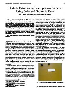
1. INTRODUCTION Once every year the Autonomous Unmanned Vehicle Society International holds a competition in which robots developed by Universities from around the world compete in a variety of challenging events. In the Ground Robotics Competition, robots must navigate a track made from painted lines on grass. The course contains obstacles such as 5 gallon buckets, construction barrels and simulated potholes. One of the largest challenges from this competition is creating the ability for the robot to stay inside the painted lines of the track and not get tricked or fooled by other visual items. Such items include white 5 gallon buckets, striped road construction barrels, white simulated pot holes, dashed and broken lines, ramps, simulated black top, variable distanced lines and a track with many curves. Add on top of this that the track is out doors and on rough grass then all of these things make following the lines of the track very difficult. Figure 1.0 gives a general idea of how the course looks.
1
Corrispondance: T. Nathan Mundhenk Michael Rivett Ernest L. Hall Center for Robotics Research
[email protected] [email protected] [email protected] http://www.robotics.uc.edu
Figure 1.0 This is how the track looked at the 2000 AUVSI ground robotics competition. Bearcat II is seen here entering simulated asphalt.
This paper discusses a variety of methods used by the University of Cincinnati’s Robotics Team to help the robot they designed, Bearcat II, navigate the course, distinguish between lines or other things and take appropriate actions when necessary. 1.1 Basic Line Following Techniques Bearcat II is equipped with two standard NTSC video cameras. Each camera is aimed toward the ground on either side of the robot. At any given moment, Bearcat II only tracks from one of the cameras. It tracks the lines by creating two windows sequentially. Each window is a section of the video picture. It then finds the centroid of the largest blob in that window. The centroid itself is formed by finding the most intense spots in the video window as determined by calibration of the tracking device, an ISCAN RK-446R automatic video tracker. The tracker returns to Bearcat’s computer the x and y position of the centroid as well as its size in height and width. This is done for each of the two windows. The coordinates from the ISCAN are then converted into real world coordinates via a transformation matrix [1]. The two points are then connected and the angle and distance can be estimated with great accuracy. Figure 1.1 shows a layout of how this tracking works
Figure 1.1 This is a representation of the view through the camera and how the ISCAN tracker and computer discover the track line by using a line of best fit approach
The robot then takes such data and will turn itself to be inline parallel with the line it is tracking. In order to stay towards the middle of the track, Bearcat will modify its course by adding a correction based upon how close it is to the line. At the ideal distance, usually in the middle of the track, this modifier is 0. As Bearcat approaches the line this number grows to the maximum correction set by the developer. The ISCAN tracker can also fulfill another role. When it loses track of the line, that is, when it can no longer find a centroid, it reports a loss of track. This can be very helpful since the lines on either of the tracks can be broken and the robot will need to know when to switch the camera to track the other side of the track. When it needs to do this, the computer sends a signal to a video switch, which switches the cameras. 1.2 Problems with this system This simple system is not without its limitations. The first such problem arises such that the robot will only switch cameras for a complete loss of track. The track is on grass. Grass itself is smooth and erratically reflective. It is easy for the robot to find a spot of higher intensity to track. A single shiny blade of grass is all that’s required. When the line is lost, the robot may track a blade of grass instead. As such, its course will be incorrect and possibly catastrophic. Another major problem encountered with this system is that objects are frequently encountered on the track that are more attractive targets than the line. Items such as white five gallon buckets and orange constructions barrels with white stripes are intentionally placed on the course in part for just such a purpose. The end result is that the robot may track the five-gallon bucket instead of the line. The course the robot then sets upon is incorrect and may either steer the robot away from the line, or into the line. Figure 1.2 shows how a bucket in the path of one window can cause the robot to misread the line.
Figure 1.2 A five gallon bucket or another object can distort the line of best fit and cause the robot to get an incorrect reading of the line. The results can be catastrophic.
In addition to the things that are placed on the track to trick the robot, other things wind up on the track inadvertently that can also trick the it. Such things include, but are not limited to, shadows and patches of dirt. Shadows can act negatively on the robots system by causing the intensity of the line to change suddenly. The ISCAN tracker will attempt to adjust to such things, but may do so incorrectly. The end result may be an incorrect or lost track. Dirt may also present itself as a challenge. The grass on the test track at the University of Cincinnati was filled with bald patches from the heavy student traffic. The dirt in the region is very light colored when dry. As a result, in sunlight it can appear very intense to the ISCAN tracker. The dirt patches can be a great problem because they can be anywhere and any size. As a result, a very rough lawn can be very difficult for the robot to navigate.
2. SOLUTIONS A number of solutions were implemented to attempt to solve these problems. These include statistically based expectancy systems and simple heuristic systems. These systems were implemented simultaneously and helped the robot to discriminate between what is a line on the track and what is something else. When it was able to discriminate the robot then had to decide what action to take. 2.1 Adaptive Line Discrimination Statistical Array One of the first lines of detection for the discrimination system was to build an array of predetermined size that included the width of the last n measurements of the line. For instance, this was commonly set to five. The robot would then add a good measurement to this array of five elements. When another measurement was taken it would then be compared to this array. If the new measurement was similar in size to the mean line size taken from the array, then that measurement was considered good and would then take its place on the array, bumping the oldest measurement. If the width of the line was too
small it would not be added, but could still be passed to the next stage as long as it was not below a second threshold. If the line was to large, then the measurement was rejected and the window from which the measurement was taken was moved in an attempt to get a better reading. If that also failed then the line reading would be rejected and a loss of track would be sent to the computer. Figure 2.0 shows a simple flow chart for this logic.
Figure 2.0 This is the basic flow chart for the line discrimination array. This chart does not include the heuristic constant system or the angular discrimination mentioned later.
The robot then has the option of how to treat this loss of track. If the loss of track was on one window alone then the robot has the option of treating it as an anomaly. It would ignore the reading and set a straight course of 0°. If, on the other hand, the robot received a loss of track on both windows then the robot would switch to the camera to the other side. This way we are cautious about simply switching the camera since we in essence open our eye into a blind area. Further, when the camera is switched, the array
is reset. Each camera has its own array and when one camera is then blinded, it can no longer adapt to line changes. The key to this system is that the algorithm adapts to a changing line size. It also sets itself such that the first five readings it takes build the initial array. This has the effect of not needing a human to set the array prior to a track run by the robot. The things that do need to be set by the programmer are such things as array sizes and discrimination thresholds. The net effect of this system is to detect things that are to large or to small to be a line. A fivegallon bucket, large dirt patches and other such things are discriminated as not being lines. The robot then has an option as to how it wants to treat these things. A simple five-gallon bucket is small enough that simply moving the window to look around it is sufficient. A large patch of whitish dirt may be so vivid and persistent that only by switching to another camera may it avoid being tricked into tracking something that is not a line. 2.2 Heuristic Constants In addition to soft adaptive systems, hard heuristic constants are added. These are constants set by the programmer that reflect an absolute size, which is either far to big or to small to ever be a line. The advantage to such additions to the system is that it sets hard limits. The adaptive system can be fooled into increasing its size by a patch of dirt that gradually increases in size. This is but one example, and other things have been found to occasionally effect the adaptive system as well in such a manner. When something is found that is either to large or to small to be a line by the preset constant, it is treated the same as a line that is found to large by the adaptive array. The robot will attempt to move the window and get a new reading. Failing that, a loss of track is sent to the computer. If a loss of track is encountered in only one window then the robot will steer itself 0° forward. If it receives a loss of track for both windows then it will switch cameras. The ideal largest size for a line is the largest size that can be recorded for a good reading. This is the width that is recorded when the line lies diagonally across both windows as close to perpendicular to the robot as possible. Figure 2.1 shows what this would look like.
Figure 2.1 Laid diagonally as close to perpendicular as possible inside both windows yields the idea maximum width of the line
The smallest possible line threshold was obtained in this instance from observation and by monitoring the log files from a given run. Caution was needed since the line itself was small in the camera and varied quite a bit. By setting the smallest possible line we could avoid tracking bright grass blades and other small reflections. The result was a more honest report of a line when the lines are dashed. The robot could then use this constant to more accurately cope with the dashed and broken lines set up on the track during the contest. 2.3 Adaptive Angle Discrimination In addition to a line size discrimination system, a system was implemented to determine if the angle of the line is within expected parameters. An array of the last n angles of the line was kept. In this case the array was only three measurements in size. If a line was measured that had an angle from the robot that fell outside of expectancy then the robot would switch to another camera. The idea behind this system is to avoid accidentally mistaking an object for a line which is similarly sized as a line, but which is not a line. The system will compare the line angle to its array. This happens after the line discrimination methods are used and after the angle of the line is calculated. If the line is different from the other angles by too wide a margin then it treated as a problem of high concern. This is because unlike the line discrimination system which can switch the position of the windows, this system does not know which window is at fault. Therefore the robot chooses to switch cameras. The margin for detection is set high. The idea is not to catch all problems, but is instead designed to keep the robot from taking a sudden change in course. This is indeed one of the biggest problems with line-sized objects. Since they are small they may only be detected in one iteration. However, if the robot suddenly veers to one side it may run off the track before is has time to recover. The margin should be set with just such a scenario in mind.
3. RESULTS In the AUVSI competition, Bearcat II had its longest run of 180 feet along the track. This placed it 3rd and 5 feet behind 2nd placed University of Hosei from Japan. By the observation of the Cincinnati team, Bearcat had the longest run of any robot when the sun was not behind the clouds. This means that Bearcat had the longest run with shadows and reflections present. Bearcat did mostly what it was supposed to do. It ignored several five gallon buckets as well as several construction barrels. It also managed to deal properly with dashed lines. Bearcat managed to ignore two of the three simulated potholes, which are painted white. It was the only robot of the top three to miss all three potholes. Bearcat left the track on its longest run after being fooled by the third simulated pothole. Its actions showed it swerving around the pothole in a manner that indicated it had mistaken the pothole for a line. The results caused it to turn at a point when the track was curving in the opposite direction, which made it easier for it to run off the track. The results from the competition are printed in table 2.0. University - Robot Virginia Tech - ARTEMIS Hosei University - Amigo University of Cincinnati University of Colorado @ Denver Virginia Tech - Navigator Hosei University - Nectar 2000 Embry Riddle Aeronautical University University of Tulsa Michigan Tech Bluefield State College University of Alberta
Final Distance 232.5 ft 185.75 ft 180 ft 136.75 ft 125.33 ft 61.67 ft 60.33 ft 58.67 ft 26.5 ft 6.0 ft Unable to Compete
Devry Institute of Technology Trinity College Tennessee State University Oakland University
Unable to Compete Unable to Compete Unable to Compete Unable to Compete
Table 2.0 This is the final standing from the AUVSI Ground Robotics Competition’s Autonomous Challenge.
3.1 Discussion The system utilized is not without its problems. One of the major problems is with the complexity of the system. The programmer must understand each step in the algorithm very well in order to debug it. The flow chart shown earlier in figure 2.0 shows how one of the three systems works. It does not show its integration with the other two algorithms. Complexity is also increased because each window must have its own array. Each camera has two windows and thus, you have four arrays. The act of sewing this system together took some amount of work. Another problem with the system is that when a camera is switched, the arrays for the camera just activated must be rebuilt. This can come as a problem if the camera switches on over a five-gallon bucket. The new array will be flawed. This necessitates the careful use of camera switching. Too much switching may nullify the effectiveness of having an adaptive algorithm. The third problem with this system is that it requires some trial and error to derive optimal values for some of the algorithms. For instance, at what point in the adaptive line discrimination array is a measure significantly large enough to merit detected as a non-line? There are several variables such as this, which must be set. It however may be possible to set these in the future using a genetic algorithm to find more optimal values. Whether or not it would improve on the robots performance is unknown since the programmer may be able to arrive at more optimal values sooner than a genetic algorithm could in practice. The system does have several strengths as well. One such strength is the simplicity of the ideas behind the algorithm. It is important that others be able to understand how the robot makes the decisions that it does since the membership in the robotics team rotates frequently as team members graduate. While it may be difficult to code this system, at least the concepts behind it are simple.
4. CONCLUSIONS The systems described are viable and with work can continue to be improved. Bearcat’s excellent performance at the AUVSI Ground Robotics Competition showed that the systems work in practice, as Bearcat was able to ignore several vivid targets on the track. The system also showed its shortcomings as it was eventually tripped up by the third simulated pothole on the track.
5. REFERENCES [1] Sameer S. Parasnis, “Four Point Calibration and a Comparison of Optical Modeling and Neural Networks for Robot Guidance,” Masters Thesis, University of Cincinnati, 1999. [2] Ernest L. Hall, Computer Image Processing and Recognition, Academic Press, New York, 1979.