Simple supervised document geolocation with ... - ACL Anthology

Simple Supervised Document Geolocation with Geodesic Grids Benjamin P. Wing Department of Linguistics University of Texas at Austin Austin, TX 78712 USA [email protected]

Abstract We investigate automatic geolocation (i.e. identification of the location, expressed as latitude/longitude coordinates) of documents. Geolocation can be an effective means of summarizing large document collections and it is an important component of geographic information retrieval. We describe several simple supervised methods for document geolocation using only the document’s raw text as evidence. All of our methods predict locations in the context of geodesic grids of varying degrees of resolution. We evaluate the methods on geotagged Wikipedia articles and Twitter feeds. For Wikipedia, our best method obtains a median prediction error of just 11.8 kilometers. Twitter geolocation is more challenging: we obtain a median error of 479 km, an improvement on previous results for the dataset.

1 Introduction There are a variety of applications that arise from connecting linguistic content—be it a word, phrase, document, or entire corpus—to geography. Leidner (2008) provides a systematic overview of geography-based language applications over the previous decade, with a special focus on the problem of toponym resolution—identifying and disambiguating the references to locations in texts. Perhaps the most obvious and far-reaching application is geographic information retrieval (Ding et al., 2000; Martins, 2009; Andogah, 2010), with applications like MetaCarta’s geographic text search (Rauch et al., 2003) and NewsStand (Teitler et al., 2008); these allow users to browse and search for 955

Jason Baldridge Department of Linguistics University of Texas at Austin Austin, TX 78712 USA [email protected]

content through a geo-centric interface. The Perseus project performs automatic toponym resolution on historical texts in order to display a map with each text showing the locations that are mentioned (Smith and Crane, 2001); Google Books also does this for some books, though the toponyms are identified and resolved quite crudely. Hao et al (2010) use a location-based topic model to summarize travelogues, enrich them with automatically chosen images, and provide travel recommendations. Eisenstein et al (2010) investigate questions of dialectal differences and variation in regional interests in Twitter users using a collection of geotagged tweets. An intuitive and effective strategy for summarizing geographically-based data is identification of the location—a specific latitude and longitude—that forms the primary focus of each document. Determining a single location of a document is only a well-posed problem for certain documents, generally of fairly small size, but there are a number of natural situations in which such collections arise. For example, a great number of articles in Wikipedia have been manually geotagged; this allows those articles to appear in their geographic locations while geobrowsing in an application like Google Earth. Overell (2009) investigates the use of Wikipedia as a source of data for article geolocation, in addition to article classification by category (location, person, etc.) and toponym resolution. Overell’s main goal is toponym resolution, for which geolocation serves as an input feature. For document geolocation, Overell uses a simple model that makes use only of the metadata available (article title, incoming and outgoing links, etc.)—the actual article text

Proceedings of the 49th Annual Meeting of the Association for Computational Linguistics, pages 955–964, c Portland, Oregon, June 19-24, 2011. 2011 Association for Computational Linguistics

is not used at all. However, for many document collections, such metadata is unavailable, especially in the case of recently digitized historical documents. Eisenstein et al. (2010) evaluate their geographic topic model by geolocating USA-based Twitter users based on their tweet content. This is essentially a document geolocation task, where each document is a concatenation of all the tweets for a single user. Their geographic topic model receives supervision from many documents/users and predicts locations for unseen documents/users. In this paper, we tackle document geolocation using several simple supervised methods on the textual content of documents and a geodesic grid as a discrete representation of the earth’s surface. Our approach is similar to that of Serdyukov et al. (2009), who geolocate Flickr images using their associated textual tags.1 Essentially, the task is cast similarly to language modeling approaches in information retrieval (Ponte and Croft, 1998). Discrete cells representing areas on the earth’s surface correspond to documents (with each cell-document being a concatenation of all actual documents that are located in that cell); new documents are then geolocated to the most similar cell according to standard measures such as Kullback-Leibler divergence (Zhai and Lafferty, 2001). Performance is measured both on geotagged Wikipedia articles (Overell, 2009) and tweets (Eisenstein et al., 2010). We obtain high accuracy on Wikipedia using KL divergence, with a median error of just 11.8 kilometers. For the Twitter data set, we obtain a median error of 479 km, which improves on the 494 km error of Eisenstein et al. An advantage of our approach is that it is far simpler, is easy to implement, and scales straightforwardly to large datasets like Wikipedia.

2 Data Wikipedia As of April 15, 2011, Wikipedia has some 18.4 million content-bearing articles in 281 language-specific encyclopedias. Among these, 39 have over 100,000 articles, including 3.61 million articles in the English-language edition alone. Wikipedia articles generally cover a single subject; in addition, most articles that refer to geographically

fixed subjects are geotagged with their coordinates. Such articles are well-suited as a source of supervised content for document geolocation purposes. Furthermore, the existence of versions in multiple languages means that the techniques in this paper can easily be extended to cover documents written in many of the world’s most common languages. Wikipedia’s geotagged articles encompass more than just cities, geographic formations and landmarks. For example, articles for events (like the shooting of JFK) and vehicles (such as the frigate USS Constitution) are geotagged. The latter type of article is actually quite challenging to geolocate based on the text content: though the ship is moored in Boston, most of the page discusses its role in various battles along the eastern seaboard of the USA. However, such articles make up only a small fraction of the geotagged articles. For the experiments in this paper, we used a full dump of Wikipedia from September 4, 2010.2 Included in this dump is a total of 10,355,226 articles, of which 1,019,490 have been geotagged. Excluding various types of special-purpose articles used primarily for maintaining the site (specifically, redirect articles and articles outside the main namespace), the dump includes 3,431,722 content-bearing articles, of which 488,269 are geotagged. It is necessary to process the raw dump to obtain the plain text, as well as metadata such as geotagged coordinates. Extracting the coordinates, for example, is not a trivial task, as coordinates can be specified using multiple templates and in multiple formats. Automatically-processed versions of the English-language Wikipedia site are provided by Metaweb,3 which at first glance promised to significantly simplify the preprocessing. Unfortunately, these versions still need significant processing and they incorrectly eliminate some of the important metadata. In the end, we wrote our own code to process the raw dump. It should be possible to extend this code to handle other languages with little difficulty. See Lieberman and Lin (2009) for more discussion of a related effort to extract and use the geotagged articles in Wikipedia. The entire set of articles was split 80/10/10 in 2

1

We became aware of Serdyukov et al. (2009) during the writing of the camera-ready version of this paper.

956

http://download.wikimedia.org/enwiki/ 20100904/pages-articles.xml.bz2 3 http://download.freebase.com/wex/

round-robin fashion into training, development, and testing sets after randomizing the order of the articles, which preserved the proportion of geotagged articles. Running on the full data set is timeconsuming, so development was done on a subset of about 80,000 articles (19.9 million tokens) as a training set and 500 articles as a development set. Final evaluation was done on the full dataset, which includes 390,574 training articles (97.2 million tokens) and 48,589 test articles. A full run with all the six strategies described below (three baseline, three non-baseline) required about 4 months of computing time and about 10-16 GB of RAM when run on a 64bit Intel Xeon E5540 CPU; we completed such jobs in under two days (wall clock) using the Longhorn cluster at the Texas Advanced Computing Center. Geo-tagged Microblog Corpus As a second evaluation corpus on a different domain, we use the corpus of geotagged tweets collected and used by Eisenstein et al. (2010).4 It contains 380,000 messages from 9,500 users tweeting within the 48 states of the continental USA. We use the train/dev/test splits provided with the data; for these, the tweets of each user (a feed) have been concatenated to form a single document, and the location label associated with each document is the location of the first tweet by that user. This is generally a fair assumption as Twitter users typically tweet within a relatively small region. Given this setup, we will refer to Twitter users as documents in what follows; this keeps the terminology consistent with Wikipedia as well. The training split has 5,685 documents (1.58 million tokens). Replication Our code (part of the TextGrounder system), our processed version of Wikipedia, and instructions for replicating our experiments are available on the TextGrounder website.5

3 Grid representation for connecting texts to locations Geolocation involves identifying some spatial region with a unit of text—be it a word, phrase, or document. The earth’s surface is continuous, so a 4

http://www.ark.cs.cmu.edu/GeoText/ http://code.google.com/p/textgrounder/ wiki/WingBaldridge2011 5

957

natural approach is to predict locations using a continuous distribution. For example, Eisenstein et al. (2010) use Gaussian distributions to model the locations of Twitter users in the United States of America. This appears to work reasonably well for that restricted region, but is likely to run into problems when predicting locations for anywhere on earth— instead, spherical distributions like the von MisesFisher distribution would need to be employed. We take here the simpler alternative of discretizing the earth’s surface with a geodesic grid; this allows us to predict locations with a variety of standard approaches over discrete outcomes. There are many ways of constructing geodesic grids. Like Serdyukov et al. (2009), we use the simplest strategy: a grid of square cells of equal degree, such as 1◦ by 1◦ . This produces variable-size regions that shrink latitudinally, becoming progressively smaller and more elongated the closer they get towards the poles. Other strategies, such as the quaternary triangular mesh (Dutton, 1996), preserve equal area, but are considerably more complex to implement. Given that most of the populated regions of interest for us are closer to the equator than not and that we use cells of quite fine granularity (down to 0.05◦ ), the simple grid system was preferable. With such a discrete representation of the earth’s surface, there are four distributions that form the core of all our geolocation methods. The first is a standard multinomial distribution over the vocabulary for every cell in the grid. Given a grid G with cells ci and a vocabulary V with words wj , we have θci j = P (wj |ci ). The second distribution is the equivalent distribution for a single test document dk , i.e. θdk j = P (wj |dk ). The third distribution is the reverse of the first: for a given word, its distribution over the earth’s cells, κji = P (ci |wj ). The final distribution is over the cells, γi = P (ci ). This grid representation ignores all higher level regions, such as states, countries, rivers, and mountain ranges, but it is consistent with the geocoding in both the Wikipedia and Twitter datasets. Nonetheless, note that the κji for words referring to such regions is likely to be much flatter (spread out) but with most of the mass concentrated in a set of connected cells. Those for highly focused point-locations will jam up in a few disconnected cells—in the extreme case, toponyms like Spring-

field which are connected to many specific point locations around the earth. We use grids with cell sizes of varying granularity d×d for d = 0.1◦ , 0.5◦ , 1◦ , 5◦ , 10◦ . For example, with d=0.5◦ , a cell at the equator is roughly 56x55 km and at 45◦ latitude it is 39x55 km. At this resolution, there are a total of 259,200 cells, of which 35,750 are non-empty when using our Wikipedia training set. For comparison, at the equator a cell at d=5◦ is about 557x553 km (2,592 cells; 1,747 non-empty) and at d=0.1◦ a cell is about 11.3x10.6 km (6,480,000 cells; 170,005 non-empty). The geolocation methods predict a cell cˆ for a document, and the latitude and longitude of the degree-midpoint of the cell is used as the predicted location. Prediction error is the great-circle distance from these predicted locations to the locations given by the gold standard. The use of cell midpoints provides a fair comparison for predictions with different cell sizes. This differs from the evaluation metrics used by Serdyukov et al. (2009), which are all computed relative to a given grid size. With their metrics, results for different granularities cannot be directly compared because using larger cells means less ambiguity when choosing cˆ. With our distancebased evaluation, large cells are penalized by the distance from the midpoint to the actual location even when that location is in the same cell. Smaller cells reduce this penalty and permit the word distributions θci j to be much more specific for each cell, but they are harder to predict exactly and suffer more from sparse word counts compared to courser granularity. For large datasets like Wikipedia, fine-grained grids work very well, but the trade-off between resolution and sufficient training material shows up more clearly for the smaller Twitter dataset.

probability in a test document dk is:6 #(wj , dk ) θ˜dk j = P #(wl , dk ) wl ∈V

Similarly for a cell ci , we compute the unsmoothed word distribution by aggregating all of the documents located within ci : P

#(wj , dk ) dk ∈ci ˜ θci j = P P #(wl , dk )

4.1

Supervision

We acquire θ and κ straightforwardly from the training material. The unsmoothed estimate of word wj ’s 958

(2)

dk ∈ci wl ∈V

We compute the global distribution θDj over the set of all documents D in the same fashion. The word distribution of document dk backs off to the global distribution θDj . The probability mass αdk reserved for unseen words is determined by the empirical probability of having seen a word once in the document, motivated by Good-Turing smoothing. (The cell distributions are treated analogously.) That is:7

αdk =

|wj ∈ V s.t. #(wj , dk )=1| P #(wj , dk )

(3)

wj ∈V

(−dk )

θDj

=

1−

θDj P

θDl

(4)

wl ∈dk

θdk j

( (−d ) if θ˜dk j = 0 αdk θDj k , = (1−αdk )θ˜dk j , o.w.

(5)

The distributions over cells for each word simply renormalizes the θci j values to achieve a proper distribution:

4 Supervised models for document geolocation Our methods use only the text in the documents; predictions are made based on the distributions θ, κ, and ρ introduced in the previous section. No use is made of metadata, such as links/followers and infoboxes.

(1)

θc j κji = P i θci j

(6)

ci ∈G

A useful aspect of the κ distributions is that they can be plotted in a geobrowser using thematic mapping 6

We use #() to indicate the count of an event. is an adjusted version of θDj that is normalized over the subset of words not found in document dk . This adjustment ensures that the entire distribution is properly normalized. 7 (−dk ) θDj

techniques (Sandvik, 2008) to inspect the spread of a word over the earth. We used this as a simple way to verify the basic hypothesis that words that do not name locations are still useful for geolocation. Indeed, the Wikipedia distribution for mountain shows high density over the Rocky Mountains, Smokey Mountains, the Alps, and other ranges, while beach has high density in coastal areas. Words without inherent locational properties also have intuitively correct distributions: e.g., barbecue has high density over the south-eastern United States, Texas, Jamaica, and Australia, while wine is concentrated in France, Spain, Italy, Chile, Argentina, California, South Africa, and Australia.8 Finally, the cell distributions are simply the relative frequency of the number of documents in each |ci | . cell: γi = |D| A standard set of stop words are ignored. Also, all words are lowercased except in the case of the most-common-toponym baselines, where uppercase words serve as a fallback in case a toponym cannot be located in the article. 4.2

the test document is a good encoding for. With KL(θdk ||θci ), the log ratio of probabilities for each word is weighted by the probability of the word in θd j the test document, θdk j log θckj , which means that i the divergence is more sensitive to the document rather than the overall cell. As an example for why non-symmetric KL in this order is appropriate, consider geolocating a page in a densely geotagged cell, such as the page for the Washington Monument. The distribution of the cell containing the monument will represent the words from many other pages having to do with museums, US government, corporate buildings, and other nearby memorials and will have relatively small values for many of the words that are highly indicative of the monument’s location. Many of those words appear only once in the monument’s page, but this will still be a higher value than for the cell and will weight the contribution accordingly. Rather than computing KL(θdk ||θci ) over the entire vocabulary, we restrict it to only the words in the document to compute KL more efficiently:

Kullback-Leibler divergence

Given the distributions for each cell, θci , in the grid, we use an information retrieval approach to choose a location for a test document dk : compute the similarity between its word distribution θdk and that of each cell, and then choose the closest one. KullbackLeibler (KL) divergence is a natural choice for this (Zhai and Lafferty, 2001). For distribution P and Q, KL divergence is defined as: KL(P ||Q) =

X i

P (i) log

P (i) Q(i)

(7)

This quantity measures how good Q is as an encoding for P – the smaller it is the better. The best cell cˆKL is the one which provides the best encoding for the test document: cˆKL = arg min KL(θdk ||θci )

(8)

ci ∈G

KL(θdk ||θci ) =

X

θdk j log

wj ∈Vdk

θdk j θci j

(9)

Early experiments showed that it makes no difference in the outcome to include the rest of the vocabulary. Note that because θci is smoothed, there are no zeros, so this value is always defined. 4.3

Naive Bayes

Naive Bayes is a natural generative model for the task of choosing a cell, given the distributions θci and γ: to generate a document, choose a cell ci according to γ and then choose the words in the document according to θci :

cˆN B = arg max PN B (ci |dk ) ci ∈G

The fact that KL is not symmetric is desired here: the other direction, KL(θci ||θdk ), asks which cell 8

This also acts as an exploratory tool. For example, due to a big spike on Cebu Province in the Philippines we learned that Cebuanos take barbecue very, very seriously.

959

P (ci )P (dk |ci ) P (dk ) ci ∈G Y #(wj ,d ) k θci j = arg max γi = arg max

ci ∈G

wj ∈Vdk

(10)

1200 800 600 200

For each word, κji gives the probability of each cell in the grid. A simple way to compute a distribution for a document dk is to take a weighted average of the distributions for all words to compute the average cell probability (ACP):

mean error (km)

1000

Average cell probability

400

4.4

1400

This method maximizes the combination of the likelihood of the document P (dk |ci ) and the cell prior probability γi .

0

cˆACP = arg max PACP (ci |dk ) ci ∈G P #(wj , dk )κji

Most frequent toponym Avg. cell probability Naive Bayes Kullback−Leibler 0.1

0.5

wj ∈Vdk

= arg max P ci ∈G

= arg max ci ∈G

P

#(wj , dk )κjl

#(wj , dk )κji

10

(11)

wj ∈Vdk

This method, despite its conceptual simplicity, works well in practice. It could also be easily modified to use different weights for words, such as TF/IDF or relative frequency ratios between geolocated documents and non-geolocated documents, which we intend to try in future work. 4.5

5

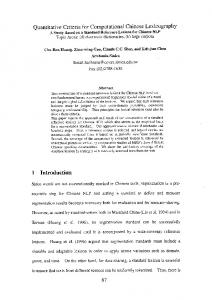
Figure 1: Plot of grid resolution in degrees versus mean error for each method on the Wikipedia dev set.

cl ∈G wj ∈Vdk

X

1 grid size (degrees)

Baselines

There are several natural baselines to use for comparison against the methods described above. Random Choose cˆrand randomly from a uniform distribution over the entire grid G. Cell prior maximum Choose the cell with the highest prior probability according to γ: cˆcpm = arg maxci ∈G γi . Most frequent toponym Identify the most frequent toponym in the article and the geotagged Wikipedia articles that match it. Then identify which of those articles has the most incoming links (a measure of its prominence), and then choose cˆmf t to be the cell that contains the geotagged location for that article. This is a strong baseline method, but can only be used with Wikipedia. Note that a toponym matches an article (or equivalently, the article is a candidate for the toponym) either if the toponym is the same as the article’s title, 960

or the same as the title after a parenthetical tag or comma-separated higher-level division is removed. For example, the toponym Tucson would match articles named Tucson, Tucson (city) or Tucson, Arizona. In this fashion, the set of toponyms, and the list of candidates for each toponym, is generated from the set of all geotagged Wikipedia articles.

5 Experiments The approaches described in the previous section are evaluated on both the geotagged Wikipedia and Twitter datasets. Given a predicted cell cˆ for a document, the prediction error is the great-circle distance between the true location and the center of cˆ, as described in section 3. Grid resolution and thresholding The major parameter of all our methods is the grid resolution. For both Wikipedia and Twitter, preliminary experiments on the development set were run to plot the prediction error for each method for each level of resolution, and the optimal resolution for each method was chosen for obtaining test results. For the Twitter dataset, an additional parameter is a threshold on the number of feeds each word occurs in: in the preprocessed splits of Eisenstein et al. (2010), all vocabulary items that appear in fewer than 40 feeds are ignored. This thresholding takes away a lot of very useful material; e.g. in the first feed, it removes

Thr. 0 2 3 5 10 20 40

0.1 1113.1 1018.5 1027.6 1011.7 1011.3 1032.5 1080.8

Grid size (degrees) 0.5 1 5 996.8 1005.1 969.3 959.5 944.6 911.2 940.8 954.0 913.6 951.0 954.2 892.0 968.8 938.5 929.8 987.3 966.0 940.0 1031.5 998.6 981.8

10 1052.5 1021.6 1026.2 1013.0 1048.0 1070.1 1127.8

Table 1: Mean prediction error (km) on the Twitter dev set for various combinations of vocabulary threshold (in feeds) and grid size, using the KL divergence strategy.

Figure 2: Histograms of distribution of error distances (in km) for grid size 0.5◦ for each method on the Wikipedia dev set.

both “kirkland” and “redmond” (towns in the Eastside of Lake Washington near Seattle), very useful information for geolocating that user. This suggests that a lower threshold would be better, and this is borne out by our experiments. Figure 1 graphs the mean error of each method for different resolutions on the Wikipedia dev set, and Figure 2 graphs the distribution of error distances for grid size 0.5◦ for each method on the Wikipedia dev set. These results indicate that a grid size even smaller than 0.1◦ might be beneficial. To test this, we ran experiments using a grid size of 0.05◦ and 0.01◦ using KL divergence. The mean errors on the dev set increased slightly, from 323 km to 348 and 329 km, respectively, indicating that 0.1◦ is indeed the minimum. For the Twitter dataset, we considered both grid size and vocabulary threshold. We recomputed the distributions using several values for both parameters and evaluated on the development set. Table 1 shows mean prediction error using KL divergence, for various combinations of threshold and grid size. Similar tables were constructed for the other strategies. Clearly, the larger grid size of 5◦ is more optimal than the 0.1◦ best for Wikipedia. This is unsurprising, given the small size of the corpus. Overall, there is a less clear trend for the other methods 961

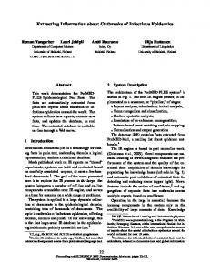
in terms of optimal resolution. Our interpretation of this is that there is greater sparsity for the Twitter dataset, and thus it is more sensitive to arbitrary aspects of how different user feeds are captured in different cells at different granularities. For the non-baseline strategies, a threshold between about 2 and 5 was best, although no one value in this range was clearly better than another. Results Based on the optimal resolutions for each method, Table 2 provides the median and mean errors of the methods for both datasets, when run on the test sets. The results clearly show that KL divergence does the best of all the methods considered, with Naive Bayes a close second. Prediction on Wikipedia is very good, with a median value of 11.8 km. Error on Twitter is much higher at 479 km. Nonetheless, this beats Eisenstein et al.’s (2010) median results, though our mean is worse at 967. Using the same threshold of 40 as Eisenstein et al., our results using KL divergence are slightly worse than theirs: median error of 516 km and mean of 986 km. The difference between Wikipedia and Twitter is unsurprising for several reasons. Wikipedia articles tend to use a lot of toponyms and words that correlate strongly with particular places while many, perhaps most, tweets discuss quotidian details such as what the user ate for lunch. Second, Wikipedia articles are generally longer and thus provide more text to base predictions on. Finally, there are orders of magnitude more training examples for Wikipedia, which allows for greater grid resolution and thus more precise location predictions.

Strategy Kullback-Leibler Naive Bayes Avg. cell probability Most frequent toponym Cell prior maximum Random Eisenstein et al.

Wikipedia Degree Median Mean 0.1 11.8 221 0.1 15.5 314 0.1 24.1 1421 0.5 136 1927 5 2333 4309 0.1 7259 7192 -

Threshold 5 5 2 N/A 20 40

Twitter Degree Median 5 479 5 528 10 659 0.1 726 0.1 1217 N/A 494

Mean 967 989 1184 1141 1588 900

Table 2: Prediction error (km) on the Wikipedia and Twitter test sets for each of the strategies using the optimal grid resolution and (for Twitter) the optimal threshold, as determined by performance on the corresponding development sets. Eisenstein et al. (2010) used a fixed Twitter threshold of 40. Threshold makes no difference for cell prior maximum.

Ships One of the most difficult types of Wikipedia pages to disambiguate are those of ships that either are stored or had sunk at a particular location. These articles tend to discuss the exploits of these ships, not their final resting places. Location error on these is usually quite large. However, prediction is quite good for ships that were sunk in particular battles which are described in detail on the page; examples are the USS Gambier Bay, USS Hammann (DD412), and the HMS Majestic (1895). Another situation that gives good results is when a ship is retired in a location where it is a prominent feature and is thus mentioned in the training set at that location. An example is the USS Turner Joy, which is in Bremerton, Washington and figures prominently in the page for Bremerton (which is in the training set). Another interesting aspect of geolocating ship articles is that ships tend to end up sunk in remote battle locations, such that their article is the only one located in the cell covering the location in the training set. Ship terminology thus dominates such cells, with the effect that our models often (incorrectly) geolocate test articles about other ships to such locations (and often about ships with similar properties). This also leads to generally more accurate geolocation of HMS ships over USS ships; the former seem to have been sunk in more concentrated regions that are themselves less spread out globally.

6 Related work Lieberman and Lin (2009) also work with geotagged Wikipedia articles, but they do in order so to ana962

lyze the likely locations of users who edit such articles. Other researchers have investigated the use of Wikipedia as a source of data for other supervised NLP tasks. Mihalcea and colleagues have investigated the use of Wikipedia in conjunction with word sense disambiguation (Mihalcea, 2007), keyword extraction and linking (Mihalcea and Csomai, 2007) and topic identification (Coursey et al., 2009; Coursey and Mihalcea, 2009). Cucerzan (2007) used Wikipedia to do named entity disambiguation, i.e. identification and coreferencing of named entities by linking them to the Wikipedia article describing the entity. Some approaches to document geolocation rely largely or entirely on non-textual metadata, which is often unavailable for many corpora of interest, Nonetheless, our methods could be combined with such methods when such metadata is available. For example, given that both Wikipedia and Twitter have a linked structure between documents, it would be possible to use the link-based method given in Backstrom et al. (2010) for predicting the location of Facebook users based on their friends’ locations. It is possible that combining their approach with our text-based approach would provide improvements for Facebook, Twitter and Wikipedia datasets. For example, their method performs poorly for users with few geolocated friends, but results improved by combining link-based predictions with IP address predictions. The text written users’ updates could be an additional aid for locating such users.

7 Conclusion We have shown that automatic identification of the location of a document based only on its text can be performed with high accuracy using simple supervised methods and a discrete grid representation of the earth’s surface. All of our methods are simple to implement, and both training and testing can be easily parallelized. Our most effective geolocation strategy finds the grid cell whose word distribution has the smallest KL divergence from that of the test document, and easily beats several effective baselines. We predict the location of Wikipedia pages to a median error of 11.8 km and mean error of 221 km. For Twitter, we obtain a median error of 479 km and mean error of 967 km. Using naive Bayes and a simple averaging of word-level cell distributions also both worked well; however, KL was more effective, we believe, because it weights the words in the document most heavily, and thus puts less importance on the less specific word distributions of each cell. Though we only use text, link-based predictions using the follower graph, as Backstrom et al. (2010) do for Facebook, could improve results on the Twitter task considered here. It could also help with Wikipedia, especially for buildings: for example, the page for Independence Hall in Philadelphia links to geotagged “friend” pages for Philadelphia, the Liberty Bell, and many other nearby locations and buildings. However, we note that we are still primarily interested in geolocation with only text because there are a great many situations in which such linked structure is unavailable. This is especially true for historical corpora like those made available by the Perseus project.9 The task of identifying a single location for an entire document provides a convenient way of evaluating approaches for connecting texts with locations, but it is not fully coherent in the context of documents that cover multiple locations. Nonetheless, both the average cell probability and naive Bayes models output a distribution over all cells, which could be used to assign multiple locations. Furthermore, these cell distributions could additionally be used to define a document level prior for resolution of individual toponyms. 9

www.perseus.tufts.edu/

963

Though we treated the grid resolution as a parameter, the grids themselves form a hierarchy of cells containing finer-grained cells. Given this, there are a number of obvious ways to combine predictions from different resolutions. For example, given a cell of the finest grain, the average cell probability and naive Bayes models could successively back off to the values produced by their coarser-grained containing cells, and KL divergence could be summed from finest-to-coarsest grain. Another strategy for making models less sensitive to grid resolution is to smooth the per-cell word distributions over neighboring cells; this strategy improved results on Flickr photo geolocation for Serdyukov et al. (2009). An additional area to explore is to remove the bag-of-words assumption and take into account the ordering between words. This should have a number of obvious benefits, among which are sensitivity to multi-word toponyms such as New York, collocations such as London, Ontario or London in Ontario, and highly indicative terms such as egg cream that are made up of generic constituents.

Acknowledgments This research was supported by a grant from the Morris Memorial Trust Fund of the New York Community Trust and from the Longhorn Innovation Fund for Technology. This paper benefited from reviewer comments and from discussion in the Natural Language Learning reading group at UT Austin, with particular thanks to Matt Lease.

References Geoffrey Andogah. 2010. Geographically Constrained Information Retrieval. Ph.D. thesis, University of Groningen, Groningen, Netherlands, May. Lars Backstrom, Eric Sun, and Cameron Marlow. 2010. Find me if you can: improving geographical prediction with social and spatial proximity. In Proceedings of the 19th international conference on World wide web, WWW ’10, pages 61–70, New York, NY, USA. ACM. Kino Coursey and Rada Mihalcea. 2009. Topic identification using wikipedia graph centrality. In Proceedings of Human Language Technologies: The 2009 Annual Conference of the North American Chapter of the Association for Computational Linguistics, Companion Volume: Short Papers, NAACL ’09, pages 117–

120, Morristown, NJ, USA. Association for Computational Linguistics. Kino Coursey, Rada Mihalcea, and William Moen. 2009. Using encyclopedic knowledge for automatic topic identification. In Proceedings of the Thirteenth Conference on Computational Natural Language Learning, CoNLL ’09, pages 210–218, Morristown, NJ, USA. Association for Computational Linguistics. Silviu Cucerzan. 2007. Large-scale named entity disambiguation based on Wikipedia data. In Proceedings of the 2007 Joint Conference on Empirical Methods in Natural Language Processing and Computational Natural Language Learning (EMNLP-CoNLL), pages 708–716, Prague, Czech Republic, June. Association for Computational Linguistics. Junyan Ding, Luis Gravano, and Narayanan Shivakumar. 2000. Computing geographical scopes of web resources. In Proceedings of the 26th International Conference on Very Large Data Bases, VLDB ’00, pages 545–556, San Francisco, CA, USA. Morgan Kaufmann Publishers Inc. G. Dutton. 1996. Encoding and handling geospatial data with hierarchical triangular meshes. In M.J. Kraak and M. Molenaar, editors, Advances in GIS Research II, pages 505–518, London. Taylor and Francis. Jacob Eisenstein, Brendan O’Connor, Noah A. Smith, and Eric P. Xing. 2010. A latent variable model for geographic lexical variation. In Proceedings of the 2010 Conference on Empirical Methods in Natural Language Processing, pages 1277–1287, Cambridge, MA, October. Association for Computational Linguistics. Qiang Hao, Rui Cai, Changhu Wang, Rong Xiao, JiangMing Yang, Yanwei Pang, and Lei Zhang. 2010. Equip tourists with knowledge mined from travelogues. In Proceedings of the 19th international conference on World wide web, WWW ’10, pages 401– 410, New York, NY, USA. ACM. Jochen L. Leidner. 2008. Toponym Resolution in Text: Annotation, Evaluation and Applications of Spatial Grounding of Place Names. Dissertation.Com, January. M. D. Lieberman and J. Lin. 2009. You are where you edit: Locating Wikipedia users through edit histories. In ICWSM’09: Proceedings of the 3rd International AAAI Conference on Weblogs and Social Media, pages 106–113, San Jose, CA, May. Bruno Martins. 2009. Geographically Aware Web Text Mining. Ph.D. thesis, University of Lisbon. Rada Mihalcea and Andras Csomai. 2007. Wikify!: linking documents to encyclopedic knowledge. In Proceedings of the sixteenth ACM conference on Conference on information and knowledge management,

964

CIKM ’07, pages 233–242, New York, NY, USA. ACM. Rada Mihalcea. 2007. Using Wikipedia for Automatic Word Sense Disambiguation. In North American Chapter of the Association for Computational Linguistics (NAACL 2007). Simon Overell. 2009. Geographic Information Retrieval: Classification, Disambiguation and Modelling. Ph.D. thesis, Imperial College London. Jay M. Ponte and W. Bruce Croft. 1998. A language modeling approach to information retrieval. In Proceedings of the 21st annual international ACM SIGIR conference on Research and development in information retrieval, SIGIR ’98, pages 275–281, New York, NY, USA. ACM. Erik Rauch, Michael Bukatin, and Kenneth Baker. 2003. A confidence-based framework for disambiguating geographic terms. In Proceedings of the HLT-NAACL 2003 workshop on Analysis of geographic references - Volume 1, HLT-NAACL-GEOREF ’03, pages 50–54, Stroudsburg, PA, USA. Association for Computational Linguistics. Bjorn Sandvik. 2008. Using KML for thematic mapping. Master’s thesis, The University of Edinburgh. Pavel Serdyukov, Vanessa Murdock, and Roelof van Zwol. 2009. Placing flickr photos on a map. In Proceedings of the 32nd international ACM SIGIR conference on Research and development in information retrieval, SIGIR ’09, pages 484–491, New York, NY, USA. ACM. David A. Smith and Gregory Crane. 2001. Disambiguating geographic names in a historical digital library. In Proceedings of the 5th European Conference on Research and Advanced Technology for Digital Libraries, ECDL ’01, pages 127–136, London, UK. Springer-Verlag. B. E. Teitler, M. D. Lieberman, D. Panozzo, J. Sankaranarayanan, H. Samet, and J. Sperling. 2008. NewsStand: A new view on news. In GIS’08: Proceedings of the 16th ACM SIGSPATIAL International Conference on Advances in Geographic Information Systems, pages 144–153, Irvine, CA, November. Chengxiang Zhai and John Lafferty. 2001. Model-based feedback in the language modeling approach to information retrieval. In Proceedings of the tenth international conference on Information and knowledge management, CIKM ’01, pages 403–410, New York, NY, USA. ACM.