simulated annealing for materialized view selection in data ...

SIMULATED ANNEALING FOR MATERIALIZED VIEW SELECTION IN DATA WAREHOUSING ENVIRONMENT Roozbeh Derakhshan 1 1

Frank Dehne 2

Othmar Korn 1

Bela Stantic 1

Institute for Integrated and Intelligent Systems Griffith University, Brisbane, Australia 2 School of Computer Science Carleton University, Canada

ABSTRACT In order to facilitate query processing, the information contained in data warehouses is typically stored as a set of materialized views. Deciding which views to materialize presents a considerable challenge. The task is to select from a very large search space a set of views that minimizes view maintenance and query processing costs. Heuristic methods have been employed to find near optimal solutions and recent genetic algorithms have significantly improved the quality of the obtained solutions. In this paper we introduce a new approach for materialized view selection that is based on Simulated Annealing in conjunction with the use of a Multiple View Processing Plan (MVPP). Our experiments show that our new method provides a further significant improvement in the quality of the obtained set of materialized views, leading to a further significant improvement in query processing time and view maintenance costs for data warehousing systems. KEY WORDS Data warehousing, materialized view selection, query optimization, simulated annealing

1 Introduction Data warehouses integrate data from multiple, distributed, heterogeneous databases and other information sources. Information within a data warehouse is organized as a set of views from different production databases. These views are often referred to as materialized views. The large computation and space required for view materialization implies that it is impractical to materialize all possible views. Hence, there is a need for selecting an appropriate set of views to materialize that strikes a balance between computational cost and increased query performance, commonly referred to as the ”view selection problem” [4]. The task is to select a set of views that minimizes view maintenance and query processing costs. The view selection problem is NP-complete. Several heuristic methods have been proposed in the literature to address the view selection problem such as [4],[5], [5],[7], [1],[2] and [11]. In [12] a ”chunk” based precomputation

method was introduced. This method precomputes a subset of chunk aggregates which provide better but not near optimal results over the heuristic approaches. In order to obtain better solutions with respect to view maintenance and query processing costs, evolutionary approaches (genetic algorithms) have recently been proposed [15, 16], [9], [8]. However, the possibility of infeasible solutions creates some problems. In fact, the approach in [15, 16] does not contain a ”penalty” method to discourage infeasible solutions. This deficiency has subsequently been addressed in [9]. However, the experimental evaluation of [9] with respect to view maintenance and query processing costs was performed only for very small (unrealistic) data sets. Subsequently method was improved by adding of a penalty function, but tests were performed on only twenty views and eight dimensions, which is unrealistically small problem size to prove dominance of the approach [9]. The best evolutionary approach in terms of completeness of methodology, performance evaluation, and quality of the results was published in [8]. It provides experimental results which show that the cost of their reported sets of selected views is considerably better than than the previously reported heuristics. In this paper we introduce a new approach for materialized view selection that is based on Simulated Annealing (SA) in conjunction with the use of a Multiple View Processing Plan (MVPP)[7]. In experimental study we show that, compared to [8], our method provides a further significant improvement in the quality of the obtained set of materialized views, leading to a further significant improvement in query processing time and view maintenance costs for data warehousing systems. Furthermore, our method does not rely on penalty functions which can still lead to infeasible solutions in rare cases. Instead, our method guarantees that the reported solution is feasible, i.e. contains the views required to answer queries, by adding a constraint to our SA algorithm that checks the feasibility of the solution against the number of queries that each solution can answer. In the following Section 2, we review the materialized view selection problem and the Multiple View Processing Plan (MVPP)[7]. In Section 3 we discuss our Simulated

need to consider data communication costs in our cost calculation. Suppose that we have the following frequently used queries:

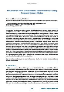
Figure 1. Basic Architecture of Data Warehousing

Annealing approach and how we apply SA to solve materialized view selection. Section 4 describes our experimental results, and Section 5 concludes the paper.

2 Background Materialized view selection is an important design decision in data warehouse construction. Figure 1 illustrates the basic architecture of a data warehouse [10]. The information sources store historical information. Each information source connects to a wrapper/monitor that is responsible for data translation and change detection. The wrapper translates the source schema to the schema utilized by the data warehouse, and the monitor detects changes in the source which are then passed on to the integrator. The integrator is responsible for the insertion and modification of information within the data warehouse, dispersing changes in source relations and maintaining tables in the warehouse as required.

2.1 Running Example In this section, we present an example to motivate the discussion of materialized view selection in data warehouse. Our example is taken from a sample data warehouse application which analyzes trends in sales, and which was used in [14]. The relations and the attributes of our example’s schema are: Product (Pid, name, Did) Division (Did, name, city) Order(Pid,Cid, quantity, date) Customer (Cid, name, city) Part (Tid, name, Pid, supplier) We use Pd, Div, Ord, Cust and Pt to refer ro the above relations. Furthermore, we assume that all of these relations are stored at the same site and we do not

Query 1:

Select Pd.name From Pd, Div Where Div.city= "LA" and Pd.Did=Div.Did

Query 2:

Select Pt.name From Pd, Pt, Div Where Div.city="LA" and Pd.Did=Div.Did and Pt.Pid=Pd.Pid

Query 3:

Select Cust.city, date From Ord, Cust Where quantity>100 and Ord.Cid=Cust.Cid

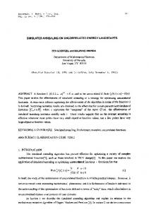
Figure 2 represents a global query access plan for the above four queries. This plan is referred to as Multiple View Processing Plan (MVPP) [7]. The query access frequencies are indicated above each query node. For simplicity, we assumed that the base relations Pd, Div, Ord, Cust, and Pt are updated once during the process of materialized view selection. We have different options for selection of a set of views to be materialized: (1) materialize all of the nodes in the MVPP; (2) materialize some of the intermediate nodes (e.g. tmp2, tmp3, tmp7, etc.); (3) do not materialize any of the nodes in MVPP. Option (1) and (3) are not realistic because for option (1), we do not have enough time and space to materialized all of the nodes in MVPP. Option (3) implies that we have to execute all queries on the raw data set, which will result in excessive query processing times. The best option is to materialize an appropriate subset of views that minimizes view maintenance and query processing costs. Suppose there are some materialized intermediate nodes in the MVPP. For each query, the cost of query processing is its query frequencies multiplied by the cost of the query accesses to the materialized nodes. The maintenance cost for materialized view is the cost used for construction of this view (here we assume that rebuilding is used whenever an update of an involved base relation occurs) [7]. For example, if tmp2 is materialized, the query processing cost for Q1 is 10 ∗ 35.25. The view maintenance cost is 2 ∗ (35.25 + 0.25). The total cost for an MVPP is the sum of all query processing and view maintenance costs. What follows is a specification and the definition of the cost model for a MVPP.

2.2

Review of the Multiple View Processing Plan (MVPP)

We intend to use a MVPP [7] together with Simulated Annealing for selecting the best set of views to materialize.

As shown in Figure 2, the MVPP is a directed acyclic graph (DAG) that represents a query processing plan for a data warehouse. The leaf nodes in this graph represent the base relations, and the root nodes represent the queries. Analogous to query execution plans there can be more than one MVPP for the same set of views. This depends upon the access characteristics of the applications and physical data warehouse parameters. We choose one of the possible optimal MVPPs. Note that, the quality of the selected MVPP can effect on our result. An MVPP is a dag r M = (V, A, Cqa , Cm , fq , fu ) where V is a set of vertices, A is a set of arcs over V defined as follows: • For every relational algebra operation in the query tree, for every base relation, and for every distinct query, create a vertex; • For v ∈ V, T (v) is the relation generated by the corresponding vertex v. T (v) can be a base relation, intermediate node while processing a query, or the final result for a query; • For any leaf vertex v, (that is one which has no edges pointing to the vertex), T (v) corresponds to a base relation. Let L be a set of leaf nodes; • For any root vertex v (that is one which has no edges going out of the vertex), T (v) corresponds to a global query. Let R be a set of root nodes; • If the base relation or intermediate result relation T (u) corresponding to vertex u is needed for further processing at a node v, introduce an arc u −→ v; • For every vertex v, let S(v) denote the source nodes which have edges pointed to v; for any v ∈ L,S(v) = φ, S ∗ (v) be the set of descendants of v; • For every vertex v let D(v) denote the destination nodes to which v is is pointed; for any v ∈ R , D(v) = φ; • For v ∈ V ,Cqa is the cost of query processing q acr cessing T (v); Cm (v) is the cost of maintaining T (v) based on changes to the base relation S ∗ (v) ∩ R , if T (v) is materialized. • fq , fu denote query frequency and base relation maintenance frequency respectively.

2.3

Cost Model

We can now define the cost function for our problem, similar to the cost function defined in [7]. The cost function has two parts, one is the query processing cost: Cqueryprocessing (v) = Σq∈R fq Caq (v) The second part is the materialized view maintenance cost: r Cmaintenance (v) = Σr∈R fu Cm (v)

. The total cost is the sum of query processing cost and maintenance cost: Ctotal (v) = Cqueryprocessing (v) + Cmaintenance (v) Our goal is to find the set of views so that if the members of the set are materialized then the value of Ctotal will be smallest among all the possible feasible sets of materialized views.

3

Our Approach: Simulated Annealing for Materialized View Selection

Our approach uses a Simulated Annealing (SA) algorithm. The motivation to use a SA algorithm in solving the materialized view selection problem was based on the observation that a data warehouse can have a huge number of views and the queries and may change frequently. Thus, materialized view selection is considered a complex problem with a very large state space. Metaheuristic methods, such as SA, try to find the global minimum by traversing only parts of the sate space [6]. However, the success and quality of the SA algorithms relies on choosing the right parameters such as proper problem specification, setting-up of the algorithm and also fine-tuning of the algorithm during many test runs. In the following subsections, we give a brief review of SA and provide details on how to apply SA to design a solution for the materialized view selection problem. More precisely, we provide a suitable representation of the solution space as well as some of the important parameters in the SA algorithm.

3.1

Simulated Annealing Framework

Simulated annealing (SA) is a flexible optimization method that is suited for large combinatorial optimization problems. SA has been applied successfully for many combinatorial optimization problems such as Travelling Salesman Problem (TSP). SA method is useful for problems that are characterized with a very large discrete configuration space, which is too large for an exhaustive search, over which an objective cost function is to be minimized (or maximized) [10]. After choosing the initial configuration, most iterative methods continue by choosing a new configuration at each step, evaluating it and possibly replacing the previous one with it. This action is repeated until some termination condition is satisfied. The procedure ends in a minimum configuration (based on the cost function), but generally it is a local minimum rather than the desired global minimum. The SA method tries to escape from these local minima by using some random moves, the frequencies of these moves depends on the temperature T . The following are some important parameters that must be determined when we use the SA method: • Set of initial configuration which is normally created randomly.

Figure 2. A MVPP for example queries

• Generation of new configuration by perturbing the existing configuration.

3.2

Solution Representation

• Choose a new configuration S0 in the neighborhood of S;

The problem to be solved can be stated as follows: given a MVPP graph (see figure 2) we attempt to find the best set of intermediate nodes (views) that can answer all queries with minimal cost. We do not use an MVPP directly as input into our SA algorithm. We first convert the set of views to a binary string of 1s and 0s to represent views that will and will not be materialized, respectively. Our mapping strategy differs from [15],[16] and [9]. We number our nodes starting at the base relations moving left to right, and we continue up to the right-most node at the top of the graph. Nodes are numbered 0 to m - 1 (where m is the number of intermediate nodes). We use a mapping array of size m-1 where each index in the array corresponds to a graph node. In our mapping array ’1’ denotes that the corresponding node in the graph should be materialized and ’0’ associate that the node is not materialized. For example, in the binary string (0,0,0,0,1,1,0,0,1,1,0) nodes 4,5,8 and 9 are materialized.

• Let E and E0 be the values of the cost function at S and S0, respectively; if E0 < E or random < e(E−E0)/T then set S←−S0;

3.3

• Cost function to be minimize over the configurations. • Cooling schedule, including the initial temperature and how and when to decrease it. • Termination condition. Now, an abstract view of the SA is listed in the below: The algorithm proceeds as follows[10]: 1. Choose an initial configuration s and an initial temperature T ; 2. Repeat the following (usually some fixed number of times):

3. Decrease the temperature T ; 4. If the termination rule is satisfied, stop; otherwise go back to Step 2. What follows is a description how this algorithm can be adapted to solve the materialized selection problem.

Simulated Annealing Parameters

The success of Simulated Annealing is dependant on certain parameters, as mentioned in section 3.1. Although, some parameters are problem independent [6] others remain implementation specific, such as initial configuration, random configuration perturbation and cost function. • Initial configuration: In our initial configuration we

map array with a randomized set of zeros and ones. We do not employ a penalty function to discourage infeasible solutions, instead we use a simple verification method. We check the feasibility of each initial configuration against the number of queries that the solution can answer. If the solution is not feasible, we simply bypass it. For example the sequence (0,0,0,1,1,0,0,0,0,0,0) is a feasible solution for our sample problem. In figure 2 the materialized node 3 can answer queries 1 to 3 and materialized node 4 answers the 4th query. • Perturbing the configuration: In the spirit of the physical annealing process, neighboring configurations must be similar in the sense that they represent only a slight perturbation in the system’s state [10]. Consequently, we define the neighborhood of a configuration to contain all configurations that differ from it by the removal of a single node. That is, we remove a randomly chosen node from the existing configuration in each run. We continue to remove nodes from the configuration until we reach the run length limit or until we reach an infeasible solution. By doing that, each time the new configuration can create a new set of views which can answer the queries with a lower cost than previous configurations. • Cost function: We use the cost function described in section 2.3. For example, to calculate the overall cost for the solution (0,0,0,1,1,0,0,0,0,0,0) we add Ctotal for nodes 3 and 4.

4

Experimental Evaluation

We have implemented simulated annealing for materialized view selection using an existing simulated annealing package [3]. We combined this with our problem definition for materialized view selection described above. Simulated Annealing consists of a series of independent annealing runs of increasing length. The lowest cost encountered on each run is retained and the final reported result is the best cost over all runs. We need to set some implementationdependant simulated annealing parameters: starting temperature, starting chain length and cooling schedule. • Starting temperature: The temperature (T ) can affect the number and ratio of acceptance of each move. This value has traditionally been chosen so that nearly all moves are accepted. We set our starting temperature large enough to allow an acceptance value of 90. If the starting temperature is larger, run length may increase with no improvement in cost. Too low a temperature may lead to premature levelling off of the algorithm [3]. • Starting chain length: Our actual annealing starts with an initial chain length of 50. We discovered that this value performed well over many test runs and was sufficient to provide good results on early runs.

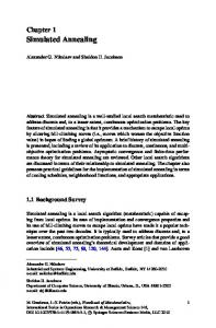
• Cooling schedule: The temperature decrement factor for the exponential cooling is set to a constant value of 0.7. This value performed sufficiently well on our problem, although the algorithm is not particularly sensitive to this parameter. Our experiment involves execution of our SA application over an optimized MVPP for 5 to 50 queries. Our SA application is a C program, which uses a robust SA library implementation [3] with the addition of our materialized view selection component. We executed our tests on an Intel Celeron 1.3GHz PC running Windows XP. The MVPP input is provided by our custom C++ MVPP builder, which creates an optimized MVPP given a set of SQL query inputs. We source fifty 8-dimensional input queries from the Transaction Processing Performance Council (TPC) [13] where individual query dimensions vary from 3 to 8. The number o nodes in our MVPP inputs varies from 22 to 250. Figure 3 compares our SA algorithm result to the evolutionary genetic algorithm and the heuristic algorithm for materialized view selection. The heuristic algorithm provides a benchmark for our normalized results. The graph shows that our SA algorithm approach generates solutions with costs up to 70% less than the genetic and heuristic algorithms. The relative improvements in cost are larger for a small number of queries and less for larger numbers of queries. However, due to the normalization in Figure 3, the improvement in cost for larger numbers of queries is more than it appear in the graph. The absolute values of the normalized costs for the Heuristic method increase dramatically with increasing number of queries. Hence, the absolute cost improvement provided by our method for larger numbers of queries is substantial.

5

Conclusion and Future work

In this paper we have introduced a new approach for materialized view selection based on Simulated Annealing. Compared to previous methods, our new method provides a significant improvement in the quality of the obtained set of materialized views. For large data warehousing systems, this leads to a significant improvement in query processing time and view maintenance costs. In the future, we plan to expand our approach to include parallel Simulated Annealing in order to deal with even larger sets of views and gain further improvements in solution quality.

6 Acknowledgements This research is partly sponsored by ARC (Australian Research Council) Discovery grant - Coarse Grained Parallel Algorithms, nr. DP0557303.

Figure 3. Experimental Results: Comparison of the solution quality (view maintenance and query processing costs) between Heuristic Method (normalized to ”1”), Genetic Algorithm [16], and Simulated Annealing (our approach).

References [1] E. Baralis, S.Paraboschi, and E.Teniente. Materialized view selection in a multidimensional database. Proceedings of the 23rd VLDB Conference, Athens, Greece, pages 156–165, 1997. [2] D.Theodoratos and T.Sellis. Data warehouse configuration. Proceedings of the 23rd VLDB Conference Athens, Greece,, pages 126–135, 1997. [3] G.S Stiles and Fu-Hsieng Lee . A ‘C’ Robust Simulated Annealing Package. http://www.engineering.usu.edu/ece/research/rtpc/ projects/comb/robust, 2003. [4] H. Gupta and I. S. Mumick. Selection of views to materialize under a maintenance cost constraint. Proceedings of the International Conference on Data Engineering, 1998. [5] V. Harinarayan, A. Rajaraman, and J. Ullman. Implementing data cubes efficiently. Proc. ACM SIGMOD Int’l Conf. Management Of Data, pages 205– 216, 1996. [6] Y. Ioannidis and E. Wong. Query optimization by simulated annealing. ACM SIGMOD International Conference on Management of Data,USA,San Francisco, pages 9–22, 1987. [7] J.Yang, K.Karlapalem, and Q.Li. Algorithm for materialized view design in data warehousing environment. Proceedings of the 23rd VLDB Conference, Athens, Greece, pages 136–145, 1997.

[8] X. Y. J.Yu, C.Choi, and G.Gou. Materialized view selection as constraint evolutionary optimization. IIEEE Trans, Sys, Man,Cybern, 33(4):485–467, 2003. [9] M. Lee and J. Hammer. Speeding up materialized view selection in data warehouses using a randomized rlgorithm. Int. J. Cooperative Inform. Syst., 10(3):327–353, 2001. [10] R.Davidson and D.Harel. Drawing graphs nicely using simulated annealing. ACM Transactions on Graphics, 15(4):301–331, 1996. [11] K. Ross, D.Srivastava, and S. Sudarshan. Materialized view maintenance and integrity constraint checking: Trading space for time. Proceedings ACM SIGMOD, pages 447–458, 1996. [12] A. Shukla, P. Deshpande, and J. Naughton. Materialized view selection of multidimensional datasets. Proceeding of the 24th VLDB Conference,New York,USA, pages 488–499, 1998. [13] Transaction Processing Performance Council. TPC benchmarks. http://www.tpc.org. [14] J. Yang, K.Karlapalem, and Q. Li. A framework for designing materialized views in data warehousing environment. Technical Report HKUST-CS96-35, 1996. [15] C. Zhang and J. Yang. Genetic algorithm for materialized view selection in data warehouse environments. Proc. Int’l Conf. Data Warehousing and Knowledge Discovery (DaWaK), pages 116–125, 1999. [16] C. Zhang, X. Yao, and J. Yang. An evolutionary Approach to Materialized View Selection In a Data Warehouse Environment. IEEE Trans. Syst., Man, Cybern, 31(3):282–293, 2001.