2003-01-2546
Simulating Advanced Life Support Systems for Integrated Controls Research David Kortenkamp Metrica Inc. at NASA Johnson Space Center ER2
Scott Bell S&K Technologies Inc. at NASA Johnson Space Center ER2 Copyright © 2003 SAE International
ABSTRACT This paper describes a simulation of an integrated advanced life support system. It contains models of the major components of an Advanced Life Support (ALS) system including crew, biomass, water recovery, air revitalization, food processing and power supply. The simulation also models malfunctions and stochastic processes. Sensors and actuators are modeled to allow controllers to interact with the simulation. The simulation is designed for testing and evaluation of life support control approaches. We use an example of a simple genetic algorithm to demonstrate how a control application might use the simulation. The simulation is implemented in Java to make it portable and easy to use.
INTRODUCTION
controlling advanced life support systems. For example is a distributed or hierarchical approach better? What role does machine learning play in control? How can symbolic, qualitative control approaches be integrated with continuous, quantitative approaches? How can we evaluate different control philosophies? The research in this paper does not answer these questions. Instead, it puts forth a mechanism by which we can begin to build systems which will provide us with answers. This paper starts with an overview of the models underlying the simulation. These models are taken from the best available simulations or hardware tests. We then discuss how external controllers can connect to the simulation. A simple external controller is implemented as a demonstration and some preliminary results are given. Finally, future directions for the simulation are discussed.
Advanced life support systems have multiple interacting subsystems which makes control a particularly challenging task. The simulation described in this paper provides a testbed for integrated control research. There have been other integrated life support simulations (e.g., [1]) and we have learned from those efforts. This simulation is designed exclusively for integrated controls research, which imposes different requirements. For example, the simulation is accessed through sensors and actuators, just as a real system would be. Noise and uncertainty are built in and controllable. Malfunctions and failures of subsystems are modeled and manifest themselves through anomalous readings in the sensors. Crew members are taskable and their tasks have purpose and meaning in the simulation. In essence, the simulation is a replacement for the Advanced Life Support (ALS) hardware and crew, allowing for testing of control approaches in advance of any integrated test.
SIMULATION OVERVIEW
We want the simulation to be used to develop and evaluate integrated control techniques. There are still many open research questions with respect to
The crew module is implemented using models described in [3]. The number, gender, age and weight of the crew are settable as input parameters – in the
A typical advanced life support system consists of multiple interacting modules [2]. We have modeled most of these modules using the best available information. The models are process models in that they take in certain resources and produce other resources. They are not component models, that is, they do not model physical objects such as valves, pumps, etc. We have designed our simulation to be completely configurable for the user. Any number of modules may be connected to any number of other modules. To ease the use for researchers unfamiliar with life support systems, we have a default configuration of modules. This default configuration is shown in Figure 1 and is described below. CREW MODULE
methane
vent
air RS
H2O
power
O2
air-in to all air-out CO2
crew environment air-in
activities
CO2 O2
O2 injector
injector
accum.
O2
air-out
crew
air-in
food
waste store
biomass
food processor
food store
action effects
solid waste
biomass environment
CO2
air-out
biomass
crop schedule
biomass store
solid waste
grey H2O
water RS waste RS dirty H2O
potable H2O
dirty H2O
potable H2O
grey H2O
Figure 1: The various modules that comprise the integrated simulation default configuration there are four crew members, two male and two female. The crew cycles through a set of activities (sleep, maintenance, recreation, etc.). As they do so they consume O2, food and water and produce CO2, dirty water and solid waste. The amount of resources consumed and produced varies according to crew member attributes and their activities. The crew’s activities can be adjusted by passing a new crew schedule to the crew module. A default schedule can also be used. The crew module is connected to a crew environment that contains an atmosphere that they breathe. The initial size and gas composition (percentages of O2, CO2, H2O and inert gases) are input parameters and the default size is 1.54893 x 10⁶liters (from [4]) with an atmosphere equivalent to sea level air. As the simulation progresses the composition of gases in the atmosphere changes. BIOMASS MODULE The biomass module models crops that produce food and oxygen in the simulation. Currently, only wheat crops are modeled, but we are adding eight additional crops in an upcoming release. The growing area of the
biomass module is fixed at the start of the simulation. Within this growing area the amounts of the different crops can be adjusted during a simulation run either through the crew interface or directly through the BioMass interface. As crops grow they consume CO2, potable or grey water and light. At the same time, they produce O2 and transpire H2O. The crops also produce biomass when they are harvested. The production and consumption of resources are modeled according to [5], [6], and [7]. The biomass module has its own environment that contains an atmosphere for the plants. The default configuration has separate biomass and crew environments because the ideal gas composition for growing plants is different from the safe gas composition for people [5]. Because the simulation is reconfigurable it can be initialized with a single environment for crew and crops or with multiple environments for different crops. Harvesting and planting of crops is currently done automatically with the default that the same type of crop is planted as was harvested. However, a different crop schedule can be passed to the biomass module. We are working on linking crew activities to planting and harvesting of crops. Crops are planted and harvested in shelves that
H2 methane (CH4)
air air – CO2
dirty water
VCCR
CO2
CO2
CRS
BWP
H2 O
CO2
O2 O2
dirty water - organics
OGS H2 possible H2O to/from water recovery system
Figure 2: The Air Revitalization Module contain 8.2 square meters of growing area and have their own lights. The lighting and water available to the crops is adjustable.
RO
brine
AES
grey water
PPS
grey water
FOOD PROCESSING MODULE potable water
The food processing module takes in harvested biomass and energy and produces edible biomass and solid waste. The edible biomass passes to the crew module to be used as food. Food processing is currently automatic, but we are working on linking crew activities to food production. This module is still under development and we hope to increase fidelity by incorporating results from [8]. AIR REVITALIZATION MODULE The air revitalization module consists of several subsystems and is based on a recently completed test at the NASA Johnson Space Center [9]. The Variable Configuration CO2 Removal System (VCCR) takes air from the crew atmosphere and returns air that has less CO2. The CO2 that is removed is stored in a CO2 store. The CO2 Reduction System (CRS) takes CO2 from the store and reacts it with H2 to make H2O and methane. The methane (CH4) is vented (but could be used for fuel) and the H2O is passed to the third system, the O2 Generation System (OGS), which breaks down the H2O into H2 and O2. The O2 is stored in an O2 store and the H2 goes back to the CRS (see Figure 2). It is also possible to take H2O from the potable water store or to put H2O into the potable Water Recovery Module from the Air Revitalization Module. In addition, an O2 accumulator extracts O2 from the biomass atmosphere and places it in an O2 store. Injectors are available to take gases from the stores and inject them into the atmospheres. A control challenge is to maintain an optimal gas mixture in the crew and biomass environments while minimizing energy use by the accumulator and air revitalization module and while minimizing store sizes. The capacities of the stores can be assigned at initialization. All modules require power to function. The OGS requires substantially more power than the other subsystems.
Figure 3: The Water Recovery System
WATER RECOVERY MODULE The water recovery module consumes dirty water and produces potable and grey water (i.e., water that can be used for washing but not drinking). The water recovery module consists of four subsystems that process the water. The biological water processing (BWP) subsystem removes organic compounds. Then the water passes to a reverse osmosis (RO) subsystem, which recovers 85% of the water. The 15% of the water not recovered from the RO (called brine) is passed to the air evaporation subsystem (AES), which recovers the rest. These two streams of grey water (from the RO and the AES) are passed through a post-processing subsystem (PPS) to be purified and make potable water (see Figure 3). An external controller can turn on or off various subsystems. For example, all water can pass through the AES at a higher energy cost. We based our water recovery module on a recently completed test at NASA Johnson Space Center [10]. POWER MODULE The power production module supplies electricity to all of the other modules. There are two models for this module. One simulates a nuclear-style power system that supplies a continuous, fixed amount of power. A second simulates a solar-style power system that supplies a varying amount of power. An external control program can set the amount of power going to each module up to the amount of power available.
MALFUNCTIONS AND STOCHASTIC PROCESSES When evaluating a control system it is not enough to look at how it performs in nominal situations. Life support systems will malfunction and it is important for the control system to identify and respond to these malfunctions and continue the mission safely. We have implemented malfunctions in each module and provided an application programmer’s interface (API) to introduce those malfunctions at any time in the simulation. Each module can have malfunctions of varying degrees of severity and temporal length. For simplicity, the malfunctions have been divided into two categories based on temporal length: permanent and temporary; and three subcategories of severity: low, medium and high. These malfunctions are interpreted differently by each module. For example, a temporary but severe malfunction in the potable water store would be a large water leak. A permanent but low severity malfunction in the power production module would be the loss of a small part of a solar array. Each module can experience multiple malfunctions at the same time and the control system must detect them, schedule the crew to repair them (if repairable), and monitor to make sure the repairs went accordingly. Scheduling the crew to do repairs can be done automatically (i.e., the crew schedule is changed by the simulation) through the malfunction API or by directly manipulating the crew schedule through the crew module API. Permanent malfunctions are nonrepairable and require the control system to reallocate resources to continue the mission. A permanent malfunction with the water recovery system, for example, might cause a decrease in potable water. The control system could react by lowering available water to the plants to provide enough water to the crew.
Architecture (CORBA). CORBA also allows the simulation to run completely distributed and in parallel, so each module can be run on separate and remote machines to increase the speed of the simulation. Furthermore, CORBA also lets any language implementing an Object Request Broker (ORB) to communicate with the simulation. Most modern programming languages implement an ORB, including Java, C++, C, and Lisp (see http://www.corba.org). Thus, a controls researcher can write an ALS controller in the language and platform of their choice and connect to the simulation over the network via CORBA. The simulation also provides a logging facility that outputs simulation data to an eXtensible Markup Langauge (XML) format or to a database. Each module of the simulation derives from the same base class. Thus, a programmer fluent in objectoriented programming can easily write their own modules to replace those that we offer. For example, if someone wants to model a different kind of water recovery system they can do so and then integrate it with the rest of the simulation.
CONTROLLING THE SIMULATION An integrated advanced life support system poses many challenges to control approaches. Our goal with this simulation is to provide a testbed for control research. Controllers interface to their systems via sensors and actuators. Thus, we have implemented sensors and actuators in our system. Figure 4 shows our complete system with the models, sensors and actuators and controller. For examples of advanced life support controllers see [9,10,11,12,13].
The simulation also models stochastic processes. Because the real world is not deterministic, neither is the simulation. For example, the exact amount of air that is breathed in by a crew member is different with every breath. We model this by using a Gaussian function with adjustable parameters. The Gaussian can be set to zero to produce a deterministic simulation. These stochastic processes should not be confused with noise added to sensors (see next section). Sensor noise is meant to model the uncertainty in sensing a real system, while the simulation stochastic processes are meant to capture the random fluctuations of inherent in biological and physical-chemical systems. IMPLEMENTATION DETAILS The simulation is written entirely in Java for its portability and ease of use. We have tested the simulation using Unix, Windows and Macintosh operating systems. Using IBM’s latest virtual machine for Java we achieve approximately 200 simulation hours per second on a single desktop PC. The modules interact with each other using the Common Object Request Broker
controller
sensors
actuators
Simulation Models Figure 4. An external controller interacting with the simulation through sensors and actuators
SENSORS Sensors report on values of the underlying simulation. For example, an O2 sensor would report the amount of
Figure 5 The simulation’s graphical user interface O2 in the atmosphere. Sensors are a distinct set of objects and each module has sensors associated with it. The controller can poll a sensor via CORBA using an API. Thus, the controller can be running on a separate machine and be implemented in any programming language that supports CORBA. Sensors can also be event-driven, that is, they can trigger on certain events such as the O2 dropping below a fixed parameter. We provide a default sensor suite for the simulation, but new sensors may be added to the simulation in any language that supports CORBA Sensors in the real-world are noisy – that is they do not always return ground truth. We model sensors with a adjustable Gaussian noise function. Sensor noise can be turned off so that the sensors report ground truth; an effective control system, however, should be capable of dealing with sensor noise.
ACTUATORS Actuators are mirror images of sensors – they allow for control actions to be taken on the simulation. Like sensors they are unique objects and are specific to modules. The controller can call an action via CORBA using the API. Thus, the controller can run on a separate machine and be implemented in any programming language that supports CORBA. We provide a default set of actuators for the simulation. Like sensors, new actuators can be created in any language that supports CORBA. Our simulation offers numerous control opportunities. In Figure 1 every arrow is controllable except for the exchange of gases between the crew and their atmosphere and crops and their atmosphere. This means control over flow rates and control over the amount of power going to each module. Within modules
Figure 6 Results of a genetic algorithm optimizing initial conditions of the simulation subsystems can be turned on and off. The crew and crop schedules can be modified. Like sensors, actuators in the real-world are noisy. For example, an injector that is told to open for one second will open for slightly more or less than one second given its mechanical tolerances. We model this noise as a Gaussian function. The parameters of the noise function are adjustable and the function can be turned off. INITIAL CONDITIONS In addition to controlling the simulation via sensors and actuators, the initial conditions of the simulation can be controlled before running. This is done via CORBA and an API. The number of crew, their ages, gender, age, etc. are all settable as well as initial crop plantings. The capacities of all of the stores and their initial levels are also settable. The control example given in the next section demonstrates how an external controller might manipulate the initial conditions. SIMULATION RUNS Our simulation is a discrete event simulation with a fixed time step of an hour; we have abstracted the time step to a simulation ‘tick’. Each module has a tick method that advances that module’s state from t to t+1, i.e., advances its state one hour. We have provided a BioDriver class for the convenience of the user which supplies basic control methods over the simulation.
BioDriver has a method to advance the entire simulation one tick, i.e., all modules are “ticked” sequentially. While each module is run sequentially, data is cached so that all modules use data generated from the previous tick, which effectively makes each module run in parallel. We expect the simulation to be controlled in two ways. First is a dynamic mode in which a controller ticks the simulation once to advance it one hour, then looks at the sensors, makes any control decisions through the actuators, advances the simulation another hour and repeats the process. This approach is meant to approximate a real-time controller of an advanced life support system. Second is a batch mode whereby the simulation is setup by the controller and then told to run for a fixed number of ticks (hours) or until the consumable resources become dangerously low for the crew. The control system can then look at the final states, make a decision about what initial conditions should change and run the simulation again. We present a simple example of this approach in the next section. GRAPHICAL USER INTERFACE We have implemented a Java graphical user interface (GUI) that displays data from the simulation and allows limited commanding of the simulation (see Figure 5). Each module has three views of its inner processes and resource levels: a text view, a chart view, and a
schematic view. The text view simply has name/value pairs that directly describe the state of the module. A graph view displays relevant aspects of the module using graphs and charts. The schematic view provides a layout of the module’s subsystems and their interactions. The GUI exists to give the user a quick view of simulation parameters and a small amount of control.
A CONTROL EXAMPLE This section gives an example of how the simulation might be used for control research. It is not a real-time control example, but rather a program that chooses initial conditions for the simulation. The program is a genetic algorithm [14]. A genetic algorithm encodes the control inputs as a “gene” (usually a binary string). There is a fitness function that evaluates the gene. The process starts with a random population of genes with each gene evaluated. The best genes are saved while the worst genes are eliminated. The best genes are then mutated or crossed (i.e., parts of two genes are swapped with each other) creating a new population. The genes in this new population are then evaluated with the fitness function and the process continues until the population is no longer improving with respect to the fitness function. We implemented a genetic algorithm in which the gene was a description of the initial configuration of the simulation (e.g., crew size, store capacities, etc.). The genetic algorithm program takes this initial configuration and sets up the simulation accordingly. Our simulation is run until consumable resources become too low and the mission is ended. The length of the mission (in hours) is then the fitness of the gene. That is, the simulation itself is the fitness function. Good genes (i.e., those configurations that resulted in the longest running time for the simulation) are crossed, mutated or inverted. Bad genes are replaced by genes that had a higher fitness creating a new population. The process is repeated until no more progress is being made. Simulations can run in parallel to provide faster answers, that is, the whole population can be evaluated in parallel. Figure 6 shows the results of running the simulation. The X axis are trials using the simulation (about 600), the Y axis are the run lengths of the simulation during each trial. The top red line represents the best gene (i.e., the longest run), which increases and then plateaus as the number of trials increases. The jagged blue line is the run length of each and every trial – it varies significantly as new configurations are tested. The middle green line is a running average of the lengths of all of the simulation runs. As bad configurations are replaced by better ones the overall simulation length increases steadily, finally plateauing around the theoretical limit. The blue lines continue to be jagged because new genes that are created via mutation, crossover or inversion will often be much worse than the genes that spawned them.
EVALUATING CONTROLLERS It is important to be able to evaluate different controllers to determine the most effective approaches. Evaluation metrics for ALS controllers are an open research question. We are proposing a measure of mission productivity, which could be used to compare different control strategies. Mission productivity is computed based on how long and how well the crew members work on mission-relevant activities. Shortages of O2, water, food, sleep, exercise, etc. will reduce the total mission productivity. Thus, the most effective controller is the one that produces the most efficient crew schedule while keeping life support parameters within optimal bounds. Early work on measuring crew performance is given in [15]. Another metric is to measure the peak capacity of stores with the goal of minimizing store sizes (and thus weight). An effective control system would require a minimum of buffers yet still be able to cope with malfunctions and perturbations in the systems.
FUTURE WORK We continue to improve the accuracy of our simulation. We are adding eight additional crops (rice, soybeans, sweet potatoes, peanuts, lettuce, beans, tomatoes and white potatoes). This will allow planning and scheduling researchers to investigate crop and menu planning. We are updating our crop models to use the latest energy cascade crop model [16]. We also do not yet model solid waste processing. We hope to add a simple incinerator as was used in the Phase III human test [9] or other solid waste processors as described in [17]. Also, our current stochastic models are simple Gaussians. We plan to derive specific probabilistic models for each module from test data. We are working with Vanderbilt University to implement detailed Simulink models of the Water Recovery System described earlier in this paper. These models are continuous and component-based – that is valves, pumps, tanks, etc are modeled. The Vanderbilt implementation is being verified against data from the recent Advanced Water Recovery System (AWRS) test at NASA JSC [10]. Once these models are done we will use CORBA to interface them with the rest of our simulation. Thus, if controls researchers want a detailed, component-level module to test their ideas they can use this option. This will allow both breadth across an integrated ALS system and depth into one of the components. The simulation infrastructure also needs additional work. A one hour time step was chosen for simplicity of implementation. However, different modules and different control strategies may need different time steps. We are working on adjustable time steps to give the simulation both fine and coarse grained modes.
CONCLUSION 9. This paper describes an integrated life support simulation. The goal of the simulation is to stimulate and support research into integrated control of advanced life support systems. The simulation includes models of basic life support components and also models of malfunctions and stochastic processes. Sensors and actuators are used to control the simulation. We hope that this simulation will be used in several different ways. First, to compare and contrast different control approaches against a common standard. A researcher with an idea about how to control a life support system could test that idea and compare it against others with minimal investment. Second, we hope that students will become interested in this domain and use the simulation in the course of their studies. Finally, we hope that as real-world life support systems are built that the simulation can be used to perform “what-if” analysis during operation and provide for a safer and more efficient controller.
10.
11.
12.
13.
REFERENCES 1. Finn, Cory K. “Dynamic System Modeling of Regenerative Life Support Systems,” 29th International Conference on Environmental Systems, SAE paper 1999-01-2040. 2. JSC Advanced Life Support Requirements Document available at http://advlifesupport.jsc.nasa.gov 3. Goudarzi, Sara and K.C. Ting, “Top Level Modeling of Crew Component of ALSS,” Proceedings International Conference on Environmental Systems, 1999. 4. Tri, T. O., “Bioregenerative Planetary Life Support Systems Test Complex (BIO-Plex): Test Mission Objectives and Facility Development,” SAE Paper 1999-01-2186, 29th International Conference on Environmental Systems, 1999. 5. Edeen, M. et al, “Modeling and Validation of the Ambient and Variable Pressure Growth Chamber Models,” SAE Technical Paper Series 932171, 1993. 6. Barta, Daniel J., Castillo, Juan M., and Fortson, Russ E., “The Biomass Production System for Bioregenerative Planetary Life Support Systems Test Complex: Preliminary Designs and Considerations,” 29th International Conference on Environmental Systems, SAE paper 1999-01-2188, 1999. 7. JSC Advanced Life Support Baseline Values and Assumptions Document available at http://advlifesupport.jsc.nasa.gov 8. Hsiang, Hsien-hsing, Luis Rodriguez and K.C. Ting, “Top-Level Modeling of Food Processing and Nutrition(FP&N) Component of Advanced Life Support System (ALSS),” 30th International
14.
15.
16.
17.
Conference on Environmental Systems, SAE paper 2000-01-2262, 2000. Schreckenghost, Debra, Daniel Ryan, Carroll Thronesbery and R. Peter Bonasso, “Intelligent Control of Life Support Systems for Space Habitats,” Proceedings of the Conference on Innovative Applications of Artificial Intelligence, 1998. Bonasso, R. P., David Kortenkamp and Carroll Thronesbery, Intelligent Control of a Water Recovery System. In AI Magazine, Vol. 24, No. 1, Spring 2003. Kortenkamp, David, R. Peter Bonasso and Devika Subramanian, “Distributed, Autonomous Control of Space Habitats,” in Proceedings IEEE Aerospace Conference, 2001. Schreckenghost, Debra, Carroll Thronesbery, R. Peter Bonasso, David Kortenkamp and Cheryl Martin, “Intelligent Control of Life Support for Space Missions,” in IEEE Intelligent Systems Magazine, Vol. 17, No. 5, September/October 2002. Crawford, Sekou, Christopher Pawlowski, and Cory Finn, “Power Management in Regenerative Life Support Systems using Market-based Control,” 30th International Conference on Environmental Systems, 2000. Holland, John, Adaptation in Natural and Artificial Systems, University of Michigan Press, Ann Arbor Michigan, 1975. Goudarzi, Sara, Jim Cavazzoni and A.J. Both, “Dynamic Modeling of Crew Performance for Long Duration Space Missions,” 32nd International Conference on Environmental Systems, SAE paper 02ICES-196, 2002. Jones, Harry and James Cavazzoni, “Top-Level Crop Models for Advanced Life Support Analysis,” 30th International Conference on Environmental Systems, SAE paper 2000-01-2261, 2000. Rodriguez, Luis, Sukwon Kang, John A. Hogan and K.C. Ting, “Top-Level Modeling of Waste Processing and Resource Recovery Component of an ALSS,” 29th International Conference on Environmental Systems, SAE paper 1999-01-2044, 1999.
CONTACT BioSim is available at http://www.traclabs.com/biosim. Questions and comments can be directed to David Kortenkamp at
[email protected] or to Scott Bell at
[email protected].
ACRONYMS AES: Air Evaporation System ALS: Advanced Life Support API: Application Programmers Interface AWRS: Advanced Water Recovery System
BWP: Biological Water Processor
ORB: Object Request Broker
CORBA: Common Object Request Broker Architecture
PPS: Post Processing System
CRS: Carbon Dioxide Reduction System
RO: Reverse Osmosis
GA: Genetic Algorithm
VCCR: Variable Configuration CO2 Removal
GUI: Graphical User Interface
XML: eXtensible Markup Language
OGS: Oxygen Generation System