JOURNAL OF GEOPHYSICAL RESEARCH, VOL. 105, NO. D11, PAGES 14,963–14,982, JUNE 16, 2000
Simulating convective events using a high-resolution mesoscale model Lı´gia R. Bernardet,1 Lewis D. Grasso,2 Jason E. Nachamkin,3 Catherine A. Finley,4 and William R. Cotton5 Abstract. Four multiscale numerical simulations of convective events are analyzed to determine the essential characteristics of a numerical model which lead to useful simulations of convective events. Although several universities and weather forecasting centers are currently running high-resolution forecast models, the predictability of convective events, especially in the warm season, is still an issue among researchers and forecasters in the meteorological community. This study shows that explicit simulations of convection depend on the high spatial resolution of physiography (particularly topography and top soil moisture), efficient communication between grids of different scales, and initialization procedures that incorporate mesoscale storm features.
1.
Introduction
Mesoscale convective systems (MCSs) are responsible for 30 –70% of the warm season precipitation in the central United States [Fritsch et al., 1986]. In addition to MCSs, individual convective storms can also produce intense rain events and high rain accumulations. Convective events cause not only rain but also are frequently associated with severe weather (hail, straight-line winds exceeding 26 m s⫺1, flash floods, and tornadoes), creating a demand for accurate forecasting on the mesoscale. The current National Centers for Environmental Prediction (NCEP) operational national mesoscale model, Eta, has horizontal grid spacing of 32 km (meso-Eta model [Black, 1994]), which is not fine enough to resolve individual clouds and is barely sufficient to resolve large MCSs. NCEP has recognized these limitations in their Eta model and has taken steps toward making an operational version with horizontal grid spacing of 10 km available [Staudenmaier and Mittelstadt, 1998]. Several universities and research laboratories are also currently running their own regional forecast models, with grid spacings of the order of 8 –30 km [Cotton et al., 1994; Snook et al., 1998, and others cited by Mass and Kuo, 1998], which are still too coarse to predict individual storms [Zhang et al., 1988]. Either run locally or in a national center, fine-mesh models are becoming a reality in the operational forecast system. However, the predictability of convective events, especially in the warm season, is still an issue within the meteorological community. The controls of the timing and location of convective development are at times not clear. An important aspect in a 1
NOAA Forecast Systems Laboratory, Boulder, Colorado; also at National Research Council, Washington, D. C. 2 Cooperative Institute for Research in the Atmosphere, Colorado State University, Fort Collins. 3 Naval Research Laboratory, Monterey, California. 4 Department of Earth Sciences, University of Northern Colorado, Greeley. 5 Department of Atmospheric Science, Colorado State University, Fort Collins. Copyright 2000 by the American Geophysical Union. Paper number 2000JD900100. 0148-0227/00/2000JD900100$09.00
simulation of thunderstorms is the existence of one or more physical convective forcing mechanisms, such as fronts, thunderstorm-generated outflow boundaries, and variations in surface physiography (topography, vegetation, soil moisture). The absence of such forcing may impair the capability of a mesoscale model to accurately represent convection. A particular challenge of convective scale forecasting is the representation of moist physics. Larger-scale models (with more than 20-km horizontal grid spacing) must use a parameterization to represent convection, which is a subgrid process in such models. However, as the grid spacing is reduced, the scale separation between resolved and subgrid systems becomes less clear. Because of the lack of a theoretically valid cumulus parameterization at scales less than 20 km, bulk microphysical schemes have been employed, using continuity equations for several microphysics species, such as rain, snow, etc. [e.g., Walko et al., 1995]. Even with horizontal grid spacing as small as 5 km, individual cumulus clouds are not well represented. Weisman et al. [1997], however, have suggested that the bulk properties of certain convective systems (e.g., strongly forced midlatitude squall lines) can be well represented with grid spacing as large as 4 km. The purpose here is to contribute to the debate on predictability of convective events through the discussion of four simulations of midlatitude warm season convective events using a multiscale model. For each case, the most important forcing mechanisms that determined the timing and location of the events were identified, and the performance of the simulation in capturing the forcing mechanisms was analyzed. As a first approach to the problem, a subjective analysis of the forcing mechanisms was performed through the inspection of the observations and model fields at the time of convective development. Although we recognize that this case study approach may not provide general results, we believe that it can offer useful insight into the problem. These simulations were originally designed to study the dynamics of the specific convective events and not to forecast the events in real time. They operated in a hindcast mode and could not practicably be used for forecasting with today’s technology. However, only through the examination of a large number of simulations of convection can a knowledge base for real-time forecasting be developed.
14,963
14,964
BERNARDET ET AL.: SIMULATING CONVECTIVE EVENTS
Table 1. Main Setup Features of Each Simulation
Type of system Grids ⌬x (km) ⌬z (m) Mov grids Simul st time Simul end time Grids st late Micro start Init atmos Init soil Nudge
April 26, 1991
June 30, 1993
July 19, 1993
May 12, 1985
supercell 4 75; 25; 5; 1.6 100; 1.1; 2000 none 1200 UT 0000 UT G4 (20) 12 std API top, lateral
HP supercell 4 120; 40; 8; 1.6 80; 1.175; 1000 4 1200 UT 0100 UT G4 (20) 20 std ⫹ profs API top, lateral, interior
MCS 4 80; 20; 5; 1.7 100; 1.2; 800 3, 4 1200 UT 0300 UT G4 (18) 18 MAPS ⫹ ua ⫹ sfc API top, lateral
MCS 4 80; 40; 10; 2 100; 1.1; 1000 3, 4 1200 UT 1200 UT G4 (20) 20 std HH top, lateral
The first row of the table lists the date of the event. The second row describes the convective event as supercell, high-precipitation (HP) supercell, or MCS. “Grids” refers to the number of grids, and ⌬x is the horizontal grid spacing of each grid. Three numbers are used to describe the vertical grid spacing (⌬z): the first is the ⌬z of the lowest model layer, the second is the stretch ratio, and the third is the largest ⌬z allowed. “Mov Grids” indicates which grids are moving. “Simul st time” and “Simul end time” indicate the time of initialization and termination, respectively. “Grids st late” shows which grids were initialized later in the integration and at what time (UT). “Micro start” indicates the initialization time of the full microphysics parameterization. The initialization of the atmosphere is described in “Init atmos”; “std” means an initialization with National Weather Service surface (“sfc”) and upper air (“ua”) observations plus the aviation (AVN) model; “profs” means vertical wind profilers; MAPS means the Mesoscale Analysis and Prediction System developed at the Forecast Systems Laboratory. “Init soil” refers to the initialization of the soil moisture; API is the Antecedent Precipitation Index method, while HH stands for a horizontally homogeneous initialization. Finally, “Nudge” refers to the nudging technique used.
All simulations used four grids comprising an inner grid with horizontal spacing of the order of 2 km to resolve the convective storms. Such a setup is not far from the operational reality. The University of Oklahoma Center for Analysis and Prediction of Storms (CAPS) ran a model with 3-km grid spacing over Oklahoma to obtain local forecasts during the 1998 Storm and Mesoscale Ensemble Experiment [Droegemeier, 1997] and 2-km spacing forecasts were used in Georgia during the 1996 Olympic Games [Snook et al., 1998]. The primary difference between the real-time efforts cited above and the approach used here is that we used a two-way-nested grid system. Single grids driven by previously computed forecast lateral boundaries were used in the other setups. Also, in the case of the CAPS setup, the lateral boundaries were generated by another model. Two advantages of the setup used here are the physical and numerical compatibility between the inner grid and its boundaries and the frequency with which the boundaries are updated (every time step). The main disadvantage is, of course, an increase in computer time. The four simulations discussed below include two cases of isolated supercells and two of MCSs. The model used to do the simulations is described in section 2. In section 3 each case is discussed individually, and the main points for a successful forecast of each one are considered. A general discussion follows in section 4, with conclusions in section 5.
2.
Model Description
All simulations were performed using the compressible, nonhydrostatic version 3b of the Regional Atmospheric Modeling System (RAMS), developed at Colorado State University [Pielke et al., 1992]. The flexibility of configuration for any number of grids and the existence of physical parameterizations allowed both the synoptic and the cloud scale to be simulated. RAMS supports any number of two-way interactive nested grids. Since all grids except the coarsest can move to follow a
meteorological feature, much memory and computer time can be saved for large mesoscale grids. Although each simulation used a different grid configuration, all simulations were multiscale in the sense that a large coarse grid (of the order of 80-km grid spacing) was used to capture synoptic scale features such as fronts and troughs, and nesting was done to allow explicit representation of moist convection in a subdomain. In some instances (as shown in Table 1), nested grids were initialized later in the simulation to save computer time. The timing to introduce a new grid was subjectively determined by inspection of the next coarsest grid for signs that convection was starting. A horizontal movement was imposed on some grids to keep the storms centered in the grids. Since storm motion was not known beforehand, grid velocity was frequently readjusted during the simulation. In a real-time forecasting scenario, an automated tracking method would have to be used, since it would not be possible to stop the model run for an inspection of storm location. The model vertical coordinate is terrain-following z [GalChen and Sommerville, 1975], and in all simulations, the vertical grid spacing was stretched to allow finer resolution within the planetary boundary layer (PBL). Table 1 lists the main setup features of each simulation. All simulations were initialized at 1200 UT, or early morning local time. To initialize the atmosphere, all simulations used conventional National Weather Service (NWS) surface and rawindsonde data. Additionally, the May 12, 1985, April 26, 1991, and June 30, 1993, simulations used data from the 1200 UT aviation (AVN) model initialization, with a horizontal spacing of 2.5⬚. The July 19, 1993, case used data from the Mesoscale Analysis and Prediction System (MAPS) [Benjamin et al., 1991] model, and the June 30, 1993, case used wind profiler data. For the initialization, model (AVN or MAPS) data were first interpolated to the RAMS horizontal polarstereographic grid and to a vertical grid composed of terrainfollowing coordinates in the PBL and isentropic coordinates
BERNARDET ET AL.: SIMULATING CONVECTIVE EVENTS
above. Isentropic surfaces were used to maximize the data in regions of sharp potential temperature gradient. The profiler, rawindsonde, and surface data were subsequently blended using a Barnes interpolation scheme. The final step involved the vertical interpolation of the analysis to z coordinates. In RAMS, data are used both to formulate initial conditions and to provide lateral and top boundary conditions throughout the simulation using a technique called nudging [Davies, 1983]. In this technique a term is added to the prognostic equations of the model to force the solution toward the observed state. In the June 30, 1993, case, nudging was also used in a limited region in the interior of the domain. As discussed in section 3.2, this was necessary to incorporate an outflow boundary into the simulation. The lower boundary conditions were supplied by the model’s surface parameterization, which employs the schemes of Louis [1979] or Louis et al. [1981] to compute the fluxes of heat, moisture, and momentum. The surface in each grid box was subdivided into percentages of water, vegetation, shaded soil, and bare soil. The fluxes were computed separately for each type of surface and then averaged among the four. Prognosis of soil temperature and moisture content were made according to a parameterization by Tremback and Kessler [1985]. The vegetation model [Avissar and Pielke, 1989] was run using a variable vegetation initialization [Loveland et al., 1991], which characterizes the vegetation according to its leaf area index, roughness length, displacement height, and root parameters. Soil moisture was initialized using a single value in the May 12, 1985, case, causing the soil moisture to be homogeneous. This is justifiable because the observations revealed the absence of significant gradients of precipitation in the region of interest. The initial value of 0.18 m3 m⫺3 was chosen to yield reasonable values of sensible and latent heat flux, leading to a representation of the diurnal cycles of temperature and moisture comparable to the observed ones. The Antecedent Precipitation Index (API) method [Wetzel and Chang, 1988] was used to initialize the soil moisture in the other cases. This technique makes use of a simplified hydrological model to relate the precipitation that occurred in the past three months to the current soil moisture, assigning a larger weight to precipitation that occurred closest to the date of interest. The Mahrer and Pielke [1977] radiation scheme was used. Shortwave and longwave radiation was considered, but their interaction with clouds was omitted. Eddy diffusion was parameterized using the Smagorinsky [1963] deformation-K scheme, with modifications by Hill [1974] to include a dependency on the Bru ¨nt-Vaisalla frequency and by Lilly [1962] to include a dependency on the Richardson number. A minimal horizontal diffusion was added for numerical stability even when parameterized diffusion was small or zero. In all but one case, a simplified moist physics scheme was used in the first few hours of simulation to save computer time. A few hours before convection was expected to start (Table 1, line 10), a bulk microphysics parameterization by Walko et al. [1995] was activated in all simulations and all grids, with prognostic equations for the mixing ratios of rain, pristine ice, snow, aggregates, graupel, and hail. Cloud water mixing ratio was diagnosed, and concentration of pristine ice was predicted. No cumulus parameterization or warm bubbles were employed. All convection was generated by the resolved vertical motions and subsequent condensation and release of latent heat.
3. 3.1.
14,965
Case Studies April 26, 1991, Tornadic Supercell
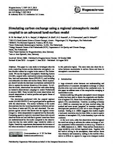
A dry line is a narrow zone where the horizontal gradient of dew point in the PBL is of the order of several degrees per kilometer. It is commonly found over the United States High Plains during the spring months, separating moist air flowing northward from the Gulf of Mexico from dry air flowing eastward from the desert southwest [Schaefer, 1986]. Dry line location and formation are important to local forecasters because deep convection often develops along the dry line [Schaefer, 1986]. In this section we will present an overview of a numerical simulation of a High Plains dry line and associated convection that occurred on April 26, 1991. In previous modeling studies, Ziegler et al. [1995] and Shaw et al. [1997] demonstrated the sensitivity of the dry line to variations in soil moisture in a two-dimensional domain. Horizontal variations in initial soil moisture were found to be necessary for dry line formation. Their conclusions are supported by this study. Furthermore, we will show that convection is impacted when changes in soil moisture alter dry line structure. On the afternoon of April 26, tornadoes formed from supercell thunderstorms that developed along the dry line [U.S. Department of Commerce (USDOC), 1991]. The dry line was oriented north-south in central Kansas and north Oklahoma. Surface observations at 0000 UT, April 27, 1991 (Figure 1), indicated a contrast of 20⬚C in dew point associated with the dry line. At 0031 UT, a visible image from the GOES-7 satellite (Figure 2) showed multiple overshooting tops from the dominant storms, which were aligned with the dry line. The simulations were integrated from 1200 UT, April 26, to 0000 UT, April 27, using four grids with horizontal spacings of 75, 25, 5, and 1.6 km. Details of the setup are shown in Table 1 and are further discussed by Grasso [1999]. Soil moisture was initialized on the two coarsest grids using the API technique and interpolated onto the finest two grids from their respective parent grids. Five simulations were conducted in which only initial soil moisture was varied. The control simulation used the unaltered API soil moisture initialization (Figure 3). In the next three simulations, the initial soil moisture values were altered by multiplying the original values by 0.75, 0.50, and 0.25, respectively. In the final simulation, a horizontally homogeneous soil moisture value was used, roughly corresponding to the grid average of the control values. Results from the control simulation (Figure 4a) show that at 0000 UT on April 27, 1991, convergent winds were coincident with the dry line in north central Oklahoma and south central Kansas. The relatively high dew points west of the dry line over the Kansas-Oklahoma border developed from large latent heat fluxes from the wet soil below. The moistening of the air in that region extended upward a few hundred meters from the surface. As the soil moisture was reduced, the general trend was a weakening of the dry line’s moisture gradient over Oklahoma. The trend, however, was different over Kansas. The simulation with 50% of the full soil moisture had a horizontal gradient of dew point (Figure 4c) similar to the control simulation (Figure 4a), with more convergent winds. As these figures show, a reduction of soil moisture by a factor of 2 resulted in an intensification of the dry line over southwestern Kansas. How-
14,966
BERNARDET ET AL.: SIMULATING CONVECTIVE EVENTS
Figure 1. Surface map at 0000 UT, April 27, 1991. Winds are in m s⫺1 and temperature and dew points are in ⬚C. ever, when the soil moisture was reduced to 25% of the control values, the dew point gradient and the convergence weakened. The location and extension of simulated convection along the dry line exhibited sensitivity to the initial values of soil moisture. Using the midtropospheric vertical velocities on Grid 3 as a proxy for convection, we noted that as the values of soil moisture were altered from 100 to 50%, the coverage of
Figure 2. Goes-7 visible satellite image at 0031 UT, April 27, 1991.
Figure 3. API initialization of volumetric top soil moisture content (m3 m⫺3) on Grid 2, at 1200 UT, April 26, 1991.
BERNARDET ET AL.: SIMULATING CONVECTIVE EVENTS
14,967
Figure 4. Simulated dew point temperature (⬚C) and winds at the lowest model level on Grid 3, at 0000 UT, April 27, 1991, for (a) original API-derived soil moisture initialization; (b) soil moisture initialized at 75% of original value; (c) same as Figure 4b except 50%; (d) same as Figure 4b except 25%; (e) horizontally homogeneous initial soil moisture. Areas with vertical motion in excess of 5.0 m s⫺1 at ⫽ 4832 m are shaded.
convection over Oklahoma decreased, while over Kansas it increased (Figures 4a, 4c). Little convection developed in the simulation with the soil moisture altered to 25% of the control values. No convection developed in the simulation with horizontally homogeneous soil moisture. Although, on average, the dew points in that simulation were the same as those shown in Figure 4a, their horizontal gradient was approximately half and did not characterize a dry line (Figure 4e). Grid 4 was spawned at 2000 UT in the control run. As the simulation advanced, convection intensified along the dry line, and later the cells moved eastward. Figure 5 shows the line of storms in Grid 4 at 2200 UT, and Figure 6 shows a subdomain of Grid 4 with one of the cells. It has characteristics of a supercell thunderstorm, with an updraft core of 30 m s⫺1 collocated with a vertical vorticity maximum of 1.2 ⫻ 10⫺2 s⫺1. The observed storms also had supercell characteristics, presenting hook echoes and reflectivity extremes of 50 dBZ at the 0.5⬚ radar tilt. These simulations demonstrated the sensitivity of dry line frontogenesis and convective development to soil moisture. An
initialization with constant soil moisture led to a diffuse horizontal gradient in the dew point field and no deep convection. Dry line frontogenesis and deep cumulus convection occurred for the simulations with 100, 75, and 50% of the original API values, although the location of the convective developments were different. It is not possible to conclude which of the variable soil moisture initializations (100, 75, or 50% of the API value) led to better simulation results without a detailed verification analysis. However, it is important to note that convection did not develop without the inclusion of variable soil moisture. In the case in which convection developed, it organized in a north south line along the dry line across the Kansas-Oklahoma border (Figure 5), similar to the observations (Figure 2). It should be stressed that soil moisture was initialized on the two coarsest grids only, and therefore its resolution was limited by the 20 km spacing used on the second grid. It remains to be shown how predictable the individual convective cells are when soil moisture is initialized with resolution consistent with the cloud-resolving grid.
14,968
BERNARDET ET AL.: SIMULATING CONVECTIVE EVENTS
Figure 4. (continued)
3.2.
June 30, 1993, High-Precipitation Supercell
The month of July 1993 was characterized by widespread flooding over the American Midwest. Heavy rain, originating from convective events, fell daily from June 29 to July 11. This section presents the simulation of a tornadic supercell thunderstorm that formed on June 30 in northeastern Kansas and later became part of a mesoscale convective complex (MCC), contributing to the period’s rainfall. As is characteristic of the summer months, the convective development had weak upper air support. A large-scale 700hPa trough was present in the western United States at 1200 UT (Figure 7), producing southwesterly flow over Kansas. Significant divergence was observed from 500 to 200 hPa after 1200 UT. The upper level divergence, aided by convergence associated with the southerly low-level jet, sustained this convective event. During the evening of June 29, an MCC developed over
Figure 5. Simulated cloud top temperature (⬚C) on Grid 4 at 2200 UT. The maximum temperature depicted is ⫺20⬚C, and the contour interval is 10⬚C.
Iowa causing heavy rains and strong winds. By 1100 UT, June 30, the system had moved into Illinois. However, new convective cells formed to the west of the system during the early morning hours of June 30, so by sunrise, rain was falling over much of the eastern half of Nebraska and northeastern Kansas. The storm of interest developed between 2100 and 2130 UT, June 30, in northeastern Kansas, at the intersection of a surface stationary front and an outflow boundary generated by the early morning rain over Iowa (Figure 8). Within an hour the storm had become a supercell thunderstorm (Figure 9), and severe weather began to be reported by 2230 UT [USDOC, 1993a]. By 0100 UT on July 1, 1993, this storm had become the southern storm in a squall line that extended from northeast Kansas into central Iowa. Although the system later developed into an MCC, the storm retained its individual supercell characteristics until about 0330 UT on July 1. During the course of its life, the storm moved eastward producing heavy rains (local reports of more than 120 mm in 2 hours in northeastern Kansas), hail as large as 4.5 cm in diameter, and peak winds of 30 m s⫺1). The storm also produced several tornadoes, with six confirmed in northeastern Kansas. To capture the development of the supercell thunderstorm, four grids were used (a detailed description of the evolution of the numerical simulation can be found in the work of Finley [1997]). The coarsest three grids (Table 1) were initialized at the beginning of the simulation (1200 UT on June 30) using data from the NCEP spectral model, rawindsondes, and surface observations. Although the initialization was consistent with the observations at that time, the first attempted simulation failed to produce the rain that occurred in Iowa during the early morning. Without the correct representation of the early convection the outflow boundary, which was observed at 2200 UT (Figure 10a), was not simulated, and the supercell of interest never formed. Stensrud and Fritsch [1994] illustrated the importance of incorporating mesoscale features into the initial conditions of simulations of convection. They presented results from a weakly forced MCC simulation in which outflow boundaries and other mesoscale features not present in the original initialization data were added through the use of “bogus” sound-
Figure 6. Simulated supercell thunderstorm on Grid 4 at 0000 UT, April 27, 1991. Vertical vorticity (⫻10⫺2 s⫺1) (contoured) and vertical velocity (m s⫺1) (shaded– darkest shade is 0 ⬍ w ⱕ 10; medium shade is 10 ⬍ w ⱕ 20; lightest shade is 20 ⬍ w ⱕ 30).
BERNARDET ET AL.: SIMULATING CONVECTIVE EVENTS
Figure 7. The 700-hPa observations and geopotential analysis (m ⫻ 0.1) at 1200 UT, June 30, 1993.
Figure 8. Surface analysis and isotherms (⬚C) at 2200 UT, June 30, 1993. The dashed line represents the outflow boundary that has moved into northern Missouri and northeast Kansas.
14,969
14,970
BERNARDET ET AL.: SIMULATING CONVECTIVE EVENTS
Figure 9. Radar summary at 2235 UT, June 30, 1993. The storm simulated here is developing in northeast Kansas.
ings. Since in the current case the outflow boundary developed after the initialization of the model, a crude form of fourdimensional data assimilation (4-DDA) was used in a subsequent model run to incorporate the outflow boundary. The model solution was nudged toward observations in a limited region of Grid 2 covering northeastern Kansas, southeastern Nebraska, Iowa, and northern Missouri from 1600 to 2000 UT. Hourly surface observations and vertical wind profiler data were used to add forcing terms to the prognostic equations in Grids 2, 3, and 4. In the vertical, nudging was done over a depth of 1 km, the depth of the outflow boundary as indicated by the profiler data. Because thermodynamic data were available only at the surface, their influence was extended through the 1-km nudging region. The nudging weight was constant through the first eight model levels (up to 847 m), dropping off to zero by the eleventh model level (1658 m). Nudging weights and times were chosen to allow the incorporation of the necessary information into the simulation, without creating an imbalance in the solution. Since the outflow developed between 1600 and 1900 UTC, nudging was extended until 2000 UT to attain a more balanced state between the mass and the wind fields. The interior nudging technique was successful in introducing the outflow boundary into the simulation (Figure 10b). The inclusion of thermodynamic information altered the values of temperature and moisture as well. Figure 11 shows the impact nudging had on convective available potential energy (CAPE). Although the temperatures in the nudged case were 3⬚– 4⬚C higher in the storm initiation region at the end of the nudging period (Figure 10), the boundary layer mixing ratios were generally 0.5–1.0 g kg⫺1 lower than in the case without nudging.
The net result was that values of CAPE in the storm initiation region were only ⬃300 J kg⫺1 higher in the nudged case. (Values of convective inhibition were similar in both cases and thus are not shown.) The largest differences in CAPE between the two simulations were located just south of the leading edge of the outflow boundary in Missouri, where CAPE values were up to 1000 J kg⫺1 higher than in the nonnudged simulation due to warmer and moister boundary layer conditions. However, it is unlikely that this region of higher CAPE affected the storm initiation or initial evolution, since the storm only began to cross the Kansas-Missouri border into this area after 0000 UT. To resolve the development of the supercell thunderstorm, Grid 4 was introduced, and the microphysics were activated at 2000 UT. Grid 4 was initially centered over the intersection of the stationary front and the outflow boundary, since boundary layer convergence on Grid 3 exhibited an extrema of ⫺1.0 ⫻ 10⫺3 s⫺1 in that region. At 2130 UT the storm began to develop, and 18 min later it went through a splitting process, from which a cyclonically rotating right moving supercell evolved. The characteristics of the convection (isolated supercell) as well as the forcing mechanism (convergence at the intersection of the front and the outflow boundary were similar to the observed ones. The simulated storm, however, developed ⬃50 km to the east of the observed one. The storm moved eastward along the original outflow boundary, while new convective elements developed westward, along the stationary front. At 2348 UT the rain pattern developed a hook shape and the rain rates approached 120 mm h⫺1, characterizing the cell as a high-precipitation (HP) supercell [Moller et al., 1994]. The evolution of the supercell is shown in Figure 12. Finley [1997] describes the inclusion of two other
BERNARDET ET AL.: SIMULATING CONVECTIVE EVENTS
14,971
nested grids, lowering the grid spacing to 100 m to simulate tornado genesis. In this case, the focusing mechanism for storm development was the surface convergence associated with the intersection between a stationary front and an outflow boundary generated by previous convection. Interior nudging was necessary since the simulation did not develop in the morning convection spontaneously. The nudging method is controversial because as it forces the model solution toward the observations, it causes the simulation to deviate from its own solution. Nudging may also destroy important and realistic small scale struc-
Figure 11. Simulated convective available potential energy (J kg⫺1) at 2000 UT for the simulation (a) without 4-DDA and (b) with 4-DDA.
tures existent in the simulation but not present in the data. From this experience, however, it appears that if nudging is turned off early enough in the simulation, it can be used to introduce the necessary mesoscale features to initiate a storm without further interference with the simulation. 3.3.
Figure 10. Simulated surface temperature (⬚C) and winds for the simulation (a) without 4-DDA at 2145 UT, June 30, 1993, and (b) with 4-DDA at 2148 UT, June 30, 1993, on Grid 3. Areas with water condensate in excess of 1.0 g kg⫺1 at ⫽ 5113 m are shaded. No significant condensate was present at in the simulation without 4-DDA.
July 19, 1993, Mesoscale Convective System
The organization of clouds in MCSs is of interest to forecasters because certain MCS types are associated with particular severe weather characteristics (e.g., bow echoes and strong winds) and because MCSs last longer than individual thunderstorms. MCCs, in particular, can last for several days and cover thousands of kilometers through a regeneration process [Fritsh et al., 1994]. This section describes a simulation of the developing stages of a small MCS that formed in northeastern Colorado on July 19, 1993. The first storms formed over the foothills of the Colorado Rocky Mountains; as the system moved eastward onto the plains, individual convective cells became organized in a MCS. The environmental factors that led to system organization and their importance to the forecast will be discussed. At upper levels, a deep trough was located over the western
14,972
BERNARDET ET AL.: SIMULATING CONVECTIVE EVENTS
Figure 12. Simulated condensate mixing ratio g kg⫺1 at the lowest model level on Grid 4 at (a) 2148 UT on June 30, 1993; (b) 2307 UT on June 30, 1993; (c) 0000 UT on July 1, 1993; (d) 0049 UT on July 1, 1993. Contour interval is 0.5 g kg⫺1. United States at 0000 UT on July 19, 1993. Most of northeastern Colorado was beneath the right entrance region of a 200 hPa jet streak, an area where large-scale upward motion prevails. The 500 hPa flow over northern Colorado was 15 m s⫺1, strong for this time of the year. At 850 hPa a low-level jet (LLJ) extended from southern Texas into Wyoming, transporting moist air into the High Plains. Warm advection was occurring from northeastern Colorado into eastern Wyoming and western Nebraska. A quasi-stationary ill-defined east-west surface front extended through northern Colorado and Kansas (Figure 13). A southeasterly gradient flow combined with diurnal upslope brought deep moisture westward from the rain-soaked plains. Surface dew points near the foothills were very high as a result, with values at or above 15⬚C. The first convective cells appeared on radar soon after 1800 UT (local noon). The strongest cells formed over the high terrain west of Denver, Colorado. To simulate this system, four
grids were used. Grids 1–3 were initialized at 1200 UT, while Grid 4 was initialized along with the full microphysics at 1800 UT. A detailed description of this simulation can be found in the work of Nachamkin [1998] and Nachamkin and Cotton [1999a, b]. Simulated convection developed over the high terrain at 1900 UT. Several cells were positioned along the Continental Divide, with the cells with the largest updraft speeds located in the south, just west of Denver. To obtain convection with reasonable characteristics along the Continental Divide, the values of initial soil moisture had to be altered from the ones produced by the API method described in section 2. The original soil moisture analysis over the mountains was too dry due to the very small number of rain gages, the snow undercatchment by the gages, and the underrepresentation of liquid water from snow older than the 3-month period considered by the API analysis. The API dry bias resulted in an unrealistically strong mountain-plains solenoid circulation and associated
BERNARDET ET AL.: SIMULATING CONVECTIVE EVENTS
14,973
Figure 13. Surface map at 1800 UT on July 19, 1993. Winds are in m s⫺1 and temperature and dew points are in ⬚C. Mean sea level pressure is contoured every 4 hPa.
convection. To alleviate this problem, the original soil moisture in the region above 1700 m was linearly increased with height from 0.06 to 0.18 m3 m⫺3 at 2700 m. The organization of convection in the simulation was similar to the radar observations. The initial cells located over the high terrain moved eastward. While the northern storms dissipated, the updraft speed increased to 25 m s⫺1 within the southern cell. Several new convective storms formed in the vicinity of the original southern cell, and by 2100 UT, two dominant cells emerged (Figure 14), giving origin to the MCS. The simulated placement and orientation of the main convection agreed well with the radar observations (Figure 15). Simulated convection along the northern Front Range was more persistent than observed. The radar detected weak echoes in that location between 1800 and 1900 UT, but they rapidly dissipated. Simulated convection in the northern Front Range remained weak (updrafts not exceeding 5 m s⫺1 and moved northward out of Grid 4 by 2100 UT. At 2130 UT the simulated 5-min rain rate associated with the MCS already exceeded 130 mm h⫺1. By 2200 UT the storms intercepted a convergence zone southeast of Denver, and the cells became aligned in the north-south direction. At this time, the cloud tops reached ⫺60⬚C, a cold pool developed, and the simulated convection became less dependent on preexisting convergence zones for convective lift. Figure 16 presents the evolution of the MCS as seen by radar and can be compared with the model output in Figure 17. Note that the figures are not at the exact same time or domain and should be used solely for an overview. By 2230 UT (Figure 16b) the radar
showed that the system had developed a bow echo shape, which also developed in the simulation. Hail, strong winds, and heavy rain accompanied the system as it propagated eastward [USDOC, 1993b]. Convective propagation was best simulated early in the run. Both the modeled and the observed storms attained a bow echo structure for less than 1 hour as they passed through the convergence zone east of Denver around 2230 UT. As the system propagated eastward, the model solution slowly deviated from the observations. By the time the simulated storm reached the Colorado-Kansas border, it was ⬃1 hour behind the observed one. The general placement and linear structure, however, were retained. Several regional circulations focused the initial convective development. The mountain-plains solenoid, generated by differential daytime heating between the mountains and the plains, provided the upslope necessary for the first storms to develop. As the storms moved east toward Denver, surface convergence associated with the Denver Convergence and Vorticity Zone (DCVZ) [Szoke et al., 1984] enhanced the updraft speeds. The cooler temperatures to the north of the stationary front were instrumental in suppressing initial convection that moved eastward north of Denver. The storms also suffered the detrimental effects of the subsident branch of the mountain-plains solenoid [Tripoli and Cotton, 1989a, b] as they moved east. However, the storms that propagated along the Palmer Divide were subject to less of this effect, since the elevated terrain weakened the solenoid locally [Nachamkin and Cotton, 1998]. The intensification of the MCS was also determined by the upward branch of the Platte Valley-Palmer
14,974
BERNARDET ET AL.: SIMULATING CONVECTIVE EVENTS
Figure 14. Topography and simulated surface winds (m s⫺1) on Grid 3 at 2100 UT on July 19, 1993. Areas with water condensate in excess of 1.0 g kg⫺1 at ⫽ 5000 m are shaded. Divide (PVPD) solenoid, a north-south solenoidal circulation that develops on the northern slope of the Palmer Divide due to differential heating [Toth and Richardson, 1985]. Between 2300 and 0000 UT both the simulated and the observed MCSs entered their mature phase, as indicated by a rapid growth in the cloud shield and a tripling in the simulated and observed volumetric system-total rain rates. The simulated fields revealed that this growth occurred when the MCS interacted with an intense but localized southerly LLJ (Figure 18). The jet formed over southeast Colorado at 2100 UT, and the maximum winds were located at the top of the mixed boundary layer, or at about 1500 m above ground level (agl). The entire feature was only 200 km wide, with winds of up to 20 m s⫺1. This jet also developed in a simulation with microphysical processes turned off (which prevented deep convection from forming in the simulation), indicating that the jet was not caused by the MCS. Instead, the jet was associated with a region of thermally induced low pressure located in northeast Colorado, where diurnal heating resulted in a warm and wellmixed PBL. East of Limon, Colorado, the temperatures were lower and the pressure was higher because of the relatively large soil moisture content. Given the eastward pressure gradient, geostrophic adjustment determined the southerly flow. In summary, convection was focused on this day by the synoptic scale front and by the circulations associated with differential heating in complex topography. The mountainplains and PVPD solenoids, coupled with the stationary front and the thermally induced LLJ were instrumental in determining the regions favorable for convection, and therefore the location of the MCS. The model was able to simulate this system well within its finer grids because the terrain, the preexisting synoptic front and the surface, and PBL processes were well resolved. 3.4.
May 12, 1985, Derecho
Derechos are convectively induced windstorms with typical lifetimes of 8 hours or more [Bentley and Mote, 1998]. They are
associated with severe storms and frequently occur at night on the cold side of a thermal boundary and over a stable boundary layer. Derecho-producing storms can many times be characterized as elevated thunderstorms, since the unstable air responsible for storm maintenance is not surface based but comes from an elevated source, such as the LLJ, which develops on a scale quite larger than the individual thunderstorms or MCS associated with the derecho. Elevated thunderstorms are difficult to forecast and have been pointed out by McNulty [1995] as one of the most challenging forecast problems for the National Weather Service. One source of forecasting difficulty is that models with large grid spacings use cumulus parameterizations which are usually not triggered when the lower levels are highly stable. High-resolution models may be necessary to capture derecho events and to resolve the details of cloud organization and wind gust intensity. The case described in this section is the longest simulation presented in this study. Severe weather associated with this event was reported between 0600 and 1200 UT on May 13, 1985, but the convective system itself began developing late in the afternoon of May 12, 1985, in southeastern Colorado. The model was initialized at 1200 UT on May 12, 1985, and integrated for 24 hours. Most of the analysis will focus on the first 17 hours, during which the simulated derecho reached maximum intensity. The synoptic environment at 0000 UT May 13, 1985, included a stationary surface front that extended eastward from the Texas Panhandle through Oklahoma (Figure 19). A surface low was located on the border of the Texas Panhandle and New Mexico and a weak high was over Nebraska. At 850 hPa the lowest geopotential heights were located over central New Mexico, resulting in southeast winds over the MCS genesis
Figure 15. Surface mesonet and low-level reflectivity analysis at 2058 UT, July 19, 1993. Winds are in m s⫺1 and one full barb is equal to 5 m s⫺1. Reflectivity from the CSU-CHILL radar at 2 km agl is contoured every 7.5-dBZ intervals, starting at 15 dBZ, with shading increments at 15, 30, and 45 dBZ. Distance north and east is plotted in kilometers on the left and bottom axes and in latitude and longitude on the right and top.
BERNARDET ET AL.: SIMULATING CONVECTIVE EVENTS
14,975
Figure 16. Same as Figure 15 except for (a) 2155 UT, July 19, 1993; (b) 2230 UT, July 19, 1993; (c) 2330 UT, July 19, 1993; and (d) 0055 UT, July 20, 1993.
region. The 700 and 500 hPa trough axis extended over Colorado and Texas and the mean upper level winds over the region were southwesterly (Figure 20). The Limon, CO, radar showed that at 0035 UT May 13, 1985, only light precipitation existed over southeastern Colorado. By 0130 UT, two strong cells had developed in Las Animas county, and at 0330 UT, several cells were present in that region, aligned in an approximately east-west line (Figure 21). A region of stratiform precipitation was located to the north of the convective line, while the convective cells were moving from 256⬚ with an average speed of 17 m s⫺1. Since the focus of this simulation was the storms that caused the severe winds, four grids were used (Table 1), with the finest horizontal spacing of 2 km. As the storms did not begin until late afternoon, the simulation was initialized at 1200 UT on May 12 with only the three coarsest grids. At 2000 UT the fourth grid was introduced and the full microphysics parameterization was initiated. This time coincided with the development, in the simulation, of a north-south convergence line parallel to the foothills of the Colorado Rockies. The conver-
gence developed as a result of diurnal heating and propagated eastward over the next hour. At 2100 UT the first simulated storm developed along this convergence line, and by 2300 UT, moist convection became deep and organized. The convection organized in a line parallel to the topography. At 0000 UT, two cells merged and produced a strong cold pool, with a surface temperature 4⬚C lower than the prestorm environment. New convection developed on the northeasterly outflow on the rear of the storm, causing the line to reorient in the east-west direction, as it continued to move eastward (Figure 22). The results of a trajectory and equivalent potential temperature ( e ) analysis (discussed by Bernardet and Cotton [1998]) indicate that at this time, the source of air for convection was located near the surface, consistent with the observations of a daytime well-mixed PBL. The distribution of the convective cells was similar to the radar-observed pattern (Figure 21). The simulated system consisted of a line of three cells oriented in the east-west direction, with a small amount of condensate between the cells. It should be noted that deep tropospheric convection developed in the model 3 hours earlier than ob-
14,976
BERNARDET ET AL.: SIMULATING CONVECTIVE EVENTS
Figure 17. Simulated total condensate and wind vectors on Grid 3 at the lowest model level at 2200 UT, July 19, 1993; (b) 2330 UT, July 19, 1993; (c) 0030 UT, July 20, 1993; and (d) 0300 UT, July 20, 1993. The locations of the CHILL (CH) and mile high (MH) radars as well as a few NWS reporting stations are plotted. The position of Grid 4 is indicated by the rectangle. Total condensate greater than 0.1 g kg⫺1 is shaded, and values above 0.5 g kg⫺1 are contoured at 0.5 g kg⫺1 increments. Vectors are plotted in m s⫺1 according to the scale at the bottom of each panel. served and that the simulated line was oriented east-west, while the observed line was in a northeast-southwest direction. During the evening, the observed surface low and front remained almost stationary, while the high moved eastward to Minnesota. This contributed to easterly winds over Kansas, which fed into the convective system. By 1200 UT on May 13, the 850 hPa low had deepened and moved to the Oklahoma panhandle. The southerly winds over Kansas at 1 km agl increased from 1 to 12 m s⫺1 between 0000 and 1200 UT on May 13, indicating the development of the LLJ, which was reproduced in the simulation (Figure 23). At 700 hPa, a closed low developed over eastern Colorado, and the upper level trough axis was over central Colorado and New Mexico. Consequently, southerly winds were observed through most of the troposphere over Kansas. The observed thermodynamic pro-
file over western Kansas at 1200 UT was characterized by a stable layer from the surface (920 hPa) to 800 hPa. This contrasted with the profile observed in the same location during the previous afternoon, which displayed a 200 hPa deep wellmixed surface-based boundary layer, characteristic of the initial stages of derecho development. Radar observations showed that by 0535 UT the storms had entered Kansas, where they continued to move northeastward until the system weakened before sunrise at the Kansas-Nebraska border. Although only one tornado was confirmed, this system left behind a narrow swath of damage caused by winds stronger than 26 m s⫺1 extending for 400 km from western to northern Kansas [USDOC, 1985], characterizing this event as a derecho. In the model, a stable boundary layer developed after sunset, which enhanced the stability on the northern side of the front,
BERNARDET ET AL.: SIMULATING CONVECTIVE EVENTS
Figure 18. Simulated meridional wind component (m s⫺1) at z ⫽ 3000 m on Grid 2 at 0000 UT, July 19, 1993. Areas of condensate in excess of 0.1 g kg⫺1 at this level are shaded. where the MCS was located. Parcels of air originating near the surface became stable with respect to vertical displacements and, for the most part, did not reach the level of free convection. However, at this time the LLJ developed over Oklahoma and advanced northward above the front (Figure 24). The LLJ
14,977
had two origins. One was the eastward movement of the midlevel trough, which caused the winds to turn from southwest to southerly over the MCS region. The other was thermal factors associated with the east-west gradient of temperature across the High Plains [McNider and Pielke, 1981]. Since the low-level winds over Kansas had an easterly component, the high- e air brought by the LLJ was transported westward to the region of MCS development in eastern Colorado (Figure 25). This unstable air was then ingested by the storms, as shown in Figure 26. The nocturnal phase of the simulated storms was characterized by strong rotation, as the storms assumed characteristics of HP supercells. The rain rates were very high (up to 114 mm h⫺1) and vertical vorticity reached 10⫺2 s⫺1 at a height of 3 km. The rotation and its associated pressure deficit caused the upward displacement of parcels out of the stable boundary layer. As those parcels were lifted, their negative buoyancy was enhanced, ultimately leading to the development of the downdraft and surface winds, as discussed by Bernardet and Cotton [1998]. The simulated storms followed a track similar to the radar-observed ones and produced winds of over 20 m s⫺1 for eight and a half hours (Figure 27). The characterization of the MCS in this simulation was dependent on the synoptic scale flow, the PBL development, and the topography representation. In the initial stages of development the MCS was triggered by a convergence line associated with the differential diurnal heating between the foothills of the Rocky Mountains and the plains to the east. A daytime well-mixed PBL was present and supplied unstable air to the system. During the night a stable PBL developed on the cold side of the stationary front and was instrumental to the
Figure 19. Surface map at 0000 UT, May 13, 1985. Winds are in m s⫺1 and temperature and dew points are in ⬚C.
14,978
BERNARDET ET AL.: SIMULATING CONVECTIVE EVENTS
Figure 20. The 700-hPa analysis at 0000 UT, May 13, 1985. development of the damaging surface winds. Without access to surface-based unstable air the system relied on the LLJ for its maintenance. The development of the LLJ was tied to local heating heterogeneities associated with the slope of the plains toward the west. However, it also had a synoptic scale component, associated with the eastward movement of a midlevel trough. Therefore the multiscale aspect of this simulation was very important. The development of the LLJ in Grids 2 and 3 was communicated via lateral boundaries to Grid 4, where it interacted with the convective system.
4.
Discussion
In the previous section, mesoscale simulations of convective events were analyzed with the goal of giving insight into the necessary characteristics of numerical models or model setup that lead to the development of convective systems. As stated in the introduction, this analysis was exploratory and did not use an objective methodology (such as extensive sensitivity studies) to identify the factors that must necessarily be included in a model. Instead, model output was inspected subjectively for similarity to the observations. Storm location and timing, as well as convective organization (isolated versus organized in MCSs) were some of the aspects used to determine the success of the simulations. In the cases described here, satisfactory simulations were achieved even though alterations in the input data were necessary in two cases. As expected, agreement between observations and model output is not perfect. In some cases the simulated storm is a few hours off, or a few tens of kilometers away from the observed one. However, the sole fact that a storm with the correct organization was simulated in the general vicinity and timing of the observations can be considered a success. A model that provides guidance as
to the onset of convection, its general location, time, and organization (e.g., severe or not) is a useful forecasting tool, even if the predicted storm’s timing and location are not exact. Four significantly different systems were studied: two cases of supercell thunderstorms and two of MCSs. The location and season of development for all systems was similar: all four formed on the Plains, east of the Rocky Mountains. None of the systems was triggered by synoptic scale boundaries, as occurs with prefrontal squall lines. Instead, the systems were initiated by topography, or soil moisture gradients or other mesoscale forcing features. The results showed that a fine grid with spacing of the order of 2 km was sufficient to capture convection explicitly. In some of the cases, convection actually developed in the grid with 5 km spacing. In the July 19, 1993 case, convection was focused by the presence of a 200 km wide thermally driven LLJ, with an axis of 20 m s⫺1 winds only 50 km wide. The use of highresolution grids was necessary in this case not only to resolve the convection but also to resolve the jet strength, timing, and location. The importance of such a small-scale environmental feature was revealed by the rapid growth of the MCS after it interacted with the jet, resulting in the tripling of the volumetric rain rate. In this same case the system developed along a convergence zone associated with the DCVZ, a small-scale environmental feature that can only be resolved in a regional scale model (10 km or less in grid spacing). The genesis of two of the convective events discussed was related to topographical features, pointing to the importance of the accurate representation of topography in the models. In the May 12, 1985, case, the system started as a north-south line oriented parallel to the Rocky Mountains, forced by a convergence zone associated with the diurnal thermal structures that
BERNARDET ET AL.: SIMULATING CONVECTIVE EVENTS
were associated with the terrain. After the system formed, it relied on its own cold pool dynamics to reorientate to the east-west direction. A similar situation happened in the July 19, 1993, case. The first cells formed on the high terrain east of the Colorado Rocky Mountains. As the convective elements moved eastward, most of them were suppressed by the subsidence associated with the descending branch of the mountainplains solenoid. However, the cells that moved eastward over the Palmer Divide remained active because the subsidence was weakened locally by the elevated terrain and because there was upward motion associated with the ascending branch of the PVPD solenoid, also a terrain-driven circulation. The sensitivity of the systems to the topography is directly associated with the thermal and wind distribution caused by the topography. The correct representation of the mass and wind fields is the ultimate product of all the numerics and physics of the model working in concert, and directly involves the radiation, soil, vegetation, surface layer, turbulence, and cloud microphysics parameterizations. A dependence on topography features was absent in the two supercell cases. The June 30, 1993, supercell developed in northeastern Kansas, a region far from significant gradients of topography. The April 26, 1991, supercell developed along a dry line. Topography may have contributed to dry line formation, but our sensitivity studies demonstrated that in this case, the dry line did not undergo frontogenesis, and its associated convection did not form unless horizontal gradients of soil
Figure 21. Reflectivity analysis for 0330 UT, May 13, 1985. The PPI from the Limon radar at 0.5⬚ is contoured every 7.5-dBZ intervals, starting at 15 dBZ, with shading increments at 15, 30, and 45 dBZ. The rectangle in bold lines represents the location of the model Grid 4 at this time.
14,979
Figure 22. Simulated water condensate (g kg⫺1) at the lowest model level on Grid 4 at 0330 UT, May 13, 1985.
Figure 23. Vertical profile of (a) observed and (b) simulated meridional winds at latitude ⫽ 38⬚N and longitude ⫽ 98⬚W.
14,980
BERNARDET ET AL.: SIMULATING CONVECTIVE EVENTS
Figure 24. Simulated vertical cross section of equivalent potential temperature (K) through longitude ⫽ 97.5 W on Grid 2 at 0500 UT, May 13, 1985. Regions with meridional wind speed larger than 12 m s⫺1 are shaded.
moisture were present in the model initialization. Future studies will focus on the frontogenetic forcing of the low-level water vapor field associated with the April 26, 1991, dry line. Also planned is an examination of the baroclinicity at the dryline and of the distribution of sensible and latent heat fluxes to understand the exact role played by soil moisture in dry line intensification. Soil moisture was also very important in the July 19, 1993, case. It led to the development of a thermal
gradient, which forced the winds into a LLJ. The importance of this jet to the growth of an MCS was described in section 3.3. In the course of this analysis, factors were revealed that were not crucial to particular simulations. The May 12, 1985, simulation was initialized with a horizontally homogeneous distribution of soil moisture and was still able to reproduce the system. However, since soil moisture initialization was crucial to the April 26, 1991 and July 19, 1993, cases and since it is not possible to know a priori which cases will depend on it, it has to be included in models designed to simulate or forecast convective events. In the May 12, 1985, derecho case, atmospheric features played a more important role than soil moisture gradients, although the actual soil moisture magnitude was important. The synoptic conditions changed significantly from day to night, as a midlevel synoptic scale trough moved into the area. This trough and the thermal effects associated with the westward slope of the plains were responsible for the development of a nocturnal LLJ in the area. The jet sustained the system through the night, since the PBL was stable and nonconducive to convection. Therefore the accurate representation of synoptic scale features is of fundamental importance to mesoscale simulations. Finally, we would like to point out the need for 4-DDA (interior nudging) in the June 30, 1993, case. Although the fine grids used in all other cases were sufficient to resolve the triggering mechanisms for the storms, this was not the case with the morning convection on June 30, 1993. The reason is that this early convection began before 1200 UT and was already producing rain when the model was initialized. At time zero the model is initialized with zonal and meridional wind speeds, pressures, temperature, and water vapor but with zero
Figure 25. Simulated meridional winds (m s⫺1) and wind barbs at ⫽ 1043 m at 0500 UT, May 13, 1985. Regions with condensate mixing ratio in excess of 0.5 g kg⫺1 at ⫽ 4831 m are shaded to denote storm location.
BERNARDET ET AL.: SIMULATING CONVECTIVE EVENTS
vertical velocity or supersaturation, i.e., without clouds. An adjustment period of a few hours is expected until clouds develop in the simulation. If the system of interest occurs during that spin-up time, or if it occurs later but depends on features that develop during the adjustment time, the simulation may not be successful. It follows from the above that some mechanism of dynamic initialization of the model with clouds (“hot start”) and/or 4-DDA is necessary for the success of the early and later hours of forecast in some cases. This has been an area of debate within the numerical weather prediction community [Zhao et al., 1998], but measurable results are yet to emerge. The use of nudging for real-time forecasting has the drawback of causing a delay, since the model can only be initialized after the observations for the subsequent hours have been taken and communicated to the weather office. The lead time for the forecast product is therefore shorter. However, if nudging, or another form of 4-DDA, leads to an improved forecasting product, there is reason to use it. Note that a delay also occurs with the adjoint method of model initialization, which involves integrating the model forward, the adjoint backward, and the model forward again. The results presented are not conclusive but only represent a first step toward determining the characteristics of models designed to explicitly represent convection. One important aspect that was not examined in this study is the sensitivity of the modeled storms to the initial atmospheric conditions, which may be particularly strong in weakly forced cases of convection. Several authors have examined this problem and some [e.g., Sindic-Rancic and Kalnay, 1998] have suggested the use of an ensemble composed of different model initializations to obtain a range of possible solutions, which would be used to compute forecast probabilities. The findings of this study remain valid whether probabilistic or deterministic forecasts are performed, since the best possible high-resolution model should be used in either case. Another aspect that should be further investigated is the sensitivity of the results to physiography resolution. In the June
14,981
Figure 27. Time series of simulated winds at the lowest model level on Grid 4 from 2200 UT, May 12, 1985, to 1200 UT, May 13, 1985. The solid circles represent the maximum speed in the horizontal domain and the open circles, the maximum speed found in a convective outflow. After 0300 UT they coincide. 30, 1993, case, the finest resolution of terrain was on Grid 3, with 8-km spacing. In the July 19, 1993 and the May 12, 1985, cases, terrain was defined on Grid 2 with 20-km and 40-km horizontal spacing, respectively. Topography was then interpolated to the finest grids. Soil moisture was initialized only in the coarsest grid of each simulation, except for the April 26, 1991, case, in which it was also initialized in Grid 2. It seems likely that the precision in temporal and spatial prediction of the storms was limited by the resolution in physiography.
5.
Conclusions
Simulations of four convective events were analyzed to give insight into model characteristics which are important to forecasting convective events. These characteristics vary from case to case and include high-resolution grids, adequate lateral boundary conditions that communicate quickly and effectively changes in the synoptic conditions to the finer grids, adequate initial soil moisture distribution, good representation of topographical features, and dynamic initialization of clouds or of mesoscale features that favor cloud development during the early stages of the simulation. Acknowledgments. Support for this research was provided by the National Science Foundation under grants ATM-9900929, ATM9420045, ATM-9118963, ATM-8919080, and ATM-9306754 and by CAPES (Coordenac¸˜o a de Aperfeic¸oamento de Pessoal de Nı´vel Superior), Brazil. Thank you to John Snook, Adrian Marroquin, Nita Fullerton, and two anonymous reviewers for their suggestions, which much improved this manuscript.
References Figure 26. Simulated vertical cross section of equivalent potential temperature (K) through latitude ⫽ 38.0⬚N on Grid 4 at 0500 UT, May 13, 1985. Areas of water condensate in excess of 2 g kg⫺1 are shaded.
Avissar, R., and R. A. Pielke, A parameterization of heterogeneous land surface for atmospheric numerical models and its impact on regional meteorology, Mon. Weather Rev., 114, 330 –343, 1989. Benjamin, S. G., K. A. Brewster, R. Brummer, B. F. Jewett, T. W. Schlatter, T. L. Smith, and P. A. Stamus, An isentropic three-hourly assimilation system using ACARS aircraft observations, Mon. Weather Rev., 119, 888 –906, 1991.
14,982
BERNARDET ET AL.: SIMULATING CONVECTIVE EVENTS
Bentley, M. L., and T. L. Mote, A climatology od derecho-producing mesoscale convective systems in the central and eastern United States, 1986 –95, part I, Temporal and spacial distribution, Bull. Am. Meteorol. Soc., 79, 2527–2440, 1998. Bernardet, L. R., and W. R. Cotton, Multiscale evolution of a derechoproducing mesoscale convective system, Mon. Weather Rev., 126, 2991–3015, 1998. Black, T. L., The new NMC mesoscale Eta model: Description and forecast examples, Weather Forecasting, 9, 265–278, 1994. Cotton, W. R., G. Thompson, and P. W. Mielke, Real-time mesoscale prediction on workstations, Bull. Am. Meteorol. Soc., 75, 349 –362, 1994. Davies, H. C., Limitations of some common lateral boundary schemes used in regional NWP models, Mon. Weather Rev., 111, 1002–1012, 1983. Droegemeier, K. D., SAMEX December 1997 Newsletter, 1997. (Available as http://www.caps.ou.edu/CAPS/samex/SAMEX.nwsltr.html) Finley, C. A., Numerical simulation of intense multi-scale vortices generated by supercell thunderstorms, Atmos. Sci. Pap. 640, 297 pp., 1997. (Available from Dep. of Atmos. Sci., Colo. State Univ., Fort Collins) Fritsch, J. M., R. J. Kane, and C. R. Chelius, The contribution of mesoscale convective systems to the warm season precipitation in the United States, J. Clim. Appl. Meteorol., 25, 1333–1345, 1986. Fritsch, J. M., J. D. Murphy, and J. S. Kain, Warm-core vortex amplification over land, J. Atmos. Sci., 51, 1780 –1807, 1994. Gal-Chen, T., and R. C. J. Sommerville, On the use of a coordinate transformation for the solution of the Navier-Stokes equations, J. Comput. Phys., 17, 209 –228, 1975. Grasso, L. D., A numerical simulation of dryline sensitivity to soil moisture, Mon. Weather Rev., in press, 1999. Hill, G. E., Factors controlling the size and spacing of cumulus clouds as revealed by numerical experiments, J. Atmos. Sci., 31, 646 – 673, 1974. Lilly, D. K., On the numerical simulation of buoyant convection, Tellus, 2, 148 –172, 1962. Louis, J. F., A parametric model of vertical eddy fluxes in the atmosphere, Boundary Layer Meteorol., 17, 187–202, 1979. Louis, J. F., M. Tiedke, and J.-F. Geleyn, A short history of the PBL parameterization at the ECMWF, in Workshop on Planetary Boundary Layer Parameterization, pp. 59 – 80, Eur. Cent. for MediumRange Weather Forecasts, Reading, England, 1981. Loveland, T. R., J. W. Merchant, D. O. Ohlen, and J. F. Brown, Development of a landcover characteristics database for the conterminous U.S., Photo. Eng. Remote Sens., 57, 1453–1463, 1991. Mahrer, Y., and R. A. Pielke, A numerical study of the airflow over irregular terrain, Beitr. Phys. Atmos., 50, 98 –113, 1977. Mass, C. F., and Y.-H. Kuo, Regional real-time numerical weather prediction: Current status and future potential, Bull. Am. Meteorol. Soc., 79, 253–263, 1998. McNider, R. T., and R. A. Pielke, Diurnal boundary layer development over sloping terrain, J. Atmos. Sci., 38, 2198 –2212, 1981. McNulty, R. P., Severe and convective weather: A central region forecasting challenge, Weather Forecasting, 10, 187–202, 1995. Moller, A. R., C. A. Doswell, M. P. Foster, and G. R. Woodall, The operational recognition of supercell thunderstorm environments and storm structures, Weather Forecasting, 9, 327–347, 1994. Nachamkin, J. E., Observational and numerical analysis of the genesis of a mesoscale convective system, Atmos. Sci. Pap. 643, 219 pp., 1998. (Available from Dep. of Atmos. Sci., Colo. State Univ., Fort Collins) Nachamkin, J. E., and W. R. Cotton, Interacting solenoidal circulations and their role in convective orogenesis, in Proceedings of the 8th Conference on Mountain Meteorology, pp. 297–301, Am. Meteorol. Soc., Boston, Mass., 1998. Nachamkin, J. E., and W. R. Cotton, Interactions between a developing mesoscale convective system and its environment, part I, Observational analysis, Mon. Weather Rev., in press, 1999a. Nachamkin, J. E., and W. R. Cotton, Interactions between a developing mesoscale convective system and its environment, part II, Numerical simulation, Mon. Weather Rev., in press, 1999b. Pielke, R. A., et al., A comprehensive meteorological modeling system—RAMS, Meteorol. Atmos. Phys., 49, 69 –91, 1992. Schaefer, J. T., The dryline, in Mesoscale Meteorology and Forecasting, edited by P. S. Ray, pp. 549 –570, Am. Meteorol. Soc., Boston, Mass., 1986. Shaw, B. L., R. A. Pielke, and C. L. Ziegler, A three-dimensional numerical simulation of a Great Plains dryline, Mon. Weather Rev., 125, 1489 –1506, 1997.
Sindic-Rancic, G., and E. Kalnay, Storm scale ensemble experiments with the ARPS model: Preliminary results, in Proceedings of the 12th Conference on Numerical Weather Forecasting, pp. 279 –280, Am. Meteorol. Soc., Boston, Mass., 1998. Smagorinsky, J., General circulation experiments with the primitive equations, part I, The basic experiment, Mon. Weather Rev., 91, 99 –164, 1963. Snook, J. S., P. A. Stamus, J. P. Edwards, Z. Christidis, and J. A. McGinley, Local-domain analysis and forecast model support for the 1996 Centennial Olympic Games, Weather Forecasting, 13, 138 –150, 1998. Staudenmaier, M., Jr., and J. Mittelstadt, Results of the western region evaluation of the Eta-10 model, in Proceedings of the 12th Conference on Numerical Weather Prediction, pp. 131–134, Am. Meteorol. Soc., Boston, Mass., 1998. Stensrud, D. J., and J. M. Fritsch, Mesoscale convective systems in weakly forced large-scale environments, part II, Generation of a mesoscale initial condition, Mon. Weather Rev., 122, 2068 –2083, 1994. Szoke, E. J., M. L. Weisman, J. M. Brown, F. Caracena, and T. W. Schlatter, A sub-synoptic analysis of the Denver tornado of 3 June, 1981, Mon. Weather Rev., 112, 790 – 808, 1984. Toth, J. J., and R. H. Richarson, Summer surface flow characteristics over northeastern Colorado, Mon. Weather Rev., 113, 1458 –1469, 1985. Tremback, C. J., and R. Kessler, A surface temperature and moisture parameterization for use in mesoscale numerical models, in Proceedings of the 7th Conference on Numerical Weather Prediction, pp. 355–358, Am. Meteorol. Soc., Boston, Mass., 1985. Tripoli, G., and W. R. Cotton, A numerical study of an observed orogenic mesoscale convective system, part 1, Simulated genesis and comparison with observations, Mon. Weather Rev., 117, 273–304, 1989a. Tripoli, G., and W. R. Cotton, A numerical study of an observed orogenic mesoscale convective system, part 2, Analysis of governing dynamics, Mon. Weather Rev., 117, 305–328, 1989b. U.S. Department of Commerce (USDOC), Storm Data, 27(5), 1– 66, 1985. U.S. Department of Commerce (USDOC), Storm Data, 33(4), 1–239, 1991. U.S. Department of Commerce (USDOC), Storm Data, 35(6), 1–289, 1993a. U.S. Department of Commerce (USDOC), Storm Data, 35(7), 1–300, 1993b. Walko, R. L., W. R. Cotton, M. P. Meyers, and J. Y. Harrington, New RAMS cloud microphysics parameterization, part I, The singlemoment scheme, Atmos. Res., 38, 29 – 62, 1995. Weisman, M. L., W. C. Skamarock, and J. B. Klemp, The resolution dependence of explicitly modeled convective systems, Mon. Weather Rev., 125, 527–548, 1997. Wetzel, P. J., and J. T. Chang, Evapotranspiration from non-uniform surfaces, A first approach for short-term numerical weather prediction, Mon. Weather Rev., 116, 600 – 621, 1988. Zhang, D.-L., E.-Y. Hsie, and M. W. Moncrieff, A comparison of explicit and implicit predictions of convective and stratiform precipitating weather systems with a meso--scale numerical model, Q. J. R. Meteorol. Soc., 114, 31– 60, 1988. Zhao, Q., T. L. Black, G. J. DiMego, R. Aune, Y. Lin, M. E. Baldwin, E. Rogers, and K. A. Campana, Assimilating cloud and precipitation observations into the eta model to improve cloud and precipitation forecasts, in Proceedings of the 12th Conference on Numerical Weather Prediction, pp. 179 –180, Am. Meteorol. Soc., Boston, Mass., 1998. Ziegler, C. L., W. J. Martin, R. A. Pielke, and R. L. Walko, A modeling study of the dryline, J. Atmos. Sci., 52, 263–285, 1995. L. R. Bernardet, Instituto Nacional de Meteorologia, SHIN QI3 cj9 cs9, Brasilia, DF, 71505-290, Brazil. (
[email protected]) L. D. Grasso, Cooperative Institute for Research in the Atmosphere, Colorado State University, Fort Collins, CO 80521. J. E. Nachamkin, Naval Research Laboratory, Monterey, CA 939435502. C. A. Finley, Department of Earth Sciences, University of Northern Colorado, Greeley, CO 80639. W. R. Cotton, Department of Atmospheric Science, Colorado State University, Fort Collins, CO 80521. (Received September 2, 1999; revised January 12, 2000; accepted January 16, 2000.)