Sep 23, 2015 - detector position is scanned. In particular, for a .... This is not a hand- ..... [12] R. Röhlsberger, K. Schlage, B. Sahoo, S. Couet, and. R. Rüffer ...
Simulating superradiance from higher-order-intensity-correlation measurements: Single atoms R. Wiegner1 , S. Oppel1,2 , D. Bhatti1 , and J. von Zanthier1,2 1
Institut f¨ ur Optik, Information und Photonik, Universit¨ at Erlangen-N¨ urnberg, 91058 Erlangen, Germany and 2 Erlangen Graduate School in Advanced Optical Technologies (SAOT), Universit¨ at Erlangen-N¨ urnberg, 91052 Erlangen, Germany
G. S. Agarwal
arXiv:1508.02856v2 [quant-ph] 23 Sep 2015
Department of Physics, Oklahoma State University, Stillwater, OK 74078, USA (Dated: September 24, 2015) Superradiance typically requires preparation of atoms in highly entangled multi-particle states, the so-called Dicke states. In this paper we discuss an alternative route where we prepare such states from initially uncorrelated atoms by a measurement process. By measuring higher order intensity intensity correlations we demonstrate that we can simulate the emission characteristics of Dicke superradiance by starting with atoms in the fully excited state. We describe the essence of the scheme by first investigating two excited atoms. Here we demonstrate how via Hanbury Brown and Twiss type of measurements we can produce Dicke superradiance and subradiance displayed commonly with two atoms in the single excited symmetric and antisymmetric Dicke states, respectively. We thereafter generalize the scheme to arbitrary numbers of atoms and detectors, and explain in detail the mechanism which leads to this result. The approach shows that Hanbury Brown and Twiss type intensity interference and the phenomenon of Dicke superradiance can be regarded as two sides of the same coin. We also present a compact result for the characteristic functional which generates all order intensity intensity correlations. PACS numbers: 42.50.Nn, 42.50.Gy, 42.50.Dv, 03.67.Bg
I.
INTRODUCTION
Modification of spontaneous decay is one of the fundamental topics in quantum physics. In a pioneering paper, Dicke introduced in 1954 the concept of superradiance, i.e., the coherent emission of spontaneous radiation [1]. The phenomenon is displayed by quantum systems in particular correlated states, the so-called Dicke states, leading to profound modifications of the temporal, directional and spectral emission characteristics of the ensemble compared to that of a single atom [1– 16]. Even though a tremendous amount of literature both, theoretical and experimental - has been published since, the physical origin of the phenomenon remained largely obscure. A deeper understanding has emerged recently in terms of quantum interferences among multiple path ways produced by systems in correlated states [17]. Based on this interpretation we investigate in the present paper a new aspect of superradiance, namely that it can be observed also with statistically independent and initially uncorrelated incoherent sources [18]. In our approach the production of atomic correlations and the corresponding superradiant behavior relies on the successive measurement of photons at particular positions in the far field of the sources, such that the detection is unable to identify the individual photon source. In this case, the initially fully excited uncorrelated atomic system cascades down the ladder of symmetric Dicke states each time a photon is recorded. This is another example of measurement induced entanglement among parties which do not interact with each other and are separated
even by macroscopic distances [19, 20]. As discussed below, recording m photons scattered from N ≥ m atoms amounts to measuring the m-th order photon correlation function. Measuring this function thus allows (a) to produce any desired symmetric Dicke state from statistically independent and initially uncorrelated incoherent atomic sources and (b) to observe the corresponding superradiant emission characteristics of the related Dicke state. The setup employed to display the superradiant emission characteristics of initially uncorrelated incoherent atomic sources is similar to the one used in the celebrated Hanbury Brown and Twiss experiment to measure the angular diameter or the separation of stars [21, 22]. The detailed analysis shows that the two effects derive indeed from the same cause, namely from multi-photon interferences appearing in the m-th order photon correlation function. In this way we show that Hanbury Brown and Twiss intensity interference and the phenomenon of Dicke superradiance can be regarded as being two sides of the same coin [18]. Additionally, in a sense, we provide the great utility of Glauber’s program [23] to extract complete quantum statistical information on radiation fields by means of higher order photon correlation measurements. Last but not least, we show how Dicke superradiance can be simulated by the measurements of higher order intensity correlations on statistically independent and initially uncorrelated incoherent sources. The paper is organized as follows. In Sec. II we investigate in detail the second order intensity correlation function for two independent atoms in the fully excited state. We show that the function displays the same emis-
2 sion characteristics as Dicke super- and subradiance for two atoms in the single excited symmetric and antisymmetric Dicke state, respectively. It is demonstrated that the detection of the first photon can be regarded as a projection of the initially uncorrelated system onto one of the maximally entangled Dicke states, and the detection of the second photon as a probe of the super- and subradiant emission behavior of the corresponding Dicke state. In Sec. III we generalize this idea and investigate the m-th order correlation function for N arbitrary fully excited independent atoms. Considering all possible multi-photon quantum paths leading to a valid mphoton detection event we show that if (m − 1) detectors are placed at the same position we obtain again a superradiant intensity distribution. In Sec. IV we compare the results of Sec. III to the intensity measurement of N atoms being prepared in symmetric Dicke states. We demonstrate that the intensity distribution of a Dicke state with N − (m − 1) excited atoms corresponds indeed to the m-th order correlation function for the initially fully excited state – what proves the state projection by photon subtraction. In particular for m = N , we prepare effectively the Dicke state with a single excitation and the measurement of the N -th order correlation becomes equivalent to the measurement of G(1) for the state with a single excitation. Sec. V introduces the characteristic functional, which can be used for calculating higher order intensity correlation functions in a compact way. For (m − 1) detectors at the same position identical results as in Sec. III are obtained. In Sec. VI we finally conclude. Note that in a subsequent paper we will apply the ideas of this paper to classical sources and discuss in detail the aspects of superradiant emission from such kind of emitters.
where E (+) (r1 ) and E (−) (r1 ) are the positive and negative frequency parts of the electric field operator, respectively. Each two-level atom is represented by the spin 1/2 operators s (l) (l = 1, 2). The field at the detector position can be related to the atomic operators via the well known relation [24] (+)
E (+) (r1 , t) ∼ E0 (r1 , t) ω ω 2 ei( c r1 −ωt) X −i ω n1 ·Rl (l) − 2 e c s− (n1 × (n1 × p)) , c r1 l=1,2
(2) where p is the transition dipole moment, n1 = r1 /|r1 | is (+) the direction of observation, E0 is the free field operator (l) (l) (l) (l) (l) (l) and s− = sx − isy (s− = sx + isy ) is the atomic lowering (raising) operator for atom l. With the initial state |Φi = |e, ei and using Eq. (2), the intensity intensity correlation function can be calculated to be G(2) (r1 , r2 ) =
ω8
|(n1 c8 r12 r22
¯ (2) (r1 , r2 ) , × p)|2 |(n2 × p)|2 G (3)
where � � ¯ (2) (r1 , r2 ) = 2[1+cos ω (n1 − n2 ) · (R1 − R2 ) ] , (4) G c with nj = rj /|rj | (j = 1, 2) denoting the two unit vectors pointing towards the two detectors. In what follows we ¯ (2) which effectively is defined by work with G D E ¯ (2) (r1 , r2 ) = E (−) (r1 )E (−) (r2 )E (+) (r2 )E (+) (r1 ) , G (5) with h i† X ω (l) e−i c n·Rl s− . E (−) (r) = E (+) (r) =
The classical Hanbury Brown and Twiss effect was measured with classical thermal sources. The measured quantity was the spatial intensity intensity correlation hI(r1 )I(r2 )i as recorded by two detectors located at r1 and r2 . Now we consider the Hanbury Brown and Twiss measurement with two independent fully excited atoms at R1 and R2 , separated by distance d much larger than the wavelength λ of the emitted photons, such that the dipole-dipole coupling between the atoms can be neglected. With reference to Fig. 1 we consider the two detectors positioned in the far field in a circle around the sources. For simplicity we suppose that the atoms and the detectors are in one plane and that the atomic dipole moments are oriented perpendicular to this plane. The measured quantity is D E G(2) (r1 , r2 ) = E (−) (r1 )·E (−) (r2 )·E (+) (r2 )·E (+) (r1 ) , (1)
(6)
l
II. HANBURY BROWN AND TWISS EFFECT AND DICKE SUPER- AND SUBRADIANCE WITH TWO RADIATING ATOMS
d
FIG. 1. Considered setup: Two identical two-level atoms, separated by a distance d � λ, are placed at positions Rl , l = 1, 2; the light scattered by the sources is measured by two detectors, located at positions rj , j = 1, 2 in the far field.
3 ¯ (2) . Note the For brevity we will drop the bar from G presence of fringes in the intensity intensity correlations (Eq. (4)) as the detector positions are varied. The normalized form of the intensity intensity correlation reads [25] G(2) (r1 , r2 ) G(1) (r1 )G(1) (r2 ) �ω � 1 = [1 + cos (n1 − n2 ) · (R1 − R2 ) ] , 2 c (7)
g (2) (r1 , r2 ) =
with D E G(1) (r) = E (−) (r)E (+) (r) = 2 .
(8)
Note that there are some similarities to the Hanbury Brown and Twiss result for thermal sources [26] (2)
gthermal (r1 , r2 ) = 1 + |γ(r1 − r2 )|2 ,
(10)
i.e., the probability of detecting one photon at each of the detectors D1 and D2 can be zero in case that ω (n1 − n2 ) · (R1 − R2 ) = π . (11) c This is the well known Hong-Ou-Mandel effect [27] with two identical single photons - with the single photons being emitted by the identically excited atoms. We have thus established a connection between the Hanbury Brown and Twiss effect and the Hong-Ou-Mandel effect for two identical single photon sources 1 . Dicke superradiance and subradiance require that the two atoms are prepared in an entangled state. Let us consider the initially prepared state � 1 |Ψi = √ |e, gi + eiδ |g, ei , (12) 2 where δ is a parameter defining for δ = 0 (π) a symmetric (antisymmetric) state. From Eq. (12), the atomic expectation values are given by D E 1 D E 1 (1) (2) (j) (j) s+ s− = eiδ , s+ s− = . (13) 2 2 Using Eq. (13) the intensity of the emission becomes D E I = E (−) (r1 )E (+) (r1 ) D E D E D E ω (1) (1) (2) (2) (1) (2) = s+ s− + s+ s− + 2< s+ s− ei c n1 ·(R1 −R2 ) ω = 1 + cos[δ + n1 · (R1 − R2 )] . c (14)
1
ω δ = − n2 · (R1 − R2 ) . c
(9)
where γ(r1 −r2 ) is the complex degree of first order coherence between the two thermal sources. However, unlike Eq. (9), we could have g (2) → 0 for single atom sources,
The intensity distribution exhibits a fringe pattern as the detector position is scanned. In particular, for a detection perpendicular to the line joining the atoms, we find I = 2 for δ = 0 and I = 0 for δ = π (a similar result is obtained if the two atoms are confined to a region much smaller than the wavelength λ, i.e., | ωc n1 · (R1 − R2 )| � 1). It should be borne in mind that there is only a single excitation in the system. Thus for perpendicular detection (or for two atoms separated by d � λ), we obtain Dicke superradiance and subradiance for δ = 0 and δ = π, respectively. For these values, the states of Eq. (12) are the Dicke states |j, mi with j = 1, m = 0 for δ = 0 and j = 0, m = 0 for δ = π. If we compare Eq. (7) with Eq. (14) we see that the fringe patterns in Eq. (14) and Eq. (7) are identical if we take
A detailed discussion of this aspect for arbitrary numbers of single photon sources will be presented in [28]
(15)
Clearly there must then be a deep reason for this to hold. It implies that a measurement of G(1) (r1 ) with the initial state given by Eq. (12), along with Eq. (15), is the same as a measurement of G(2) (r2 , r1 ) for the initial state |e, ei. This clearly has an important consequence as it shows that the physics of the entangled state Eq. (12) can be explored via a measurement of G(2) on the state |e, ei. Thus the measurement of G(2) bypasses the need for the preparation of the entangled state Eq. (12) as the superradiant and subradiant characteristics of Eq (12) can be studied via the G(2) measurement on the state |e, ei. We next present a mathematical reasoning for this finding. Let us write G(2) (r2 , r1 ) for the initial state |Φi = |e, ei in the form (2)
GΦ (r2 , r1 ) = hΦ|E (−) (r2 )E (−) (r1 )E (+) (r1 )E (+) (r2 )|Φi � h i� (1) = Tr ρ˜E (−) (r1 )E (+) (r1 ) GΦ (r2 ) . (16) where we introduce ρ˜ =
E (+) (r2 )|ΦihΦ|E (−) (r2 ) (1)
, Tr[˜ ρ] = 1 .
GΦ (r2 )
(17)
and (1)
GΦ (r2 ) = hΦ|E (−) (r2 )E (+) (r2 )|Φi .
(18)
Rewriting Eq. (16) in the form (2)
(1)
(1)
GΦ (r2 , r1 ) = Gρ˜ (r1 )GΦ (r2 )
(19)
leads to the following important result: A measurement (2) (1) GΦ (r2 , r1 )/GΦ (r2 ) on the state |Φi = |e, ei is equiva(1) lent to a measurement of Gρ˜ (r1 ) on the state ρ˜ which is determined by the location of the detector D2 . Note that according to Eq. (19), we can identify (1)
(2)
Gρ˜ (r1 ) = GΦ,c (r2 , r1 ) ,
(20)
4 as the conditional intensity intensity correlation, i.e., the joint probability of detecting one photon at r1 conditioned on the detection of a photon at r2 . The state ρ˜ can be found using Eq. (6) in Eq. (17) with the result ρ˜ = |χihχ| , � ω ω 1 |χi = √ |g, eie−i c n2 ·R1 + |e, gie−i c n2 ·R2 . 2
(21)
We have thus proved exactly the isomorphism between (2) (1) GΦ (r2 , r1 ) and Gρ˜ (r1 ). The explicit form of the normalized conditional intensity intensity correlation (2) GΦ,c (r2 , r1 ) reads (cf. Eq. (20)) h �ω �i (2) GΦ,c (r2 , r1 ) = 1 + cos (n1 − n2 ) · (R1 − R2 ) . c (22) Clearly, according to Eq. (22), we have � � � � (2) (2) GΦ,c = 2 , GΦ,c =0, (23) max
min
which are clear signatures of superradiance and subradiance from the two atom system. A great advantage of this strategy is that we need not to prepare the system in an entangled state. The special case discussed above is applicable more generally, and in particular is not restricted to single photon sources. To demonstrate that let us think of the (2) radiation field in the state ρ. Then Gρ (r2 , r1 ) can be written as (−) G(2) (r2 )E (−) (r1 )E (+) (r1 )E (+) (r2 )] ρ (r2 , r1 ) = Tr[ρ E (1)
(2) (1) = Gρ˜ (r1 )G(1) ρ (r2 ) = Gρ,c (r2 , r1 )Gρ (r2 ) , (24)
with (1)
G(2) ρ,c (r2 , r1 ) = Gρ˜ (r1 ) ,
(25)
where ρ˜ =
E (+) (r2 )ρE (−) (r2 ) . Tr[ρE (−) (r2 )E (+) (r2 )]
(26)
Thus the conditional intensity intensity correlation (2) (1) Gρ,c (r2 , r1 ) is again the same as Gρ˜ (r1 ) of the projected state ρ˜. Note that E (+) (r2 ) is the annihilation operator and hence ρ˜ is obtained by subtracting a photon from the (2) state ρ. Thus Gρ (r2 , r1 ) can be thought of providing information on the photon subtracted state ρ˜. It should be born in mind that the projected state ρ˜ depends on the location at which the photon is detected.
d
….. FIG. 2. Considered setup: N identical two-level atoms, separated by a distance d � λ, are placed along a chain at positions Rl , l = 1, . . . , N ; the light scattered by the sources is measured by m detectors, located at positions rj , j = 1, . . . , m, in the far field.
with upper state |el i and ground state |gl i, assuming that (m − 1) spontaneously emitted photons are detected at r1 and the m-th photon at r2 . The m detectors are supposed to be located at positions rj , j = 1, . . . , m, in the far field in a circle around the sources and the emitters at positions Rl , l = 1, . . . , N , along a linear chain with equal spacing d � λ such that the dipole-dipole coupling between them can be neglected (see Fig. 2). For simplicity we suppose again that the emitters and the detectors are in one plane and that the atomic dipole moments of the transition |el i → |gl i are oriented perpendicular to this plane. Note that we assume a single photon counting regime, where all m photons have to be detected for a valid measurement. That is via postselection we keep only those events where all m detectors click, all other events are dropped. This is not a handicap as what matters for our theoretical analysis is the conditional measurement of the m-th photon. For arbitrary detector positions the m-th order correlation function is defined as (m)
G
m-TH ORDER CORRELATION FUNCTION FOR N SINGLE PHOTON EMITTERS
In this section we generalize the ideas of Sec. II and derive the m-th order correlation function for N identical single photon emitters (SPE), e.g., two-level atoms
E (−) (rj )E (+) (rj ) :i ,
(27)
j=1
where h: . . . :i denotes the (normally ordered) quantum mechanical expectation value. Due to the far field condition, i.e., the inability to identify the particular photon sources, the electric field operator at rj is given by [20] h
III.
(r1 , . . . , rm ) ≡ h:
m Y
N i† X E (−) (rj ) = E (+) (rj ) ∼ e−i ϕlj sˆ− l .
(28)
l=1
Here, sˆ− l = |gl ihel | is the atomic lowering operator and ϕlj = k
rj · Rl = l kd sin θj rj
(29)
5 denotes the optical phase accumulated by a photon emitted at Rl and detected at rj relative to a photon emitted at the origin (cf. Fig. 2). Note that for simplicity we define as in the previous section the field and hence all correlation functions of m-th order dimensionless; the actual values can be obtained by multiplying G(m) with m times the intensity of a single source. Starting with all atoms in the excited state, i.e., in QN the uncorrelated state |ΦN i ≡ l=1 |el i, we find from Eq. (27) for the m-th order correlation function
PN
PN
σ2 =σ1 +1
...
PN
σm =σm−1 +1 of the third line of Eq. (30). We next consider that (m − 1) detectors are placed at the same position r1 and the last detector at r2 (see Fig. 3). Under these conditions we can make use of the factP that out of m! m-photon quantum paths, denoted Qthe m by σ1 ,...,σm j=1 e−i ϕσj j in Eq. (30), (m−1)! quantum σ1 =1
∈ Sm
paths are equal since (m − 1) detectors are placed at the same position. In this case Eq. (30) takes the form (m)
(m)
GΦN (r1 , ..., rm ) N N
X X
∼ ... σ1 =1 σ2 =1 σ1 6=σ2
=
N X
N X
σ1 =1 σ2 =σ1 +1
N X
m Y
2
e−i ϕσj j |gσj i
σm =1 j=1 σi 6=σm ; i