TECHNICAL BRIEF. Virus Protection. INSIDE. INSIDE. ∆ The Benefits of
Automation. ∆ The Digital Immune System technology. ∆ Virus Submissions:
Prioritizing,.
Mar 19, 2007 - MASP1/3 (Dahl et al., 2001). Furthermore, the evolutionary history of the MASP gene family seems to be parallel to that of their substrates such ...
Purchase your copy today! Take action right away to Boost ... to be full because you can have it inside your lovely lapt
diseases of the mind here, we're not talking about the ones that would throw ... find some sort of sensual pleasure to c
A university, similar to any other organization, has an immune system that erects a ... Keywords: Change, Organizational Immune System, Resistance to Change.
May 1, 2009 - and may be the serendipitous outcome of invading DNA introduced by a virus or microbe infecting a fishlike
[44] Nowak, M. A., K. Tarczy-Hornoch, and J. M. Austyn. âThe Optimal. Number ... [57] Satta, Y., C. O'huigin, N. Takahata, and J. Klein. ... 143 (1995): 263â. 292.
Dec 12, 2003 - ans of the Gulf war: cross sectional study. BMJ 320: 1363â1367. 87. BURGES WATSON I P, MULLER H K, JONES I H, BRADLEY. A J 1993 ...
clearly not the case in the play where Shakespeare uses the metaphors of. Macbeth wading ... the slow passage of time, life a brief light and the nature of drama.
The paper addresses this issue from a literary, rather than a modelling, perspective. It ... Fundamental to SD modelling is the idea that time is continuous. This is not .... the dying Hamlet now realizes that, in addition to murdering his father,. C
______ up invading germs b. : allow the body to. previous invaders. 4. Name two places to find leukocytes: a. and b. 5.
Oct 4, 2010 - Editor: Derya Unutmaz, New York University, United States of America. Received .... 2Rcc2/2 mice were injected via intra-hepatic route with 5â106104 sorted CD34+CD382 human fetal liver hematopoietic stem cells in. 30 ml.
mathematical analysis of the model as well as computational simulations are presented. ... in mathematical modeling of tumor dynamics in .... f4 ¼ n4 ¼ 1,. Ù2.6Ù.
Oct 22, 2007 - RFA, CD3+ T cells, in particular CD4+, were decreased in metastatic ... anti-tumor immune responses in metastatic liver patients. CHIARA ...
The immune system is highly distributed, highly adaptive, self-organising in nature, maintains a memory of past encounters, and has the ability to continually ...
Sep 7, 2009 - 1 Center for Cancer Immune Therapy (CCIT), Department of Hematology, Herlev ... enhancement of local regulatory T-cell (Treg) -mediated immuno- .... T2-cells, in vitro generated autologous immature DC (iDC) and matured ...
Sep 7, 2009 - Hence, IDO reactive T cells are able to recognize and kill tumor cells including directly isolated ... Mads Hald Andersen and Per thor Straten.
Dec 17, 2010 - 12, pp. 5020â5026,. 2005. [82] A. H. Klimp, H. Hollema, C. Kempinga, A. G. J. van der Zee, E. G. E. De Vries, and T. Daemen, âExpression.
most common cause of cancer-related death among women. Epithelial ovarian cancer is the ... of ovarian cancer varies; a 5-year survival reaches 90% when the disease is ...... âA listing of human tumor antigens recognized by T cells,â. Cancer ...
Immune System â Part III. The delicate balance of ... role of infections in the development of autoimmune diseases1-3 ..... and return to their status quo. In theory ...
Nov 1, 2005 - proteins UPF2, UPF3B, Y14, BTZ, and eIF4A3 have a role in NMD.17-19 Other EJC compo- nents, such as RNPS1 and PYM, have been ...
1147 57 The Immune System Concept Outline 57.1 Many of the body’s most effective defenses are nonspecific. Skin: The First Line of Defense. The skin provides a
Jun 23, 2011 - which is a critical component of the inflammasome. The gluco- corticoid-dependent induction of NLRP3 sensitizes the cells to extracellular ATP ...
Abstract: It is proposed that using both self-non-self and danger theories give a better understanding of how the immune system works. It is proposed that ...
Aug 10, 2001 - 4.1.4 Usability for Artificial Intelligence Research . ... 2.5 The B-cell-receptor and the epitope of the antigen match per- fectly .... One of the barriers thrown up by the innate immunity is the ... most antigen with its low pH, the fever response which inhibits ... acquired and innate immunity supplement each other.
Simulating the Immune System Wouter Hanegraaff August 10, 2001
Overview of the Celada and Seiden model . . . . . . . . . . . . .
21
2.2
A grid site contains a number of entities. Cellular entities are modelled as individuals, molecular entities are modelled as amounts. 22
2.3
A schematic picture of an APC, a B-cell and a T-cell. B- and T-cells have a receptor, APCs and B-cells have MHC on which they present antigenic determinants. . . . . . . . . . . . . . . . .
23
A schematic picture of antigen and antibody in the Celada and Seiden model. Antigenconsists of a number of epitopes and peptides, each represented by a bit string. Antibody consists of a fixed Fc region and a variable paratope. The Fc region is identical for all antibody, the paratope is an antigen specific receptor.
23
The B-cell-receptor and the epitope of the antigen match perfectly, because the antigen epitope exactly complements the Bcell receptor. . . . . . . . . . . . . . . . . . . . . . . . . . . . . .
26
2.6
A summary of the events happening during an immune reaction.
29
2.7
A time step in simulation . . . . . . . . . . . . . . . . . . . . . .
31
3.1
Results of antigen injection at time step 5 and 45 . . . . . . . . .
42
3.2
Mean and standard deviation of B-cell population over 15 runs .
42
3.3
Antibody levels reached after second antigen injection . . . . . .
B memorycell response when exposed to 25 random antigens . .
46
3.6
Antigen injection at time steps 5 and 125 in an 8-bits system. . .
48
3.7
The same experiment as in figure 3.6, now using 12-bit receptor strings. The response is much slower and the second injection happens while there is still some antigen available. . . . . . . . .
48
Affinity maturation through clonal selection. During the primary response, more low affinity antibody is produced than high affinity antibody. In the secondary response, the opposite happens. This is an effect of clonal selection. . . . . . . . . . . . . . . . .
50
2.4
2.5
3.8
4
List of Tables 2.1
3.1
The properties of cells and molecules as represented by the Celada and Seiden model. Properties marked ∗ are represented by bit strings. The other properties are state or activity indicators. . .
24
Parameter values for an 8- and 12- bit system . . . . . . . . . . .
49
5
Chapter 1
Introduction In the past centuries, research has revealed in a vast amount of knowledge about the immune system. However, a central theory that connects all known facts is still far from complete. Until recently, theoretical immunology only had two ways to test theories about the immune system: experiments on living animal (in vivo) and experiments on cells and tissue of the immune system (in vitro). Both types of experiments are expensive and labour intensive. The ethical implications of in vivo experiments are another difficulty theoretical immunologists have to deal with. Finally, not every aspect of the immune system can be precisely measured. Simulating the immune system in a computer provides immunologists with a third way of testing immunological theories, experiments in machina [12]. In contrast to in vivo and in vitro experiments, computer simulations are cheap, easy to set up and easy to be analysed. Although computer simulations can not provide us with definitive knowledge about the operation of the immune system, they can be used to test theories and give more insight on how different components of the immune system act together. In contrast to in vivo or in vitro experiments, every aspect of the model can be precisely measured. Because of the ease of doing experiments, computational models of the immune system are used widely today by immunologists. However, scientists from different research areas have started to simulate the immune system too. In the past decades, research in Artificial Intelligence has been inspired by phenomena observed in life. The study of artificial neural networks, for example, is based on the theory of how neural cells in the brain interact. The field of genetic algorithms is another example where a natural process, evolution, was used as the base for an artificially intelligent natural solver. Today, both artificial neural networks and genetic algorithms are used widely to solve problems that cannot be solved with traditional methods. The immune system shares many properties with neural networks and genetic algorithms. For example, all systems are autonomous learning systems that constantly adapt to new events. In the past years, artificial intelligence researchers
6
have started using models of immune system as a base for developing new artificial intelligence techniques. Applications of the immune system in artificial intelligence include pattern recognition and data mining. In this project, we studied the Celada and Seiden model for simulating the immune system. This model is based on cellular automaton theory. It simulates the interactions between cells and molecules in the immune system. The model is discrete in time and space, and models each cell individually. In this chapter, we give an introduction to the field of immunology, and provide a survey of the computational models of the immune system that are used. The chapter ends with a discussion of the goals we tried to accomplish and the questions we wanted to answer during the project. The second chapter explains the model that was used in this project. In the third chapter, we present the results of experiments we did using an implementation of the model. A discussion on our observations finalises the thesis.
1.1
History of Immunology
For the sections on immunology, we used [10] as a reference.
1.1.1
Historic Discoveries
The first written reference to the phenomenon of immunity is in the books of Thucydides, the Greek historian during the Peloponnesian war. He wrote that during a plague in Athens, only those who had overcome the plague could nurse the sick, because they would not become infected by the disease a second time. Although early societies clearly recognised the phenomenon of immunity, the first attempts to induce immunity as a medical treatment date from almost two thousand years later. In the fifteenth century, Chinese and Turks induced immunity by deliberately infecting individuals with dried crusts of smallpox pustules. This technique was called variolation. In 1718, Lady Mary Worthey, the wife of the British ambassador in Constantinople, observed the positive effects of this technique, and had it applied to her own children. This introduced knowledge about the phenomenon of induced immunity into Europe. In 1798, Edward Jenner noticed individuals who had been infected with the mild disease cowpox, seemed immune to the dangerous smallpox. To test his theory, Jenner inoculated an eight-year-old boy with cowpox and later infected him with smallpox. The boy did not become ill of the smallpox infection, as Jenner’s theory predicted. Jenner’s inoculation technique spread quickly, but the next breakthrough took almost a century. In the late 19th century, Louis Pasteur accidentally discovered that chickens, when infected with a weakened cholera culture, developed complete immunity against cholera. In 1881, Pasteur extended his technique, and was able to successfully vaccinate sheep against anthrax. In 1885, he vaccinated a boy who had been repeatedly bitten by a rabid dog. The boy survived, and Pasteur’s
7
discoveries lead to a wider application of vaccination against various diseases in Europe.
1.1.2
Early Theories
Although Pasteur knew the phenomenon of induced immunity, he was not aware of the mechanisms involved. In the last decades of the 19th century, two apparently contradicting theories on the concept of immunity emerged. In 1883, Elie Metchnikoff discovered that certain white blood cells which he called phagocytes, were able to digest foreign material and microorganisms. Metchnikoff concluded that cells played a key part in immunity, and his theory was called the theory of cell-mediated immunity. In the 1890’s, von Behring and Kitasato proved that that serum (the non-cellular part of the blood) from immunised animals could neutralise toxins and bacteria. In the 1930’s, a single substance from the serum called antibody appeared to be responsible for these activities. Because antibodies are found in body fluids or humors, immunity mediated by antibodies was called humoral immunity. These two theories were considered opposite for a long time. During the 1950’s however, research showed that acquired immunity is a combination of cellular and humoral immunity. Lymphocytes, a certain type of white blood cells, were found to be responsible for both humoral and cellular immunity.
1.2
Introduction to Immunology
The immune system consists of a large number of protective mechanisms, acting together to protect us from the microorganisms and viruses (i.e. antigens). In this section, we introduce the most important concepts of immunology.
1.2.1
Innate Immunity
The concept of immunity can be separated into innate immunity and acquired immunity. Innate or non-specific immunity is the basic defence system one is born with. It consist of a number of protective mechanisms that are effective against a wide range of antigens. Innate immunity is the first line of defence against attacks from invading antigens. One of the barriers thrown up by the innate immunity is the epidermis, a thick skin layer, prevents microorganisms from entering the body and retards their growth by an acidic nature (pH 3-5). Other examples are the stomach that kill most antigen with its low pH, the fever response which inhibits growth of some pathogens, and the leakage of anti-bacterial vascular fluid, induced by tissue damage. Although we focus on acquired immunity from here, it must be realised that acquired and innate immunity supplement each other.
8
1.2.2
Acquired Immunity
Acquired immunity protects us by constantly adapting to new antigens. and is characterised by the following four properties. • Antigenic specificity • Diversity • Immunological memory • Self/non-self recognition Antigenic specificity means that immunity for one disease doesn’t induce immunity to another disease. Still, the immune system is capable of recognising an immense number of different antigens by means of antigen specific recognition molecules. The diversity of recognition molecules is enormous, which allows the immune system to be capable of recognising virtually every disease. Once a disease has been encountered and overcome, immunological memory for that disease induces immunity. If an individual is infected a second time by the same antigens, a very quick response of the immune system prevents her from developing any signs of illness. Finally, the acquired immunity only reacts against foreign material and is thus capable of discriminating between self and non-self.
1.2.3
Cells of the Immune System
Two types of white blood cells (leukocytes) are responsible for innate immunity: lymphocytes and antigen presenting cells (APCs). Lymphocytes make up 2040% of all leukocytes in an individual. In an adult human body, there are approximately 1010 − 1012 lymphocytes, the equivalent in mass of the brains or liver. Lymphocytes originate from the bone marrow. After maturation, they circulate in the blood stream and the lymph system as naive or virgin cells. They perform specific recognition of antigen. Two major populations of lymphocytes are B-cells and T-cells. B-cells On their cell membrane, B-cells express antibody molecules that function as a receptor, capable of performing antigen-specific recognition. They are released by the bone marrow as naive or virgin B-cells. A single B-cell is capable of recognising only one specific type of antigen. Because an individual possesses many B-cells, each with a different receptor type, the immune system as a whole is capable of recognising an immense diversity of antigen. Without activation by antigen, virgin B-cells die after 4-8 weeks. If a B-cell recognises an antigen with its receptors, it starts to proliferate into a clone of memory B-cells, and B-cells producing antibody called plasma cells. Memory B-cells have the same function as virgin B-cells, but their life time is much longer. The receptors of memory cells and the antibodies produced by plasma cells are identical to the receptors of their parent cell. Plasma cells 9
live only a few days, but produce huge amounts of antibody molecules, that are released into the lymph system. These antibodies constitute the humoral immune response. Long after the plasma cells have disappeared, a clone of antigen-specific memory B-cells are still present in the immune system. After a second infection of the same antigen, it only takes a very short period until a new population of antigenspecific plasma cells are created. T-cells The other important population of lymphocytes are T-cells. Like B-cells, they originate from the bone marrow. Before they are released to the immune system, they mature in the thymus. During maturation each T-cell comes to express a specific receptor. This receptor recognises an antigen associated with a cell membrane protein called the major histocompatibility complex (MHC). If a Tcell encounters and recognises antigen associated with MHC, it proliferates into T-memory cells and various effector T cells. Two important subpopulations among T-cells are T helper cells (Th cells) and T cytotoxic cells. A Th cell is activated when it recognises a class II MHC/antigen molecule complex. Activated Th cells produce cytokines (growth factors) that play an important role in the activation of B-cells and Tc cells. If Tc cell recognises a complex of class I MHC associated with foreign peptides, it develops into a cytotoxic T lymphocyte (CTL) under influence of cytokine, produced by Th cells. CTLs act as killer cells that eliminate virus infected cells, tumour cells and non-self cells. The immune response by CTLs constitutes the cell-mediated immunity. Antigen Presenting Cells A number of leukocyte types has the ability of acting as antigen presenting cells (APCs). The most notable APCs are B-cells, macrophages and dendritic cells. APCs ingest antigen, process it by phagocytosis or endocytosis and finally express antigenic determinants together with MHC II on their cell membrane. These cells have two properties that regulate the stimulation of Th cells. First, they express class II MHC on their membrane, where normal cells only express class I MHC. Second, they deliver a co-stimulatory signal necessary for T h activation. Activation of both cell-mediated and humoral immune response is only possible after the release of cytokines by Th cells. Because Th cells can only recognise MHC II complexes, they are not stimulated by normal cells presenting self peptides on MHC I. This is one of the main reasons that, in a normal operating immune system, self immune reactions do not occur.
10
1.2.4
Recognition of Antigen
Attached to their cell membrane, lymphocytes have receptors that recognise discrete sites on the antigen called antigenic determinants. B-cell receptors directly recognise these antigenic determinants, T-cell receptors recognise antigenic determinants only if they are presented by self cells. A receptor is a protein attached to the cell membrane of lymphocytes, that can bind protein it recognises. If a receptor binds protein, the lymphocyte receives a signal and becomes activated. Such a binding only occurs if the receptor and protein have a high affinity. A protein and a receptor having a high affinity can fold into each other, comparable to how a key fits a lock. A lymphocyte thus only binds protein that fits into its receptor.
1.2.5
Maturation of B- and T-cells
Cells of a living organism present proteins on their cell membrane. Proteins presented by the cells of one individual belong to a small collection of so called self proteins. Therefore, if a lymphocyte would recognise self protein, it would react the same as when recognising antigen. However, in a correctly functioning immune system, lymphocytes recognising self proteins are absent. This makes the immune system capable of discriminating self cells from foreign cells, and sick cells from healthy self cells. Newborn B- and T-cells are subject to a process called maturation. During maturation, B- and T-cells develop arbitrary antigen-specific receptors This is a result of a number of gene rearrangements of the genes, encoding the specific receptor that a lymphocyte produces. However, some lymphocytes develop selfrecognising receptors. This makes them self reactive. To prevent self immunity, they are removed before the maturation process ends by a selection process. This is the key to prevention of autoimmune diseases. B-cells mature in the bone marrow, where they are born. T-cells mature in the thymus. After the gene rearrangements of B-cells in the bone marrow, B-cells that are able to bind to self protein are removed. B-cells that are unable to recognise self, mature into virgin B-cells. After maturation, they are introduced into the lymph system and the blood stream, where they keep waiting to be activated by an antigen. After their migration to the thymus, T-cells undergo maturation. This starts with gene rearrangements, giving each T-cell an arbitrary receptor type. Following the mutation process, T-cells differentiates into Th and Tc cells. Because the T-cells now have arbitrary receptors, some T-cells have a receptor matching self proteins. The next stage of maturation, called thymic selection, removes self reactive T-cells. Thymic selection consists of a series of negative and positive selections. During positive selection, T-cells that have some affinity to one of the self MHCs receive a protective signal. T-cells that have no affinity at all to any self MHC die. The remaining cells undergo two negative selection processes. During these negative
11
selections self-reactive T-cells are removed. The remaining T-cells develop into mature virgin T-cells.
1.2.6
The Role of MHC
Two types of MHC, MHC I and MHC II, play an important role in the discrimination between self and non-self. Each individual has a collection of MHC types that can only be found on body cells of that specific individual. Normal, healthy body cells express their proteins together with MHC I on their cell membrane. However, when normal body cells are infected (for example with a virus or cancer), they express antigenic determinants with MHC I on their cell membrane. Such an MHC I/antigen complex can be recognised by T cytotoxic cells. If Tc cells recognises peptides presented together with MHC I, they develops into CTLs specific for this antigen. The CTLs are capable of eliminating the infected cells. Because thymic selection removes T-cells that recognise healthy cells, T-cells only recognise altered self cells, like infected cells or tumour cells. MHC II is presented only by B-cells and other APCs. They present antigenic peptides together with MHC II on their cell membrane as an MHC II-peptide complex. This complex is recognised by Th cells with a matching receptor. These cells become activated and start producing cytokines, stimulating proliferation of B-cells and Tc cells.
1.2.7
Primary and Secondary Response
Lymphocytes specific to the antigen become activated and proliferate into a clone of memory and effector cells. If it was the first encounter with this specific antigen, the number of lymphocytes with a antigen-specific receptor is very small. Therefore, it usually takes a long time (between 12 and 17 days) before the reaction peaks. This first reaction is called the primary response. During the peak of the response, many specific plasma cells produce high amounts of antibody. The plasma cells live only a few days. After a few weeks, no antibody is present in the body anymore. However, a clone of memory lymphocytes remains for a very long time. The next time the antigen infects the individual, many antigen-specific lymphocytes are still available, and a so called secondary response occurs. This response emerges much faster (in 1-2 days) and lasts longer. The level of antibodies peaks 100-1000 fold higher than the primary response.
1.2.8
Cellular Interactions in an Immune Response
An immune response is a complex combination of cellular reactions. The humoral immune response consists mainly of interactions between APCs, T h -cells and B-cells. In the cell-mediated response, interactions between Th - and Tc -cells are the main processes of the immune reaction.
12
A humoral response can be summarised as follows. A B-cell (or APC) that has ingested and processed an antigen, presents antigenic determinants together with MHC II on its cell membrane. If this complex matches the receptor of a neighbour Th cell, the two cells bind. After a co-stimulatory signal from the B-cell (or APC), the T-cell activates and start producing cytokines. These cytokines activate the B- and T-cell, which causes them to start proliferating. The B-cell proliferates into B memory cells and B plasma cells, the T-cell proliferates into various T effector and T-memory cells. The cell-mediated immune reaction is generated by subpopulations of T lymphocytes. After a Tc -cell binds to an antigen/MHC I complex on the membrane of an altered self cell, cytokines secreted by activated Th cells causes the Tc cell to proliferate into Tc memory cells and CTLs. These CTLs attack altered self cells by damaging the cell membrane, and destroying them. It must be noted, that the activation of Th -cells is a regulating mechanism for both cell-mediated and humoral immune response.
1.2.9
Organs of the Immune System
The immune system consists of a large number of organs, each of which has its specific functions in the immune system. The most important organs are lymph nodes, the bone marrow and the thymus. Because of their special importance, we briefly describe their function in this section. Lymph Nodes Lymph nodes are bean shaped organs (figure 1.1) containing a network of lymphocytes and APCs. They are the first lymphoid structures that encounter antigen when an infection occurs. Interaction between lymphocytes and infected cells or antigen, followed by the recognition of a specific antigen, stimulation and subsequent division of lymphocytes into memory and effector cells are key processes of the immune system that happen in a lymph node. Bone Marrow The bone marrow produces a constant stream of new lymphocytes. B-cells mature in the bone marrow and are subsequently introduced into the blood stream. T-cells are born in the bone marrow, but mature in the thymus. Thymus The thymus is a flat, bilobed organ situated above the heart, that plays a main role in T-cell maturation. Immature T-cells are transferred to the thymus, where they undergo a complicated maturation process. As an individual grows older, the thymus function becomes less effective, leading to a declined immune function. The thymus reaches its maximal size during puberty. From that age, it shrinks slowly until it is only a fraction of the maximal size.
13
Figure 1.1: A lymph node
1.2.10
Diversity
When B- and T-cells mature, random gene rearrangements occur in the immature cells. As a result, each mature lymphocyte produces a unique receptor which subtly differs from the receptors of produced by other lymphocytes. All approximately 105 receptors on a single lymphocyte are identical, and share the same specificity for antigen. If a lymphocyte proliferates, each daughter cell produces receptors, identical to those of the parent cell. The total collective diversity of B-cell receptors is estimated to be on the order of 108 . During maturation, this diversity is reduced by the elimination of cells whose receptor fits self peptides. These receptors would otherwise introduce self immunity. The diversity of T-cell receptors is estimated to be even higher, on the order of 1015 . This enormous diversity is reduced during maturation in the thymus. There, T-cells that recognise MHC associated with self proteins are eliminated. This prevents T-cells recognising self cells presenting self peptides from entering the blood stream.
1.2.11
Affinity Maturation of B-cells
The immune system is able to generate an enormous antigenic diversity. However, only a fraction of that diversity is expressed in an individual at a certain 14
moment. When a new antigen infects an individual, the amount of B-cells with high affinity to the antigen is very small. During the immune response, B-cells with higher affinity proliferate faster than those with low affinity. This phenomenon, called affinity maturation, is caused by two processes, clonal selection and somatic hypermutation. Clonal Selection The number of low affinity B-cells is much larger than that of high affinity lymphocytes. However, higher affinity B-cells bind antigen much more easily, which gives them a higher proliferation rate. Daughter cells of higher and lower affinity cells now compete for antigen, and high affinity cells easily win this competition. After a few weeks, high affinity B-cells outnumber low affinity B-cells. This process allows the immune system to bootstrap itself to better effectiveness against the antigen, and is called clonal selection. Somatic Hypermutation Another affinity maturation process is somatic hypermutation. When the immune response reaches its peak, genetically mutated B-cells are generated. These mutated B-cells produce a slightly different receptor than their parent cell. These mutated cells must be positively selected before they are fully functional. If mutated cells are not selected, they die. During the selection process, Bcells bind antigen - antibody complexes presented by APCs in the germinal centres of lymph nodes. A higher affinity to the presented antigen increases the binding probability. B-cells that succeed in binding, receive a survival signal, and develop into fully functional B memory cells. Through this selection process, B-cells with increasingly high affinity are created.
1.3
Computational Immune System Models
Since the 1980s, mathematical models of the immune system have been used by theoretical immunologists. This section gives a survey of the models that have been used for simulating the immune system.
1.3.1
Differential Equation Based Models
The earliest models of the immune system that were created are differential equation based models. They have been very popular, and a wide range of immunological phenomena have successfully been simulated using differential equation based models. Most of these models focus on one specific phenomenon observed in immunology. The outcome of the model is then compared to data of in vivo or in vito experiments. A list of titles and abstracts of publications using a differential equations based model of the immune system has been composed by Gruber [6]. 15
Differential equation based models of the immune system are still used widely for simulating many different phenomena, with good results. However, they are most often used to simulate one particular phenomenon, and do not simulate the whole immune system. This makes them of limited use when studying immune system models from an artificial intelligence or complex systems point of view.
1.3.2
Cellular Automaton Models
In 1992, de Boer et al. [4] used a cellular automaton to model the immune system. Their model was based on Jerne’s network theory [7] and simulated the activation of B-cells caused by injection of antigen. According to Jerne’s network theory, the main cause of immunity is the emergence of a network of interacting B-cell populations. His theory can be summarised as follows. • Antigen causes B-cells, specific to the antigen, to become activated. Due to the activation, they proliferate and produce antibody, with a receptor identical to their own receptor. • The antibody molecules complement with receptors of other B-cells. Antibodies bind and activate matching B-cells. The complementary B-cells start to divide and eventually produce plasma cells that produce antibody of a new type, which matches the receptor of the B-cell type that first got activated. • As a result, two clones of B-cells arise and stay activated due to their complementary antibodies. According to Jerne’s theory, this is the main cause of immunity. The cellular automata models [4, 13, 15, 16] based on this theory, model the so called shape space of the B-cell receptors. In these models, B-cells with every possible receptor are represented as cells in a multidimensional grid. The shape of a receptor of a B-cell is represented by the vector denoting the grid position of the B-cell. Two B-cells have a matching receptor if their position vectors are opposite. A cell can be in two states, active or non-active. In a cellular automaton, the state of a cell at time t + 1 depends only on the state of its most direct neighbours at time t, or earlier. Usually, if the position of a cell in the grid is denoted by a vector a, its neighbours are those cells with a position close to a. The cellular automaton models of the immune system use a different concept of neighbourhood, that expresses the concept of affinity between two receptors. For a B-cell with position vector (or receptor) a, its neighbour cells are those with a position vector close to −a. The rules for activating cells are very simple: A cell becomes activated, if at least n but no more than m of its neighbours (cells with opposite position) are activated too. An activated cell becomes inactive if less than n, or more than m of its neighbours are activated.
16
An injection of antigen, whose specificity is represented by vector i, is modelled by activating cells within a certain distance of the vector −i. As a result of this activation, cells in the opposite area become activated too, because they have enough active neighbours. After some time, the system stabilises, while two opposite areas of activated B-cells remain. These two areas of activated cells form immunological memory. They correspond to the immune network of Jerne’s theory. Many variants of this basic model have been constructed, some of which use more than two states, others using different numbers of dimensions. A serious problem with these cellular automaton based models is that they are still based on the immune network theory. Today, the role of the immune network is still recognised, but it is no longer seen as the main cause of the immune response. When Jerne developed his immune network theory, little was known about the interactions between B- and T-cells which are now believed to be the main cause of immune response. This undermines the plausibility of models based only on Jerne’s network theory.
1.3.3
The Celada and Seiden model
In 1992, Celada and Seiden proposed a new model of the immune system. Their model incorporates many generally accepted theories about the immune system. Interaction between B- and T-cells, affinity maturation and thymic maturation of T-cells are some of the processes simulated by the model. The Celada and Seiden model simulates the immune system using a cellular automaton based approach. The immune system is modelled in biological terms where possible, which makes interpreting the results easy, from a biological point of view. The model aims to be extendible, and makes introducing new theories into the model relatively easy. Combining a large base of immunological theory with extendibility has lead to a model that is much more complex than the differential equation- and cellular automaton based models as discussed previously. The model has the advantage of giving a good survey on how the immune system works in biological terms. Still, it is a simplification of reality, and introduces artifacts that have to be considered carefully. In the Celada and Seiden model, cells are simulated individually, like in a cellular automaton. However, molecules like antigen and antibody are modelled in bulk. Of each specific type of antigen or antibody, only the amount is modelled, as antigen and antibody have no internal state.
1.4
Summary of this Project
The immune system can be seen as an autonomous system that constantly adapts to new situations. It can learn how to react on new situations automatically. Some other natural systems that exhibit automatic adaptation and learning have successfully been used as natural solvers for complex problems.
17
If we observe the immune system and models of the immune system from an artificial intelligence or a complex systems simulation point of view, a number of questions arise. • Are techniques from immune system simulation applicable to artificial intelligence or scientific computing? • What properties of the immune system make it particularly fit or unfit to use the immune system as a natural solver? We decided to study and implement a model for simulating the immune system, and answer these questions with regard to this particular model. Therefore, we had to choose a model for further study. Differential equation models of the immune system have been very successful for immunologists. From our viewpoint however, the following properties make differential equation based models less appropriate. • Only theories involving a small number of variables can be modelled • The diversity of the immune system can not easily be modelled • Incorporating theories about different phenomena in the immune system in the same model is hard, because the relations between those parts are not easily expressed in differential equations • The operation of differential equation based models is very different from what happens in reality While differential equation based models are used widely in all research areas that simulate complex systems, they are of little interest to artificial intelligence, since they depend on known relations between variables, while artificial intelligence focusses on areas where these relations are unknown. For these reasons, we decided not to use a differential equation based model. Cellular automaton models derived are a lot more interesting from our point of view. Many models of the immune system using a cellular automaton are based the work of de Boer [4]. Because these models depend on Jerne’s network theory, we did now use them in this project, however. We chose the Celada and Seiden model for the following reasons. • It is the most complete model of the immune system • The response of the system emerges from interactions between the entities Because many generally recognised theories about the operation of the immune system are included in this model, it gives a good survey of how the various cells of the immune system interact. The response of the model does not result from a set of complicated differential equations, but from a number of simple interactions that together generate complex behaviour. With regard to the Celada and Seiden model, we wanted to answer the following questions.
18
• Are the results published by Celada and Seiden reproducible? • What is the usability of the model for immunological research? • Can the Celada and Seiden model be used as a natural solver? • Is the Celada and Seiden model applicable to artificial intelligence research? In order to be able to answer these questions, we set the following goals. • Study the Celada and Seiden model • Create an implementation of the Celada and Seiden model • Reproduce the results obtained with this model • Simulate an immunological phenomenon that has not yet been simulated • Investigate if and how the model can be used as a natural solver • Investigate if and how the model can be used for artificial intelligence research We studied the Celada and Seiden model, and in chapter 2 we describe the model as we implemented it. In chapter 3, we discuss the results of simulations we did with the model. Chapter 4 contains a further discussion of the questions posed here.
19
Chapter 2
The Celada and Seiden Model In this project, the model proposed by Celada and Seiden [2, 12] is studied. This model focusses on the components of the immune system that are essential for the humoral immune response (see 1.2.8). Later publications [3, 1, 9] and a users guide [11] for their initial implementation provided additional modelling and implementation details. In this chapter, we discuss the model we implemented. The first section gives an overview of the Celada and Seiden model. The following sections focus on different parts of the model presented in the overview, giving detailed information.
2.1
Overview of the Model
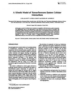
The Celada and Seiden model is a model of a lymph node. It simulates the interactions between lymphocytes, APCs, antibodies and antigen. The lymph node is represented by a two dimensional, four connected grid of sites with periodic boundary conditions (see figure 2.1). Time, space, cells and molecules are discrete. Each site contains a number of cells and molecules, which interact with each other. The behaviour of the system emerges from interactions between cells and molecules. Besides the lymph node, three so called peripheral components are present in the Celada and Seiden model. They represent the bone marrow, the thymus and the environment. They bring new lymphocytes and antigen into the lymph node. In contrast to the lymph node, peripheral components are not modelled after reality. The model aims at realistic modelling the lymph node, so the internal operation of the peripheral components is not important. The model is inspired by cellular automaton theory and shares the following properties with a (generalised) cellular automaton.
20
Peripheral Components Bone Marrow
B cells Lymphnode
T cells
Thymus
Environment
Selected T cells
Antigen
Figure 2.1: An overview of the Celada and Seiden model. The lymph node is the main component. It is modelled as a grid of sites. The bone marrow, thymus and environment are black box modules called peripheral components. They generate B-cells, T-cells and antigen. • Time, space and matter are all discrete • The state space is finite • The dynamics is driven exclusively by interactions between the entities of the automation • The dynamics is probabilistic • Entities have internal dynamics However, it also differs from the traditional cellular automaton in a number of ways. • sites contain multiple entities • entities can step to neighbour sites • interactions are restricted to entities on the same site, instead • not all entities have an internal state The cellular automaton-like way of modelling was chosen for two reasons. The first reason is that because of the cellular automaton-like approach, the model can be described in biological terms rather than mathematical terms. This makes it easy to interpret the results obtained by simulations.
21
B A
T
A
APC
B
T B
B cell
A
A
A
B T
T cell
B
T T
Antibody
B A
B T
T
Antigen
Figure 2.2: A grid site contains a number of entities. Cellular entities are modelled as individuals, molecular entities are modelled as amounts. The second reason is that it makes changing the complexity of the system possible without the need for introducing new qualitative difficulties. When adding a new component, one does not have to change anything in the interactions already present. This makes the system modular and easily extendible.
2.2
Contents of a Site
Figure 2.2 is a close up view of four sites of a lymph node. Each site contains a number of entities: lymphocytes, antigen, antibody and antigen-antibody complexes. The Celada and Seiden model divides the entities into two groups, cellular and molecular entities. The group of cellular entities (or cells) consists of Bcells, T-cells, plasma cells and APCs, as shown on figure 2.3. Cells are tracked individually through the simulation. Each cell has its own age and several other properties. Antigen, antibody and antigen-antibody complexes (figure 2.4) are molecular entities or simply molecules. They are modelled as quantities. At each site, only the amount of each possible antigen, antibody and complex is stored.
22
Receptor
APC
B
MHC
MHC
Receptor
T
Figure 2.3: A schematic picture of an APC, a B-cell and a T-cell. B- and T-cells have a receptor, APCs and B-cells have MHC on which they present antigenic determinants.
Figure 2.4: A schematic picture of antigen and antibody in the Celada and Seiden model. Antigenconsists of a number of epitopes and peptides, each represented by a bit string. Antibody consists of a fixed Fc region and a variable paratope. The Fc region is identical for all antibody, the paratope is an antigen specific receptor.
Properties Receptor∗ , bound antigen∗ , MHC-peptide complex∗ , activity indicator: free or bound, state: virgin or memory, age Receptor∗ , age Receptor∗ , state: virgin or memory, age MHC-peptide complex∗ , activity: free or bound One or more epitopes∗ , one or more peptides∗ Paratope (variable)∗ , peptide (fixed)∗ One or more antigen peptides∗ , antibody peptide∗
Table 2.1: The properties of cells and molecules as represented by the Celada and Seiden model. Properties marked ∗ are represented by bit strings. The other properties are state or activity indicators.
2.3
Diffusion
Figure 2.2 shows four neighbour sites in the grid. Each simulation time step, entities are allowed to diffuse to a direct neighbour through the grid. Diffusion of entities is the only way of interaction that exists between different sites in the grid. The diffusion of cellular entities is computed using a random walk algorithm. Each time step, they step to a random neighbour site, or stay at the same site. For molecular entities, the random walk algorithm is not used. Instead, the number of molecules that diffuses to each neighbour is obtained by equally distributing the molecules to the four neighbour sites.
2.4
Entities
The Celada and Seiden model discriminates between cellular and molecular entities. Table 2.1 lists the entities of the Celada and Seiden model and their properties. The following properties in this table represent proteins: the receptors of B-cells, plasma cells and T-cells, the MHC-peptide complex of B-cells and APCs, the epitopes and peptides of antigen, the paratope and peptide of antibody, and the peptides of an antigen-antibody complex. In the Celada and Seiden model, these proteins are all represented bit strings.
2.4.1
B-cell
Each B-cell has a receptor for recognising antigen, as shown in figure 2.3. When a B-cell encounters antigen, the affinity between the B-cell receptor and the epitopes of the antigen determines whether the B-cell binds to the antigen. If a B-cell has bound to antigen the bound antigen property of the B-cell refers to the antigen. The B-cell presents parts of an antigen peptide together with MHC as an MHC-peptide complex. B-cells have an activity indicator, which shows whether a B-cell is free or has bound antigen. A state indicator indicates whether a B-cell is a memory or a 24
virgin cell. Age is a special variable, determining whether a B-cell is proliferating. If a B-cell becomes stimulated, its age is reset to zero. This makes the B-cell proliferate, until its age reaches a certain threshold.
2.4.2
Plasma Cell
Plasma cells are a special kind of B-cells that are not able to recognise antigen themselves. Instead, they produce large amounts of antibodies that are able to recognise and bind to antigen, and form antigen-antibody complexes. Antibody have a paratope that is identical to the receptor of the plasma cell that produced them.
2.4.3
T-cell
T-cells have a receptor that allows them to recognise MHC-peptide complexes. Like B-cells they can be virgin or memory, and they have an age which determines whether the cell is proliferating.
2.4.4
APC
APCs recognise antigen-antibody complexes with a high affinity, and antigen with a very low affinity. They perform non-specific antigen recognition. They can be either free, or bound to an antigenor antigen-ab complex. Like B-cells, they present antigenic determinants together with MHC as an MHC-peptide complex.
2.4.5
Antigen
Antigen is represented by a number of proteins. Each antigen has one or more epitopes and one or more peptides, represented by bit strings. Figure 2.4 shows a schematic picture of how antigen is represented in the Celada and Seiden model. Epitopes and peptides are represented by bit strings. Epitopes are recognised by B-cell receptors and antibody paratopes.
2.4.6
Antibody
Antibody consists of a variable paratope, identical to the receptor of the plasma cell that created it and a fixed peptide, the Fc region. The Fc region, which is identical to all antibody, is recognised by APCs and allows APCs to bind antigen-antibody complexes.
2.4.7
Antigen-Antibody Complexes
An antibody that binds to an antigen form an antigen-antibody complex. A complex has the following properties. The variable parts the epitope of the antigenand fixed part the antibody Fc region. 25
Antigen
Receptor
B MHC
Figure 2.5: The B-cell-receptor and the epitope of the antigen match perfectly, because the antigen epitope exactly complements the B-cell receptor.
2.5
Computing the Affinity
In the Celada and Seiden model, two affinity functions are present. The first function, which is discussed in section 2.5.1, is mainly used when computing the affinity of a receptor and an epitope or MHC-complex. The second function, discussed in 2.5.2, is mainly used when the affinity between MHC and peptides is computed. In both functions, the affinity is a function of the number of mismatches between two bit strings. A bit string may represent a receptor, an epitope, a peptide, an MHC or a MHC/peptide complex. A perfect match of two bit strings happens when the strings have a complementary value at each position, as shown in figure 2.5. The mismatch of two bit strings is defined as the number of bit positions at which the two bit strings have an equal value. The example has a mismatch of 0, while two strings containing the same values have a mismatch equal to the bit string length.
2.5.1
Receptor Affinity
The main affinity function is the one described in this section. Throughout the rest of the paper, this function will be referred to as T (r, e), where r and e are two bit strings, in most cases a receptor and an epitope. To compute the affinity between two arbitrary bit strings r and e, the only thing we need to know is the number of mismatching bits, or simply the mismatch. Once the mismatch x of the tuple (r, e) is computed, the affinity level S(x) is a floating point number in the interval [0, 1]. For perfect matching strings, the matching strength is always 1. Bit strings with a mismatch larger than the maximum allowed mismatch M have a matching strength of 0. The affinity level that corresponds to to the maximal mismatch is a system parameter l The remaining affinity values for all mismatches are now recursively computed from l and an affinity enhancement factor a and the bit string length n, in the following way.
26
S(0) = 1 S(M ) = l S(i − 1)
=
(2.1)
¡n ¢ min(S(i)a ¡ ni ¢ , 1) i−1
¡ ¢ In this equation, ni denotes binomial coefficients. The reason to include binomial coefficients into the formula for computing affinity is that the number of possible cells with a mismatch of i corresponds binomially, relative to n, with the value of i. As an example, in a 8 bit system, the number of perfect matches is one, the number of 1-bit mismatches is 8, the number of two-bit mismatches is 28 and the number of possible three-bit mismatches is 112. By including binomial coefficients into the affinity level formula, it is accomplished that the probability that an i-bit mismatch will lead to a binding is a times lower than the probability that a i + 1-bit mismatch will lead to a binding. A more precise explanation for the affinity level computation can be found in [11, section 4.2].
2.5.2
MHC Affinity
A different affinity is the affinity that is used in binding peptide to an MHC groove. This affinity will be called U (m, c) throughout the rest of the paper. The main difference is that the maximal allowed mismatch doesn’t apply here. For bit strings m and c with a mismatch of x the formula is defined as follows. 1 S(x) = ( )x 2
(2.2)
This affinity function is used in section 2.7.2 and section 2.8.2.
2.6
Interactions
The behaviour of the model lymph node emerges from the interactions between the entities. The interactions can be divided into three types: cell to cell interactions, cell to molecule interactions and molecule to molecule interactions. In the next section, the events that happen during an immune response is summarised. Later sections describe the interactions in more detail, in the order they occur in the simulation.
2.6.1
Cell to Cell Interactions
The following cell to cell interactions are allowed in the Celada and Seiden model.
27
• T-cell - B-cell interaction • T-cell - APC interaction B-cells or APCs that have bound an antigen or antigen-antibody complex can interact with T-cells. The cell to cell interaction operates as follows. The APC or B-cell presents an MHC-peptide complex to the T-cell. The affinity between the T-cell receptor and the complex serves as the probability that the T-cell interact with the B-cell or APC. Section 2.5 explains exactly how the affinity between a T-cell and a B-cell or APC is computed. If interaction takes place, the following happens. • The age of the T-cell and the B-cell or APC is reset to 0, marking them as stimulated and allowing the T-cell and B-cell to proliferate • Antigenic peptide is removed from the MHC-peptide complex on the APC or B-cell • If the T-cell or B-cell was a virgin cell, it is promoted to a memory cell. Because APCs do not divide in this model, their stimulation only prevents them from interacting with other T-cellsduring the current time step.
2.6.2
Cell to Molecule Interactions
In principle, all three types of molecules can interact with B-cells and APCs, which gives six types of cell to molecule interactions. APCs perform non-specific recognition. antibody or antigen-antibody complex have each a predefined affinity to APC, which is unrelated to the receptor or epitope values of the molecule. The affinity of a B-cell with a molecule type consists of a base affinity, adjusted to the number of molecules on the site and the affinity between the B-cell receptor and the molecule. This is explained further in the section on affinity, 2.5. If the affinity between the cell and molecule is high enough, the cell constructs an MHC-peptide complex, consisting of the left half of the MHC and the right or left half of one of the peptides.
2.6.3
Molecule to Molecule Interactions
The only example of molecule to molecule interaction is the formation of complexes through interaction between antigen and antibody. Because molecules are handled as quantities instead of as individuals, their interactions are solved numerically. For each combination of antigen and antibody available in the system, the affinity is computed. Multiplicating the affinity with the minimum of the number of antigen and antibody yields the number of complexes that would form, if only one type of antigen and antibody would be in the system.
28
Antigen B−cell binds
Receptor
antigen
B MHC
B−cell processes antigen and presents antigenic determinants
Receptor
T−cell binds to
Receptor
B−cell and releases lymphokine
After the proliferation cycles, Plasma cells will produce large amounts of antibody.
B MHC
B
Several division cycles result in a clone of B−cells, plasma cells and T−cells
Receptor
Receptor
Receptor
B
Plasma
T
Receptor
Receptor
Receptor
B
Plasma
T
MHC
MHC
Receptor
T
MHC
Figure 2.6: A summary of the events happening during an immune reaction. For each combination of antigen and antibody the above quantity is computed at each site. These quantities are adjusted to the total number of antigen and antibody available, so the total number of bindings does not exceed the number of molecules of a type available.
2.6.4
Immune Reaction
Figure 2.6 shows the process of an immune reaction in a schematic representation. In the simulation, the immune reaction displayed here takes several time steps to complete. The process starts after antigen has been injected into the system. A B-cell whose receptor has a high enough affinity with one of the antigen epitopes binds the antigen. The activity indicator changes from free to bound. The B-cell processes the molecule and presents antigenic peptides together with MHC as an MHC-peptide complex. An MHC-complex is constructed by taking an MHC bit string, and replacing the right half of that string by either the right or the left half of one of the peptides of an antigen. Which peptide half is used, is determined in the following way. For each of the
29
peptide halves, the affinity with the right half of the MHC is computed. The peptide with the best matching peptide half is chosen. The right half MHC binds the peptide half it has the highest affinity to. The other peptide half becomes the right half of the MHC-peptide complex. For computing the affinity of two protein halves, the function U (m, c) from section 2.5 When a T-cell whose receptor matches with the MHC-peptide complex stimulates the B-cell and itself to proliferate by releasing cytokine. At this point, the age of both the B- and T-cell is reset to 0 and the state of both cells changes from virgin to memory. this makes both cells long lived, and constitutes the memory effect. Stimulated B- and T-cells start to proliferate and after several division cycles, the B-cells undergo one final division cycle into a B memory cell and a plasma cell. Plasma cells now produce high amounts of antibody, that recognise the antigen that initiated the process described here. The antibody now form complexes with the antigen. Antigen-antibody complexes are recognised by APCs, and are digested. The APCs ingest the complexes, and present parts of the peptides of the complex (which are still antigen peptides) together with MHC on their cell membrane. After a time step finishes, the APCs are reset, and are able to bind new complexes.
2.7
A Time Step in Simulation
The previous section gave a summary of what happens during a number of time steps. In this section, we discuss the events of the simulation in the order in which they occur during a time step, as shown in figure 2.7.
2.7.1
Reset and Initialise
At the start of each time step, the activity of B-cells and APCs is reset as follows. The activity indicator of each APC is reset, so the APC is ready for binding. B-cells are reset too, except when they are currently in a division cycle.
2.7.2
T/B-cell and T-cell/APC Interactions
After the reset of B-cells and APCs, the simulation continues with the cell to cell interactions. B-cells and APCs presenting antigenic determinants together with MHC on their cell membrane are bound and stimulated by T-cells in this event. There may exist several binding possibilities for a T-cell, because multiple Bcells and APCs presenting antigenic determinants may exist at a single site. T-cellsare allowed to bind only one B-cell or APCat a time, so conflict resolving is needed. Therefore, two lists of possible bindings at the site are created and sorted on basis of matching strength. The list are created in the following way: 30
Start of Timestep End of Timestep
Reset and initialize cells T/APC and T/B−Cell Interactions
Output data
Inject new antigen
Cell Decay
Diffuse entities across grid
Interactions between cells, ag and ab
Create
Molecule decay
antibodies Proliferation and mutation of cells
Figure 2.7: A time step in simulation
31
• randomise the order of the T-cell list and the B-cell or APC list. • traverse the list of T-cells available for binding and compute the affinity between the current T-cell and all APCs or B-cells available for binding. • The computed affinity serves as a probability for adding the pair to the possible bindings list (see 2.5 for details on computing the affinity). • When a pair has been added to a possible bindings list, neither of the cells can be added to that same list of possible bindings again. This last step resolves the problem that a T-cell may be able to bind to several APCs or to several B-cells at the same time. However, a certain T-cell may still occur in both the T-cell - APC and in the T-cell - B-cell matches list. The complete algorithm is thus as follows. • Create a list of possible T-cell - APC bindings, each item consisting of a T-cell index and a APC index • Create a list of possible T-cell - B-cell bindings • Sort the two lists by the T-cell index • Concurrently traverse the two lists of possible matches. When a T-cell occurs in both lists, remove one of the possible matches at random. • All conflicts are resolved. The final step is to execute all bindings that are left in the list of possible matches. This procedure is repeated at each site in the system. Now, each T-cell has had the opportunity to interact with each APC and B-cell at the site.
2.7.3
Cell Decay
Cell death is simulated by removing cells from the system. All types of cells are assigned a certain half-life τ . The probability P that a given cell survives the time step is then derived according to this formula. P = e−
ln 2 τ
(2.3)
Memory B- and T-cells usually have a half-life of 50 time steps, while virgin Band T-cells only have a half-life of 10 time steps. Decay of antigen, antibody and complexes occurs at a later stage in the time step, according to the same decay formula.
32
2.7.4
Molecular Interactions
At this point, interactions involving molecules are executed. The Celada and Seiden model has the following types of molecular interactions: • antigen - antibody interaction • antigen - APC interaction • antibody - APC interaction • antibody-antigen complex - APC interaction • antigen - B-cell interaction • antibody - B-cell interaction • antibody-antigen complex - B-cell interaction In reality, these interactions occur at the same time. In the model, it is not possible to have all different interactions occur simultaneously. As a compromise, these interactions happen in a different, random order at each site. Because the different interactions have a lot in common, we introduce the notion of agents and targets. B-cells, APCs and antibody are called agents, antigen and complexes are called targets. A target type denotes all targets with the same molecule type. All antigen at a site is a target type. Specific target type denotes all targets of a type having the same specificities. As an examples, all antibodys with the same receptor are a specific target type while the collection of antibodywith every possible receptor is a target type. Finally, the specific target concentration denotes the concentration at one site of a specific target type. Whether an agent a binds a target t depends on the affinity A(a, t) and the concentration of the target. The affinity can be seen as the probability that a binding would occur, provided no other agents or targets are available. The interaction strength IS is the binding probability of an agent a and a target t, where the concentration of t is c. This is expressed in formula 2.4. IS(a, t) = 1 − (1 − A(a, t))c
(2.4)
This is the general formula, which is used in both APC-target binding and in B-cell-target binding. When computing the probability that an APC binds a target type, we can lump together all specific target types. This is possible, because the affinity between the APC and each of the specific target types is equal. The probability that the current APC binds to any target of the the current target type is equal to the interaction strength defined in formula 2.4. Before the APC can be bound however, a specific target type has to be chosen. The relative concentrations of the specific target types serve as a probability that the specific target type is bound by the APC. The summarised algorithm for APC-target binding is: 33
• Compute IS(a, t) using formula 2.4 • Traverse the list of agents, let IS(a, t) serve as the binding probability • If a binding occurs, choose a specific target type according to the concentration distribution, make the APC unavailable for binding and decrease the concentration of the current specific target type Computing the probability that a B-cell will bind antibody or an antigen antibody complex works similar, but is more complicated, because the receptorspecific affinity has to be taken into account. Formula 2.4 is still valid for each specific target type, but lumping together specific target types is impossible. Another small complication is that an antigen possibly has different epitopes. This is overcome by treating a multi epitope antigen like multiple single epitope antigens. This gives B-cells the opportunity to interact with all epitopes the antigen carries. A modified algorithm that ensures that these differences are dealt with is the following. • For each combination of bindable B-cells and specific target types • The affinity IS(a, t) serves as a binding probability • If a binding occurs, make the B-cell unavailable for binding by marking it as stimulated, promote the B-cell to a memory cell, and decrease the target concentration An agent that has been bound once, is unavailable for binding until it is reset at the start of the next time step. In this process, combinations tried first have a higher probability of succeeding than matches that are tried later on. This problem is solved by traversing the agent and target lists in a random order. The intermolecular interactions are those between antigen and antibody. A successful binding between an antigen and antibody will result in their respective concentrations to decrease and the concentration of complexes to increase by one. Because both antigen and antibody are listed as concentrations, we use a modified version of equation 2.4 to determine the number of bindings that will occur for a given combination of antigen and antibody. For each specific type of antigen i and for each specific type of antibody j with concentrations ci and cj , the number of bindings B(i, j) that will occur is defined as follows.
Using equation 2.5 it is now possible to compute the number of bindings between i and j that would occur provided no other types of antigen or antibody would exist. The algorithm for antigen antibody interaction can now be summarised as follows. 34
• Traverse the list of combinations of antigen and antibody in a random order • For each antibody i and each antibody j, remove B(i, j) antigen and antibody from the lists, and add B(i, j) complexes to the list of complexes of type j. Like the algorithms for binding cells to molecules, this algorithm solves the problem of conflicting bindings in a simple and transparent way.
2.7.5
Decay of Molecules
Antigen, antibodies and complexes are subject to decay, just like cells. Decay occurs according to the survival rate function mentioned in 2.7.3. The half-lives of antigen, antibody and complexes are model parameters. For antigen, this decay can be inverted by a multiplication agent, simulating a chronic infection.
2.7.6
Cell Population Growth
Each time step, new B- and T-cells cells are added from the bone marrow and thymus, to compensate for dying cells. These new virgin cells have survived the selection routines that prevent self reaction. The number of cells n added is derived from the initial population size I and the half life τ of the cell in question, analogously to computation of survival probability. n = I ∗ (1 − e−
ln 2 τ
)
(2.6)
Not all new lymphocytes enter through the peripheral components. Stimulated B- and T-cells will proliferate into two new cells. During the final cell division, B-cells will divide one more time into a plasma cell and a B memory cell. During a number of divisions, the receptor of B-cells may hypermutate (see 1.2.11). This hypermutation is simulated by randomly flipping one or more bits of the receptor of the daughter cells. The mutation probability is a system parameter. Hypermutation occurs during the first n or the last n division steps, controlled by a system parameter. If hypermutation occurs, the B-cell population will no longer have identical receptors. Some B-cells have a mutated receptor with a higher affinity to the antigen better then their parents receptor. These mutated B-cells recognise antigen with a higher probability and thus a higher growth rate. Other mutated B-cells have a lower affinity. They will have a lower or probability of recognising the antigen, and their growth rate will be much slower. This mechanism results in a bootstrap toward a clone of B-cells with high affinity receptors.
2.7.7
Diffusion
One of the final processes of a time step is diffusion. While interactions occur only between entities on the same site site, entities can move to a neighbour site every time step. The diffusion rate is a system parameter. 35
2.7.8
Injection of Antigen
At a number of time steps, antigen is injected into the system. This is simulated by increasing the antigen concentration lists. Parameters controlling the injection of antigen are the time of injection, amount of antigen to be injected and the specificity of the antigen. The antigen can be injected at one single site, or spread equally across the system.
2.8
The peripheral components
In the Celada and Seiden model, the peripheral components act like black box modules. In this section their operation is explained.
2.8.1
The Bone Marrow
In the bone marrow, a constant stream of B- and T-cells is generated, compensating for dying cells. Creating a new cell in the bone marrow can be summarised as follows. • Generate a new cell with a randomly chosen receptor • Assign an MHC to B-cells For the purpose of testing the effectiveness of hypermutation, it is possible to exclude a range of B-cell receptors. The exclusion makes it possible to guarantee that no high affinity B-cells are in the system when the antigen is introduced. If, after a number of time steps, high affinity B-cells appear in the system, the effectiveness of hypermutation is proven. The exclusion works by inserting a gap into the repertoire of B-cell receptors. The effect is that all B-cells have a certain minimal mismatch to any antigen introduced during the simulation. High affinity B-cell receptors are not available, so the system will have to bootstrap itself from low affinity B-cells.
2.8.2
The Thymus
The T-cells created in the bone marrow have an arbitrary receptor. Some Tcells will therefore be able to recognise self proteins. This self recognition leads to self immune diseases. The thymus module prevents self immunity by eliminating self reactive T-cells before they enter the lymph node. This process is called thymic selection. In this model, the thymus function is not a realistic module, nor does it comply to the cellular automaton rules. Instead, a numerical solution is used for selecting only receptors that are not self reactive. This selection consists of tree steps. • Positive selection for complementarity with parts of at least one MHC.(S 1 ) • Negative selection for complementarity with any bare MHC.(S2 ) 36
• Negative selection for complementarity with any MHC loaded with self peptides.(S3 ) In order to survive thymic selection, a receptor must survive all three selection steps. The total survival probability is consequently the product of the probabilities S1 , S2 and S3 . To mimic the properties of a dense organ like the thymus, these selection steps are applied a number of times n. The total selection probability S is thus defined as follows. S=(
3 Y
Si )n
(2.7)
i=1
The survival probabilities for all receptors are stored in an array. While this array can be very large (2n for bit string size n), it is also very sparse. Most values have a probability of exactly 0, due to the strict combination of positive and negative matching. Therefore, only the nonzero values are stored. The problem of selecting a receptor for a new T-cell is now reduced to the following procedure. • Select at random a receptor from the list of receptors with non-zero survival probabilities. • Decide if this receptor is to be chosen on basis of the survival probability of the receptor. • Continue this procedure until a receptor is accepted. Before the simulation starts, a hash table is created of all allowed receptors and their probabilities. This is done in the following way • Compute the survival probability p for each possible receptor r • if p > 0, add the tuple (p, r) to the list of allowed receptors. When this list is created, selecting T-cell receptors is possible in a fast and simple way. Complementarity with MHC A B-cell or APC presents antigenic determinants together with MHCon its cell membrane. The affinity of a T-cell with receptor r and such a complex c is T r, c, where T is the affinity function explained in section 2.5. The complex presented by APCs and B-cells consists of the left half of the MHCand either the left or right hand or the antigenic peptide. The T-cell can only bind to a MHC-peptide complex, if it has a positive, nonzero affinity to the complex. A process called positive selection eliminates all T-cells that don’t have a minimal affinity to the left half of the MHC. These T-cells would never be able to bind a complex, and are thus useless. 37
The left half of each T-cell receptor must have a mismatch of at most the maximal defined mismatch with the left half of any of the MHC. If the left half of a receptor has a mismatch of more than the maximal mismatch, S1 for that receptor will be 0, otherwise it will be 1. If S1 = 0 for a receptor, the product of S1 , S2 and S3 will be 0, and the receptor is not added to the list of receptors with a positive survival rate. Binding of MHC without Peptide B-cells and APCs that have not bound a molecule, will present a complete MHC bit string. T-cells that have affinity to this bare MHC, are self reactive. They will stimulate cells that present MHC without a antigenic determinant. The second selection, S2 , eliminates receptors r that recognise bare MHC m. Y S2 = (1 − T (r, m)) (2.8) M HC
As this equation shows, if the affinity a for a T-cell is in the range 0 < a < 1, it is still possible that the T-cell receptor is accepted. This means that T-cells with some affinity can be accepted. Affinity with MHC/self peptide complex This is the most complex selection step. The purpose is to prevent T-cell receptors that have affinity with MHC loaded with self peptides from being selected. To compute S3 for a given receptor r, the affinity of r to every possible complex of MHC and self peptide are computed. An MHC m and a self peptide p can be bound into one complex in two ways as follows. The left half of the complex is always the left half of of the MHC. The right half of the MHC will be bound to one peptide half. Consider the complex c, which has the left of MHC m as a left half cl , and the left half of self peptide p as its right half cr . This peptide is created by binding the right half of p, pr to the right half of the MHC m, mr . This makes cl = ml , and cr = pl . The affinity α(r, c) is now expressed by α(r, c) = T (mr , pr )U (r, c)
(2.9)
where U is the affinity function discussed in section 2.5. S3 is now computed as follows. Y (1 − (α(r, c)) (2.10) S3 (r) = c
Summarising, the first selection (S1 ) is an all-or-nothing selection. The latter two are survival probabilities, so some T-cell receptors are accepted at times and rejected at others. The result is a T-cell receptor population where self reactive T-cells are unlikely to have a high concentration, but will occur occasionally. This reflects reality, where self reactive T-cells can occasionally get into the immune system, without having large impact unless the individual is suffering from a self immune disease. 38
2.8.3
Injection of Antigen
An antigen injection is specified by the following variables. • A list of epitopes and peptides the antigen consists of • The time at which this dose of antigen is to be injected • The amount of antigen that is to be injected • The antigen can be injected at one grid point or dispersed across the grid At times specified by the experimenter, antigen is added to the lymph node in the following way. • If the specific antigen has not been injected before, add the antigen to the list of antigen descriptions. • If the antigen is to be dispersed, equally distribute the amount of antigen across all grid points. • If the antigen is to be injected at a single point, increase the concentration at a single point. Antigen can be injected into the lymph node at any time. Injections of different types of antigen at the same time are allowed.
2.9
Simplifications
The model used in this project is a simplified version of the one by Celada and Seiden. The model was implemented using published work by Celada and Seiden and the Immsim manual by Olivier Lef´evre [11]. This manual contains a description of the original APL2 implementation by Celada and Seiden in 1992. The next sections briefly discuss the simplifications we made.
2.9.1
Anergy
A phenomenon observed in immunology is anergy. Anergy is believed to be a control mechanism, preventing self immunity or unlimited B-cell proliferation. When a B-cell is surrounded by many activated B-cells, it becomes anergic. Anergic B-cells are unable to bind antigen. The original Celada and Seiden model implements this phenomenon. The effect, however seems to be measurable only in some extreme cases and not important for the general functioning of the model [11, section 6.8]. Therefore, the effect of anergy was not included in this implementation.
39
2.9.2
Grid
The original implementation uses a triangular, six connected grid. We used a four connected grid instead. All publicised simulations use a diffusion rate of 1. Pattern formation is not discussed in any of the publications.
40
Chapter 3
Simulation Results Celada and Seiden have published the results of a their simulations in a number of articles [12, 2, 3]. The tests involved simulating phenomena observed about the immune system, comparing the results to the results of in vivo or in vitro and analysing them to see if theories proposed by immunologists explain the phenomena in the simulations. The simulation program we implemented is based on the Celada and Seiden model. To test the correctness of our implementation, we repeated the experiments published by Celada and Seiden.
3.1
Initial Results
The initial publication of the Celada and Seiden model in [12] included the discussion of a number of simulations with the Celada and Seiden model. From the outcome of these simulations it was concluded, that the system performed reasonably like a real immune system. Our first goal in testing our implementation was reproduction of the results published in [2]. In our first experiment, we injected antigen at time steps 5 and 45, in a system with bit string length 8, an initial population of 1000 APCs, B-cells and T-cells on a grid of 15x16 sites. Figure 3.1. After the first injection, it takes a while before the populations of B- and T-cells start to grow, and it takes almost thirty time steps, before the antigen has disappeared completely. After the second injection, only very little B-cells bind antigen, due to the high concentration of antibody. The antibody graph shows a sharp decrease of almost 500, immediately after the second injection. The amount of antigen immediately drops to zero. The results in figure 3.1 are comparable to that of the original publication. Figure 3.2 shows the mean and standard deviation of the B memory cell population over 15 simulation runs, each started with a different random seed. (The differences between simulation runs are within reasonable bounds.)
41
350
500 450 400 350 300 250 200 150 100 50 0
T memory 300 250 200 150 100 50 0 0
50
100
150
200
250
antigen
0
200
50
100
150
200
250
7000 B memory
Total antibody concentration 6000
150
5000 4000
100 3000 2000
50
1000 0
0 0
50
100
150
200
250
0
50
100
150
200
250
Figure 3.1: Antigen is injected at time steps 4 and 45. At the time of the second injection, a lot of antibody is still available, binding most of the antigen. A small number of B-cells bind antigen, accounting for the small second peak in B memory cell population. 300 B memory cells
250
200
150
100
50
0 0
50
100
150
200
250
Figure 3.2: Development of the B-memory population. Error bars show the standard deviation over 15 simulation runs.
42
3.1.1
Immunisation
We did a series of tests, in which the time of the second injection was varied. The second injection occurred at time step 45, 65, 85, 105, 125 or 175, and we repeated each test with 15 different random seeds Figure 3.3 shows the maximal level of antibodies that is reached after the second injection. If antigen is injected before most antibody has disappeared, most antigen is bound by antibody, and the highest level of antibody seen after the secondary injection is still due to the primary response. This happens in the tests were antigen is injected at time step 85 or earlier. If most of the antibody has disappeared at the time of the second injection, the secondary response is higher than the primary response. If, however, the number of B memory cells has started to decrease, the second response is slower. The maximal response occurs if antigen is injected for the second time at time step 125.
3.1.2
Antigen Dependency of the Immune Response
In another series of 25 experiments we randomly varied the antigen specificity. We injected a small amount of antigen at time step 5 and time step 105, and used a random antigen in each test. In general, the system responded with first response, followed by a higher secondary response. Some antigen, however, was not recognised well by the system. Figure 3.3 shows the response of one such test. Further testing with these antigen specificities revealed that the MHCcomplexes presented by B-cells are bound by only very few T-cells. As a result, the number of B-cells that proliferates is very low. The antigen we used in this experiment consisted of one epitope and two peptides. A 1-bit change in one of the peptides of the antigen was sufficient to get a normal response, comparable to other experiments. A probable explanation for this case is that the most common MHC-complexes were not recognised by T-cells, because the complexes had a lot in common with normal body MHC. As said, in general the responses were as expected. Figure 3.5 shows the mean and standard deviation of the B memory cell response in the 25 runs we did. Because of thymic selection, not every antigen is recognised as fast and as easy, which leads to a large standard deviation.
3.1.3
Priming
We did a small series of experiments, in which the only parameter varied was the dose of primary and secondary antigen injection. As doses we used 10, 100, 1000 and 10000, both for the primary as for the secondary response.
43
25000 Total amount of antibodies High affinity antibodies Low affinity antibodies 20000
15000
10000
5000
0 40
60
80
100
120
140
160
180
Time of second antigen injection
Figure 3.3: The highest level of antibodies reached after the second antigen injection as a function of the time of the second injection. If the second injection occurs before time step 100, some antibody is still available and not all antigen will be bound by B memory cells, lowering the secondary response. As the time between the two antigen injections becomes larger, fewer B memory cells will be available at the time of binding, resulting in a decreasing second response if the antigen was injected after time step 130.
44
160
300 T memory
140
antigen 250
120 200
100 80
150
60
100
40 50
20 0
0 0
50
100
150
200
250
0
35
50
100
150
200
250
900 B memory
Total antibody concentration
800
30
700 25
600
20
500
15
400 300
10
200 5
100
0
0 0
50
100
150
200
250
0
50
100
150
200
250
Figure 3.4: While most antigen was adequately recognised, this is an example where the model gave a very uncommon response. Apparently, antigen is recognised by B-cells, but T-cells hardly stimulate any bound B-cells. The response is slow and ineffective.
3.2
Increasing the Bit String Size
In the first publications by Celada and Seiden, receptors, peptides, paratopes, and epitopes were represented by bit strings of length 8. While Celada and Seiden were able to generate some interesting results with this system, the diversity in an 8 bit system is very small. Experiments published later use a bit string of length 12 for every protein in the system, allowing a diversity of 4096. Although this still low when compared to the diversity of a real immune system, a number of interesting experiments that can not be done using an 8 bit system, can be simulated in a 12 bits system. For some experiments, larger bit strings may be required. Many parameters turn out to depend on the bit string length. Increasing the bit string length implies that some parameters have to be adjusted, most notably the following. The following sections explain which parameters depend directly or indirectly on the bit string size, and have to be adjusted when the bit string length is changed.
3.2.1
Maximal Allowed Mismatch
In an 8-bit system, only perfect matches and one-bit mismatches are allowed. The probability P of a m-bit mismatch in a n is given by the following formula,
45
600 B memory cells
500
400
300
200
100
0 0
50
100
150
200
250
Figure 3.5: This figure shows the mean B-cell response and its standard deviation, when exposed to 25 random antigen. The standard deviation is large because some antigen are more easily recognised than others. Figure 3.4 shows an example of one of the antigens that was hardly recognised by the system.
P (m) =
¡n¢ m
2n
(3.1)
¡n¢ n! = m!(n−m)! where m . For an 8-bit system, this means that the probabilities of a perfect match and a 1-bits mismatch between a B-cell and an antigen epitope 1 8 are respectively 256 ≈ 0.004 and 256 ≈ 0.020. The maximal mismatch being 1, this means that approximately 2.4% of all B-cells in the system have some affinity to the antigen. When increasing the bit string length to 12, these numbers change dramatically: the probability of a perfect match between two bit strings has dropped to about 0.0002, and a one-bits mismatch has a probability of 0.0029. This means that no significant immune response will happen, unless the maximal mismatch is increased. Therefore, in all 12-bits experiments, the maximal allowed mismatch is set to 3. This increases the probability of a nonzero affinity between two arbitrary bit strings to 0.073.
3.2.2
Affinity Level
The affinity level a system parameter that defines the affinity between two strings that have the maximal allowed mismatch. Because the affinity of two
46
bit strings is recursively defined from the affinity level and the number of mismatches between the two strings (see section 2.5), the affinity level must be adjusted if the maximal number of allowed mismatches is changed. The affinity function A(m) is defined as ¡ n ¢ ¡n¢ A(m) = A(m + 1)a m+1 m
n (m+1 ) compensates for the binomial distribution of mismatchn ( m) ing bit strings. Because of this compensation, the probability that an m-bits mismatch leads to a binding is a times larger than that of an m + 1-bits mismatch. A problem is now that the probability reaches 1 too quickly if the affinity level is set too high. In the case of a 12-bits system, a 2-bit mismatch is more likely to occur than a 1-bits mismatch if the affinity level isn’t lowered sufficiently. Therefore, when increasing the maximal mismatch, an appropriate low value for affinity level has to be chosen.
In this function,
3.2.3
Population Size
As the B-cell receptor repertoire increases exponentially with the size of the bit strings, the probability that a B-cell has enough affinity to bind an antigen decreases very fast. This is partly compensated for by increasing the maximal allowed mismatch, but that alone is not good enough. Therefore, it is necessary to increase the population sizes of B- and T-cells and APCs.
3.2.4
Grid Size
Increasing the cell population sizes has the side effect of increasing the number of cells on one site. Because a site represents the same geometric space unrelated to the number of cells in the system, it is reasonable to increase the number of sites when the population increases.
3.2.5
Number of Time Steps Simulated
An effect we observed in our simulations, was that more time steps passed, before a response occurred. This is due to the lower total affinity of the system after right after the first immunisation, and is an effect visible in the results published in [3]. Figure 3.6 and 3.7 show two identical experiments with a different bit string size. Clearly, the immune response is much slower in the 12-bits simulation. Still, the second response is quicker, and leads to a faster growth. Delaying the second antigen injection until time step 175 for the 12-bits system, results in a stretched version of figure 3.6.
47
800
500 450 400 350 300 250 200 150 100 50 0
T memory
700 600 500 400 300 200 100 0 0
50
100
150
200
250
antigen
0
700
50
100
150
200
250
25000 B memory
Total antibody concentration
600
20000
500 400
15000
300
10000
200 5000
100 0
0 0
50
100
150
200
250
0
50
100
150
200
250
Figure 3.6: Immunisation: antigen is injected at time steps 5 and 125 in an 8-bit system.
900
600 T memory
800
antigen 500
700 600
400
500
300
400 300
200
200
100
100 0
0 0
50
100
150
200
250
0
350
50
100
150
200
250
7000 B memory
Total antibody concentration
300
6000
250
5000
200
4000
150
3000
100
2000
50
1000
0
0 0
50
100
150
200
250
0
50
100
150
200
250
Figure 3.7: The same experiment as in figure 3.6, now using 12-bit receptor strings. The response is much slower and the second injection happens while there is still some antigen available.
48
Parameter B-cell population T-cell population APC population Grid size Maximal mismatch Affinity level Life time of memory cells Time scale
Table 3.1: Parameters of the Celada and Seiden model that depend directly or indirectly on the length of the bit strings used in the simulations.
3.2.6
Life Time of Memory Cells
Because the time scale is stretched, the half life of B memory and T-memorycells has to be increased, to prevent the population of memory cells from disappearing before the next antigen injection occurs.
3.2.7
Parameters Settings in 8- and 12-bit Simulations
Table 3.1 lists the parameters that are adjusted when the bit string length is increased from 8 to 12. As the table shows, quite a number of parameters turn out depend, directly or indirectly, on the bit string length.
3.3
Affinity Maturation
In a real immune system, the diversity of B-cell receptors is orders of magnitude smaller than the receptor diversity. As a result, after a first infection, the response will be mainly due to low affinity B-cells. Through clonal selection and hypermutation, the immune system is capable of to developing high-affinity B-cells from low affinity B-cells (see section 1.2.11). The Celada and Seiden model simulates both clonal selection and hypermutation. In 1996, Celada and Seiden published the results of their experiments on hypermutation in [3]. Their main conclusions were the following. • In a small repertoire, hypermutation is not necessary to achieve a high population of high affinity B-cells • If the B-cell population is limited, hypermutation is essential for filling the holes in the repertoire • The mutation rate and the affinity enhancement factor are a very sensitive parameters for affinity maturation We did a number of simulations, in which we repeated the affinity maturation experiments of Celada and Seiden. Figure 3.8 shows the mean antibody response
49
25000 Total antibody concentration Perfect matching antibody 1-bits mismatching ab antigen 20000
15000
10000
5000
0 0
50
100
150
200
250
Figure 3.8: Affinity maturation through clonal selection. During the primary response, more low affinity antibody is produced than high affinity antibody. In the secondary response, the opposite happens. This is an effect of clonal selection. of an 8-bit system over 15 simulations, as a result of antigen injection at time step 5 and 125. During the primary response, low affinity (i.e. 1-bits mismatching) antibody is produced in higher quantities than high affinity antibody. During the secondary response however, the amount of high affinity antibody produced is much higher than the amount of low affinity antibody.
50
Chapter 4
Discussion In this chapter, we discuss the questions posed in section 1.4. In section 4.1, we address the questions we posed with regard to the Celada and Seiden model, in section 4.2 we discuss the questions on simulating the immune system for purposes other than immunology. Conclusions are given in section 4.3
4.1 4.1.1
The Celada and Seiden model Reproducibility
The first question we wanted to answer, is whether the results of Celada and Seiden are reproducible. Our implementation is capable of reproducing the results obtained by Celada and Seiden. We did not repeat every publicised experiment, but the experiments we did repeat, produced comparable results.
4.1.2
Usability for Immunologists
The Celada and Seiden model describes the immune system in biological terms where possible. This makes setting up experiments for testing theories transparent, and interpreting the results easy. A key parameter is the length of bit strings used as proteins in the system. It determines the diversity of the system, and thus influences the behaviour of the system in numerous ways. We found that after increasing the diversity of the system, many system parameters had to be tuned, including the initial population size, grid size, affinity function, time scale, and the half life time of various entities. In most cases, the need for ajustment of parameters is easily explained by changes in other parameters. Some are not immediately obvious, and one has to constantly consider whether parameter adjustments compensate for artifacts in the system or are simply a plain consequence of other adjustments because of artifacts of the system, or just consequences of consequence of other settings.
51
The modularity of the system makes it possible to test distinct theories by adding or removing functionality from the system. We believe that the Celada and Seiden system can be used successfully in immunology to test new theories, and that careful interpretation of the results of experiments may lead to more knowledge about how the model relates to reality.
4.1.3
Usability as a natural solver
The purpose of the immune system is to react quickly against every possible antigen. Its operation relies heavily on the molecular structure of cells and on the way organisms are built. The Celada and Seiden model simulates parts of the immune system as close as possible. If the Celada and Seiden model is to be used as a natural solver for a specific problem, unrelated to the immune system, all immunological parts of the model would need to have an equivalent part in the problem that has to be solved. Therefore, using the complete model for an entirely different problem is unlikely to work. Using parts of the Celada and Seiden model as a natural solver is more likely to succeed. The Celada and Seiden model implements many properties of the immune system that are interesting to scientists in fields other than immunology. One could for example take the operation of hypermutation and clonal selection mechanisms from the Celada and Seiden model, and use it as the base for implementing a genetic algorithm.
4.1.4
Usability for Artificial Intelligence Research
If we observe the immune system from an artificial intelligence point of view, we can see it as a learning system that autonomously performs a number of tasks including pattern recognition, learning from examples, regulating actions based on sensor information, and optimisation toward better solutions. Thus, the immune system consists of several learning components. For artificial intelligence research, interesting properties of the immune system are the following. • Classification: discrimination between self and non-self • Regulation: Control of the reaction against antigen • Parallelism: Distributed memory for known antigen • Optimisation: Adaptive recognition leading to a faster response The Celada and Seiden model exhibits all of these properties. Since the model classifies data that is represented by bit strings, it could be used in various classification and pattern recognition tasks. However, this requires finding an adequate data representation. Representing the problem data as bit strings in a way that is usable and meaningful in the Celada and Seiden model, may well be a more difficult problem than classification of the than properly presented data. 52
4.2 4.2.1
Immune System Models in Computer Science Natural Solvers based on Immune System Models
In the past years thare have been an increasing number of research projects using models of the immune system as a natural solver. In many cases, the ideas from Jerne’s network theory are used to build a natural solver. While many properties of the immune system have been recognised as important features for a number of applications, achieving those properties is often done in ways that have little in common with models of the immune system used today in immunology.
4.2.2
Applications of Immune System Models
In the last few years, a number of applications of artificial immune systems has been developed. Many applications have been in the field of computer security, where artificial immune system are used for detecting new computer viruses and network attacks [14, 8]. Other applications are less obvious, such as robot control [17] or managing a semiconductor production line [5]. Some applications use models based on Jenner’s network theory. Other applications use general properties of the immune system that are considered useful for the problem that is being researched, and implement them in ways very different from the natural immune system.
4.3
Conclusions
The immune system can be seen as a parallel, information processing system, that learns through examples and constantly adapts itself to new situations and possesses a distributive memory for patterns. For theoretical immunology, immune system simulations can be used to gain more insight in how various interactions together result in immunological phenomena. The immune system as a whole is a complex special purpose system. Therefore, a model that accurately simulates the immune system is no natural solver for arbitrary problems. However, particular theories about the immune system can be used to inspire new problem solving methods. Implementing processes of the immune system may lead to useful natural solving algorithms, but studying the general operations of the immune system may also lead to identification factors that have relevance in areas different than immunology. We believe that immune system models are useful because they reveal interesting behaviour, that may lead to the discovery of new problem solving techniques.
53
Bibliography [1] M. Bernaschi, F. Castiglione, and S. Succi. A parallel simulator of the immune response. 1401:163–172, 1998. [2] F. Celada and P. E. Seiden. A computer-model of cellular interactions in the immune-system. Immunol. Today, 13:56–62, 1992. [3] F. Celada and P. E. Seiden. Affinity maturation and hypermutation in a simulation of the humoral immune response. Eur. J. Immunol., 26:1350– 1358, 1996. [4] R. J. de Boer, L. A. Segel, and A. S. Perelson. Pattern-formation in onedimensional and 2-dimensional shape- space models of the immune-system. J. Theor. Biol., 155:295–333, 1992. [5] Toyoo Fukada, Kazuyuki Mori, and Makoto Tsukiyama. Immunity based management system for a semiconductor production line. In Proc. of The 1998 International Conference on Evolutionary Computation, 1998. [6] Joachim Gruber. Models of immune systems: The use of differential equations. http://www.lymenet.de/literatur/immundif.htm. [7] N. Jerne. Towards a network theory of the immune system. Ann. Immunol., 125C:373–389, 1974. [8] Jeffrey O. Kephart, Gregory B. Sorkin, Morton Swimmer, and Steve R. White. Blueprint for a computer immune system. 1997. [9] S. H. Kleinstein and P. E. Seiden. Simulating the immune system. Computing in Science and Engineering, 4:69–77, 2000. [10] Janis Kuby. Immunology. W.H. Freeman & Co, Singapore, 1997. c , A User’s Guide. IBM Corp., 1995. Available [11] O. Lef`evre. Immsim 2.0° by way of P. E. Seiden, [email protected].
[12] P. E. Seiden and F. Celada. A model for simulating cognate recognition and response in the immune-system. J. Theor. Biol., 158:329–357, 1992. [13] D. J. Smith, S. Forrest, R. R. Hightower, and A. S. Perelson. Deriving shape space parameters from immunological data. J. Theor. Biol., 189:141–150, 1997.
54
[14] Anil Somayaji, Steven Hofmeyr, and Stephanie Forrest. Principles of a computer immune system. New Security Paradigms Workshop, 1997. [15] D. Stauffer and M. Sahimi. High-dimensional and very large cellularautomata for immunological shape space. Int. J. Mod. Phys. C-Phys. Comput., 4:401–408, 1993. [16] D. Stauffer and M. Sahimi. High-dimensional simulation of simple immunological models. J. Theor. Biol., 166:289–297, 1994. [17] Yuji Watanabe, Akio Ishiguro, Yasuhiro Shirai, and Yoshiki Uchikawa. Emergent construction of behavior arbitration mechanisms based on the immune system. In Proc. of The 1998 International Conference on Evolutionary Computation, pages 481–486, 1998.