Simulation- and Web-Based E-Learning in Engineering - Open Source Architecture and Didactic Issues Patrick Bouillon and J¨org Frochte Dept. of Electrical Engineering and Computer Science Hochschule Bochum D-42579 Heiligenhaus, Germany Email:
[email protected]
Abstract—The relevance of simulation based software has increased for the academic education of engineers. In this article we consider didactic issues and an open source software architecture to address these issues. The sketched software and teaching approach provides the design and prototype implementation of a learning environment to support teaching in engineering education. A software architecture that combines Java Remote Application Platform, OpenModelica and a database connection is presented to support differentiated instruction.
I. I NTRODUCTION E-Learning, in at least one of its various varieties, tends to become very common in todays university life. The approaches, which are in vogue, are mainly used toward organization and automation of the education processes, e.g. the software Moodle or filmed lectures. Approaches similar to the one we discuss are e.g. mentioned as “interactive knowledge objects” by Grigorov et al. (2012) [1]. They are based on simulation and much less common. During the past decades simulation based software has increased their relevance for the education of engineers. Considering engineering education we need to take a closer look at the different challenges simulation software has to meet. We consider three different cases: 1) Teaching math to engineering students 2) Teaching simulation and/or modeling to engineering students 3) Teaching basics engineering courses, like electrical engineering or engineering mechanics Considering the first use case there are some tools like Mathematica, Wolfram Alpha, MAXIMA, Maple etc. that have the potential to provide some benefits for the course. For these tools the amount of time the students need to spend learning the necessary aspects of the tool mostly keeps up with the benefit the tool provides for the course work. For the second case the study of simulation tools and languages is essential and part of the course work. So, if it comes to simulation and modeling or system analysis tools like MATLAB, OpenModelica, Scilab etc. are natural choices, because these are the tools the specific field deals with.
The list of possible tools grows thin, if we consider use case three. There are examples for simulation based tools like FluidSim, see e.g. [2] or [3], that—together with the Festo hardware—provide a lot of benefits in an education laboratory. Next to these very special teaching simulation products there is a huge amount of tools made for simulation that can be used for teaching as well like the already mentioned OpenModelica. But none of these tools really meet the challenge that comes up for the use case three. What makes a general technical course so different from the two other use cases? The goal in a course, e.g. in engineering mechanics, is not to learn a simulation tool, but to learn to solve mechanical problems. The time to teach this is in general narrowly limited, so the use of a simulation tool tends to cause problems teaching the primary subject matter rather than solving them. Some students focus on the simulation tool itself and neglect the main topic, others are discouraged by additional demands and may give up. For example, it takes a lot of time of a course about simulation and modeling to teach the students Modelica as a modeling language and some of the numerical and symbolical background, so they understand the reaction and limitations of the tool they use. After this course the students will not be become very proficient in the use of the simulation tool and will spend some attention during a nonstandard task on the tooling itself. Because of this offset in the work load, simulation tools—especially in the fundamental courses—are seldom used. Recent advances in web technologies and the increasing average rate of transmission in the internet made other products possible like Wolfram Alpha with which it is possible to use most of the functionality of Mathematica and beyond this in the sense of Software as a Service (SaaS) cloud architecture, see Borko, F. and Armando, E. (2010), chapter 1 [4]. Beyond all of these three use cases mentioned above one has to distinguish whether we talk about classical classroom teaching or distant learning. Distant learning situations benefit more from new technologies, see e.g. Galligan, L., Hobohm, C., & Loch, B. (2012) [5], than classical classroom teaching. Somewhere in between are concepts like inverted or flipped classroom teaching, see e.g. Abeysekera, L., & Dawson,
P. (2014) [6], or discretionary learning. For these types of studying a teaching laboratory that requires presence at a given place at given opening hours is a problem of high priority. The remainder of this paper is divided into three sections. In the next section we want to discuss and sum-up the requirements for a software solution that meets the challenges mentioned above. Additionally, we give an overview of existing active software solutions that come close to these requirements. In the third section we introduce a software architecture and a prototype that meets the requirements from section two and then, in the last section, we finish with the conclusions and some future prospects.
To make these requirements more transparent we will now provide two example use cases: A student receives a problem description from the lecturer, which may include text, graphics and formulas. The solution requires a graphical model of the solution or differential algebraic equation (DAE), see e.g. Cellier, F. E., & Kofman, E. (2006), chapter 7 [7], describing the solution. An example for a graphical model might be similar to this Modelica model of a high-pass-filter system in Fig. 1.
II. R EQUIREMENTS A NALYSIS AND R ELATED W ORK We start our requirements analysis with the teaching use cases and finish this section with the technical requirements that limit the solution space. A general requirement is that in general open source software is preferred, so that the educational institutions can control the development and limit the costs for the software. Second choice would be a free-to-use product for academic teaching purpose, and closed software with software license fees is the third choice. A. Teaching Requirements For the teaching purpose in engineering fundamentals the software should meet the following four requirements: 1) (MLO) Minimum-Learning-Offset a) To fulfill (MLO) the software should narrow the need to learn a modeling language to the absolute minimum. b) To fulfill (MLO) the user should get along with as few knowledge as possible about numerics or the processing of the model in the software. 2) (VLC) Virtual Laboratory Capacity a) The software should provide the possibility to train basic modeling skills in engineering, especially in distant learning scenarios. b) The virtual laboratory should contain as much as possible ready-to-use model components from the domains of mechanical and electrical engineering as well as the interdisciplinary mechatronic approach. c) Under the constraints of (MLO) the virtual laboratory should provide a maximum of modeling freedom to allow different solutions and approaches as well as an experimental experience for the students. 3) (EFS) Exercises Database and Feedback System a) The software should enable the lecturer to provide exercises with time dependent states as answers, e.g. the angle in mechanics or the current in electronics. b) The software should provide a support for automatic multi-level feedback. 4) (DIS) Differentiated Instruction The software should provide a support for differentiated instruction and assistance depending on the abilities of a single student.
Fig. 1: High-pass filter modeled in OMEdit A textual answer might just be the corresponding transfer function. Typically the exercise will include some experiments like testing the high pass filter with different frequencies. In this case the answers might be two vectors with values, e.g. [timevector, outputvoltagesensor1]. Therefore, the feedback system has to check, if these values are correct or not. Due to the numerical and platform errors that might occur, some small errors need to be tolerated. Now we would like to illustrate requirement (DIS) by a use case description. Modeling in for example technical mechanics or physics is a hard task one has to learn. A very rough description of a typical demand including not many hints might be: Consider a pendulum given by a point mass m and a massless bar of the length l. You can ignore every aspect concerning friction. Develop and then note the equations of motion. Compute for every time the kinetic energy, the potential energy, and their sum. Test your solution for the case that the pendulum is deflected about 45◦ from its equilibrium, has a mass of m = 1 kg and a length of l = 0.25 m by simulating your equations. If you are satisfied with the plots, submit your solution. It might be a pure text solution. If the student is able to solve the exercise with just this information he is able to achieve the best mark for his solution. If this does not work, the student should be able to ask for different levels of support. The first level just includes a very basic sketch, the next adds the fact that there is just one degree of freedom and that a polar coordinate point of view would be advisable. The next includes the relevant forces and the last helps splitting them up etc. The lecturer has to decide, what the effects of this support might be. Maybe he just wants to see the level of support his students need, maybe he honors their work with some extra
statements, is required independent of the engineering discipline. 5) (Reu) The reuse of existing projects and libraries is preferable, if they are well established. C. Related Work and Evaluation of existing solutions and components
Fig. 2: Different levels of support
points that decrease with every support level to motivate them to solve it without help if possible. After the student has performed his exercise, he should transmit it to a central unit that gives him an automated feedback, whether his solution is correct or not. To do that the student has to link his variables to reference variable names given by the lecturer, or the lecturer has to fix the variable names in his exercise. The central unit compares this to a reference solution. After that the student automatically receives a feedback and the result is tracked in an overview of the lecturer. The lecturer should be able to decide, whether one should automatically send a sample solution with commentary or exclusively give a professional feedback in the lesson. B. Technical Requirements In these days most classical client-server approaches have problems because of the firewall rules in the universities and colleges. Beyond this the staff to maintain software clients is much narrowed in todays educational institutions. Therefore, it makes sense to move to a cloud approach with a Software as Service (SaaS) architecture. The client should be embedded into a web browser and/or tablet app. Traditional smart phones are not considered because of the diameter of the display. The used programming language should make it easy to volunteer if the project is maintained as OpenSource-Project, to keep the cost low for the educational institutions. The development and maintenance cost of the software project itself should be low. Therefore, one can sum-up the requirements as follows: 1) (Arc) Software as Service (SaaS) architecture. 2) (Acc) Web browser client and/or tablet-app required corresponding over open port line 80 (http) or 443 (https). 3) (Sim) Teaching requirements (VLC) b) and c) leads to a multi-physical simulation backplane. 4) (Mod) Considered teaching use cases lead to the need to allow textual and graphical modeling depending on the didactic approach. a) Graphical models via drag & drop should be possible for as much as possible disciplines under the constraint given by teaching requirement (MLO). b) A textual model in the sense of a differential algebraic equation, if possible with the option to use if-
First we will discuss wherever there are working projects that fulfill most of the given requirements. This is done to fulfill the requirement (Reu) as much as possible. We found six software solutions that tend to meet some of the requirements. Obviously, there are more candidates one could discuss like MAXIMA, Scilab etc., but most of them are quite similar to other solutions and so we restricted us to the narrow group of prototype tools. In the case of MATLAB and Sage we just discussed their variants with online capability, SageMathCloud and MATLAB Mobile. Concerning Maple we took MapleSim, because it comes closer to our requirements and the same for Mathematica and Wolfram Alpha. MapleSim and OMEdit in combination with OpenModelica are classical desktop simulation software. So, they do not meet a very important requirement (Arc) & (Acc). Furthermore, the Cloud tools SageMathCloud and Wolfram Alpha fail, when it comes to the VirtualLabCapacity (VLC), because they mainly support modeling on a mathematical level which is not compatible with (MLO). The Modelica-based tools OMWEB, OMEdit, and MapleSim need a differentiated view concerning (MLO). On the one hand their graphical modeling approach requires some knowledge about the processing of the language, but it is sufficient with some room for improvement in this context. On the other hand the standardized modeling language, see e.g. Modelica Association (2014)[8] or Fritzson, P. (2014) [9], is quite complicated, requires a deeper insight into Modelica and it processing and focuses more the professional modeling user. There have been some approaches in academia concerning this problem as well. For example we could just evaluate OMWeb from TABLE I as a concept based on the article Torabzadeh-Tari et al. (2011) [10]. The prototype is no more available on the web. Otherwise, it might be the project with the smallest gap to our needs. But because it is discontinued, it is of little relevance as part of a new solution. III. A M ODELICA BASED V IRTUAL L ABORATORY S OFTWARE In this section we will now consider a solution for the identified requirements. Like Torabzadeh-Tari et al. (2011) [10] we will use Modelica as base technology, but in opposite to the work of Pang et al. (2013) [11], which concentrates on Heating, Ventilation and Air Conditioning for the platform “Learn High Performance Buildings”, we do not go for additional containers for the model like the functional mockup unit, see [12]. A. Components of the Software Architecture To fulfill the requirement concerning virtual laboratory capacity (VLC) and (Sim) the considered architecture contains
TABLE I: Analysis of existing solutions & components Solution name OMWeb MATLAB Mobile Wolfram Alpha SageMathCloud OMEdit MapleSim
Teaching Requirements (MLO) (VCL) (EFS) (DIS) + o o o o o o o o + o + o -
a Modelica back-end, which leads to the capacity to simulate a wide field of models. Motivated by the need not to invent the very expensive wheel of a simulation back-end again, we now introduce a software architecture that encapsulates a simulation environment and thus makes a reduction of complexity for the development and maintenance. Our analysis of the requirements from Section II leads to the conclusion to use the open descriptive modeling language Modelica in conjunction with the free implementation OpenModelica, more precisely; just the Open Modelica Compiler (OMC). To meet the technical requirements our approach uses the OMC directly combined with Java Remote Application Platform (RAP). The benefit of Java RAP is that we provide a GUI that is independent of browser add-ons and specific browsers. Beyond this, we can easily re-use the code for desktop platforms, if an offline client is considered. As shown in Fig. 3 the resulting framework is built of existing software solutions such as OpenModelica and open source database solutions, e.g. PostgreSQL. To meet the requirements Exercises Database and Feedback System (EFS), the architecture provides two views on the exercise data base, one via the student RAP client and an additional view for the lecturer to monitor the student process and add or modify exercises.
Fig. 3: UML Software Architecture
Technical Requirements (Arc) (Acc) (Sim) (Mod) + + + + + + + o + + o o + + o o + + + +
License o o o + -
B. Simplified Modelica for the Textual Modeling Student Client To fulfill the Minimum-Learning-Offset (MLO) requirement a direct integration of pure Modelica is not advisable. As described in Frochte, J., (2011) the interpretation of the Modelica standard is not that simple even for Modelica simulation backends. We will take up the idea of a kind of simple Modelica from Frochte, J., (2011) [13] and develop it further for the didactical purpose. A direct solution of the pendulum example from above would lead to the following Modelica model: model Pendulum type Velocity = Real(final quantity = "Velocity", final unit = "m/s"); type Acceleration = Real(final quantity = "Acceleration", final unit = "m/s2"); type Length = Real(final quantity = "Length", final unit = "m"); type Mass = Real(quantity = "Mass", final unit = "kg", min = 0); type Angle = Real(final quantity = "Angle", final unit = "rad", displayUnit = "deg"); type AngularVelocity = Real(final quantity = "AngularVelocity", final unit = "rad/s"); type Energy = Real(final quantity = "Energy", final unit = "J"); constant Real pi = 2 * Modelica.Math.asin(1.0); constant Acceleration g = 9.81; parameter Length l = 0.25; parameter Mass m = 1; Angle alpha(start = pi / 4); AngularVelocity w(start = 0); Energy Epot, Ekin, S; equation der(alpha) = w; m * l * der(w) = -m * g * sin(alpha); Ekin = m / 2 * (l * w) ˆ 2; Epot = m * g * l * (1 - cos(alpha)); S = Epot + Ekin; end Pendulum;
This is a simple model, but one sees that this approach would violate (MLO). To fulfill (MLO) and (Mod) our architecture approach considers a guided textual model editor, layout shown in Fig. 4, and a graphical modeling interface, screenshot of the prototype is shown in Fig. 5. We will deal with the issues regarding the graphical modeling interface for our didactic approach later on and concentrate here on the text editor. As Fig. 4 shows we suggest to use a Modelica style modeling concerning the equations, see e.g. [9]. In contrast
to more degrees of freedom for the modeling process and less rewriting of terms. Each equation, variable and parameter has to be added one by one. A button adds a new row to the table. The effect is, that the student is much more guided compared to an open text editor. The tables remind him to think about units and whether a variable is a state and needs an initial value. Furthermore, students are able to use the “Unit Check” button to let the system check the resulting units in the equation section. This function provides a first hint, if the equations are reasonable. Modeling with under- or overdetermined systems is not supported. Therefore, our approach makes it easy for the student to check, if the number of variables corresponds to the number of equations. C. The Graphical Modeling Student Client and Approaches for Further Assistance
Fig. 4: Layout of the Text Student Client
to assignment statement, known e.g. from Java or C, such as der(w) := −g/l · sin(alpha); where the left-hand side of the statement is assigned to the value calculated on the right-hand side, Modelica just uses equations in the mathematical sense; both sides are equal – no more, no less. There the line m · l · der(w) = −m · g · sin(alpha) in the Modelica listing as well as in Fig. 4 is a legal way to express the relationship. Beyond this, using here the Modelica standard makes it easier to develop and maintain the code generator, because it just has to add some glue code to the information from the editor to achieve a legal Modelica model in the sense of the presented listing, which is passed through the Open Modelica Compiler. The output is an executable, whose behavior can be modified. It generates the simulation results on the server; these can visualized by the RAP Client. The layout of the Exercise Editor shows how Differentiated Instruction (DIS) should be fulfilled. If the students request “more support”, the sketch in the exercise description might change or one can automatically add values, parameters or their units. To use the declarative approach instead of assignment statements will make it easier for engineering students. It leads
While the textual exercise allows a wide field of modeling on the base of ordinary differential equations (ODE) and differential algebraic equations (DAE), it is limited to a mathematical modeling level. For teaching purpose it is desirable to have the option to model on a physical level as well. In this context physical modeling means, that some fundamental building blocks from different domains are provided, which can be combined into models of physical components, e.g. electric motors. As a base to achieve this functionality we use the free Modelica Standard Library. The version 3.2.1 from Aug. 2013 contains about 1360 models and blocks from very different domains including mechanical, electrical, thermal, fluid and control systems. This unstinting amount of modeling components is desirable for professional simulation, but not for teaching. Therefore, we suggest the possibility to restrict domains and sub-domains by the exercise editor. The prototype of our software shown in Fig. 5 right now supports analog electrical components and heading forward 1D mechanics with the possibility to combine both. These modeling approaches lead to some problems how to deal with errors in the model. To illustrate the problem let us assume, that the student has forgotten to attach the ground to the circuit model. In this case the Modelica compiler or OMEdit just return the error message: Symbolic Error When solving linear system [..] which means system is singular for variable capacitor1.n.i.
The localization and handling of such problems is still open and has been the subject of various publications, see e.g. [14]. In our case with a user, who is restricted to provided model blocks without the possibility to design new ones, this problem is limited. We suggest to include an error analysis in the graphical editor, which is based on rules and patterns stored in a data base with a learning assistant system similar to the one suggested by Burrows, S. et al. (2011) [15]. That such an approach is even for this less complex scenario reasonable becomes clear, if one brings to mind, that a model might consist of different circuits and mechanical components, e.g.
Fig. 5: Graphical Modeling in the Java RAP Prototype
connected by the “Electromotoric force” model component, that need to be analyzed before generating the Modelica code. D. The numerical issues The simulation back-end uses the well-known DASSL algorithm, which solves stiff ODE and DAE up to index 1, see [16]. So it is quite close to a black box solution for the user. Nevertheless, it is impossible to provide a full black box. Fig. 6 is the result a student would get, if he plots the output of the model shown in Fig. 4, respectively in the listing above. This plot seems perfectly alright, but if the student just selects the sum of the energies and uses an auto-focus for the y-axis, he would get the plot displayed in Fig. 7. The latter plot may induce some questions, because it seems that very slowly the energy in this system rises, which is obviously impossible from a physical point of view. A lot of aspects concerning the numerical back-end can be automatized using very robust methods or additional learning techniques as discussed e.g. in Burrows, S. et al. (2013) [17]. But at the end it is up to the lecturer to provide some information, if necessary, about numerical stability and numerical damping; because these effects are always present.
point of a didactic approach for a system with differentiated exercise instructions that the student may choose from. For these and other requirements we give a description of a software architecture based on freely available open source software with a high level of software reuse. Beyond this, for a proof of concept we developed a prototype containing the Graphical Editor, the Modelica Writer and a simple plotter up to now. A lot of further work concerning development needs to be done, as for example improving the Graphical Editor or adding the Textual Editor to our prototype. From a research point of view the analysis of graphical models to provide the user with a detailed feedback about modeling errors is most interesting and will be our next step. ACKNOWLEDGMENT The project web page is located under http://webmodelica. cvh-server.de. We gratefully acknowledge Herbert Schmidt and Stefan Breuer for their valuable suggestions and discussions. The authors would like to thank Benedikt Wildenhain and Julian Beran for their support concerning the administration and set-up of the underlying server software.
IV. C ONCLUSION AND F UTURE P ROSPECTS The question of whether and how to use simulation for engineering education has caused some debate under faculty members. In this paper, we outlined the benefits of a web and simulation based virtual lab in engineering education as well as the requirements towards it. The contribution of our work relates to different aspects. We provide a requirements analysis of a simulation based E-Learning software. We stressed the
R EFERENCES [1] A. Grigorov, A. Angelov, E. Detcheva, and P. S. Varbanov, “Web technologies for interactive graphical e-learning tools in engineering education,” Chem Eng Trans, vol. 29, pp. 1597–1602, 2012. 1 [2] B. Stein, C. D., and H. M., “Enriching engineering education in fluidics,” in Proc. of the International Conference on Simulation and Multimedia in Engineering Education , San Diego, California. The Society for Computer Simulation International SCS, 1998, pp. 2823–2829. 1
1.2 Potential + Kinetic Energy Kinetic energy Potential energy
1
energy [J]
0.8
0.6
0.4
0.2
0 0
1
2
3
4
5
6
7
8
9
10
time [s]
Fig. 6: Results for the energies from the sample exercise
Fig. 7: Detailed view on the results for the sum of the energies
[3] A. S. S. GmbH, FluidSIM 5 Users Guide, Festo Didactic GmbH & Co and Art Systems Software GmbH, Paderborn, Germany, 2015. [Online]. Available: http://www.festo-didactic.com/int-en/services/printed-media/ manuals/ 1 [4] B. Furht and A. Escalante, Handbook of Cloud Computing. Springer, 2010. 1 [5] L. Galligan, C. Hobohm, and B. Loch, “Tablet technology to facilitate improved interaction and communication with students studying mathematics at a distance,” Journal of Computers in Mathematics and Science Teaching, vol. 31, no. 4, pp. 363–385, 2012. 1 [6] L. Abeysekera and P. Dawson, “Motivation and cognitive load in the flipped classroom: definition, rationale and a call for research,” Higher Education Research & Development, vol. 34, no. 1, pp. 1–14, 2014. 2 [7] F. E. Cellier and E. Kofman, Continuous system simulation. Springer New York, 2006, vol. 1. 2 [8] Modelica - A Unified Object-Oriented Language for Systems, Modelica
[9] [10]
[11]
[12]
Association, Linkping, Sweden, 2014, modeling Language Specification Version 3.3 Rev. 1. [Online]. Available: www.modelica.org/documents/ 3 P. Fritzson, Principles of Object-Oriented Modeling and Simulation with Modelica 3.3. John Wiley & Sons, 2014. 3, 4 M. Torabzadeh-Tari, Z. M. Hossain, P. Fritzson, and T. Richter, “Omweb–virtual web-based remote laboratory for modelica in engineering courses,” in Proceedings 8th Modelica Conference, Dresden, Germany, 2011. 3 X. Pang, R. Dye, T. S. Nouidui, M. Wetter, and J. J. Deringer, “Linking interactive modelica simulations to html5 using the functional mockup interface for the learnhpb platform,” in Proc. of the 13th IBPSA Conference, Chambery, France, 2013, pp. 2823–2829. 3 Functional Mock-up Interface for Model Exchange and Co-Simulation, Modelica Association Project FMI, Linkping, Sweden, 7 2014. [Online]. Available: https://www.fmi-standard.org/downloads 3
[13] J. Frochte, “Modelica simulator compatibility-today and in future,” ser. Link¨oping Electronic Conference Proceedings, vol. 63. Desden: Link¨oping University Electronic Press, 2011, pp. 812–818. 4 [14] P. Bunus and P. Fritzson, “Methods for structural analysis and debugging of modelica models,” in Proceedings of the 2nd International Modelica Conference, vol. 10, 2002, pp. 157–165. 5 [15] S. Burrows, B. Stein, J. Frochte, D. Wiesner, and K. M¨uller, “Simulation data mining for supporting bridge design,” in Proceedings of the 9th Australasian Data Mining Conference, CRPIT, vol. 121, 2011, pp. 163– 170. 5 [16] L. R. Petzold et al., “A description of dassl: A differential/algebraic system solver,” in Proc. IMACS World Congress, 1982, pp. 430–432. 6 [17] S. Burrows, J. Frochte, M. V¨olske, A. B. Martnez Torres, and B. Stein, “Learning overlap optimization for domain decomposition methods,” in Advances in Knowledge Discovery and Data Mining, ser. Lecture Notes in Computer Science, J. Pei, V. Tseng, L. Cao, H. Motoda, and G. Xu, Eds. Springer Berlin Heidelberg, 2013, vol. 7818, pp. 438–449. 6