Int. J. Advanced Operations Management, Vol. 4, Nos. 1/2, 2012
105
Simulation-based optimisation of inspection stations allocation in multi-product manufacturing systems Przemyslaw Korytkowski* and Tomasz Wisniewski Faculty of Computer Science and Information Technology, Department of Information Systems’ Engineering, West Pomeranian University of Technology in Szczecin, ul. Zolnierska 49, 71-210 Szczecin, Poland Fax: +48-91-449-55-40 E-mail:
[email protected] E-mail:
[email protected] *Corresponding author Abstract: In this paper a multi-product production systems (MPPS) with in-line quality control is examined. The problem of determining the optimal inspection strategy that results in lowest total inspection cost, while assuring required outgoing quality level is modelled discrete-event simulation is used to model the production system. The optimal allocation is determined by using a tabu search algorithm. Keywords: simulation modelling; inspection station allocation; multi-product production system; MPPS. Reference to this paper should be made as follows: Korytkowski, P. and Wisniewski, T. (2012) ‘Simulation-based optimisation of inspection stations allocation in multi-product manufacturing systems’, Int. J. Advanced Operations Management, Vol. 4, Nos. 1/2, pp.105–123. Biographical notes: Przemyslaw Korytkowski holds an MSc and a PhD in Computer Science and is an Assistant Professor in the Faculty of Computer Science and Information Technology at West Pomeranian University of Technology in Szczecin, Poland. He completed his PhD in Szczecin University of Technology. His research interests lie in: discrete-event simulation, multi-objective optimisation, design of experiments, performance evaluation, industrial engineering and lean manufacturing systems. Tomasz Wisniewski completed his MSc in Management and Production Engineering in the Faculty of Computer Science and Information Technology at West Pomeranian University of Technology in Szczecin, Poland, where he is now a PhD student. He also completed his BSc in Mathematics in the Faculty of Mathematics and Physics at Szczecin University, Poland. His research focuses on the simulation-based optimisation, manufacturing systems, statistical optimisation problems and dynamic priority scheduling.
Copyright © 2012 Inderscience Enterprises Ltd.
106
1
P. Korytkowski and T. Wisniewski
Introduction
The use of discrete-event simulation as a research tool for the modelling and analysis of complex systems has increased over the years. Simulation has been used for various applications such as assembly line balancing, production planning, and system design. This paper presents an application of discrete-event simulation and design of experiments to analyse impact of inspection stations allocation on performance of a multi-product multi-stage manufacturing system. Sustaining stable high quality of a final product is a central problem to many manufacturing systems. Widespread of new quality approaches like: lean manufacturing and Six Sigma helps organise manufacturing system in a manner that helps is a crusade towards perfect manufacturing systems with zero defects. In order to achieve it except creating a good attitude of workforce to quality problems at some points of manufacturing process inspection stations are necessary. An answer to stated problems are manufacturing systems that have ability to produce a range of different products within one system which is possible due to universal and flexible equipment, quick changeovers, one piece flow, very short lead time, make-to-order production. These kind of manufacturing systems gain importance for several years all over industry especially in companies which introduce lean management approach where systems capable of producing a family of different final products called later multi-product production systems (MPPS). This is not a new idea to produce several kinds of different products on one manufacturing line or cell but the trends described above led to a new peculiarity that is very short batch sizes or even one piece flow of semi products and a significant increase of internal and external stochastic factors. These kind of manufacturing systems stand in between flow and transfer lines and flexible manufacturing systems (FMS). The MPPS as an intermediate organisation concept are built on the idea to hold capability to produce typical serial product with reasonable low production cost and increased flexibility of equipment and routing. The equipment flexibility usually is assured by use of universal machines instead of dedicated ones like in flow lines. Differently from FSM these machines are not fully automated units. Routing flexibility allows directing any semi-product to almost any machine for processing. Nevertheless, MPPS flexibility has to be restricted to producing a specific range of final product in order not to have problem with a limited throughput like in case of FMS. This allows listing all technological itineraries of all products that are manufactured on a MPPS. It means that the MPPS is a closed job shop system. The closed job shops produce only a specific set of products, typically described in a company catalogue (Bitran and Dasu, 1992). Another factor that influences greatly on MPPS is a stochastic environment. Producing a wide range of products by a company, secures it from market fluctuations (seasonal, life cycle) but makes it harder to anticipate exact structure of customers’ orders mixture. The increasing prevalence of customisation is a fact, future demand could be considered as a stochastic parameter with a big variability. The variability is a result of incertitude of the next customer’s order parameters, i.e., submission time, product type, quantity, quality requirements. This external variability, independent form the company, influences on performance of the manufacturing system because under this conditions batch size is a random variable depending on order’s quantity. The order’s processing on a machine is a function of product type and batch size. Thus, when analysing a
Simulation-based optimisation of inspection stations allocation
107
processing time on a particular machine it’s a random variable even when a processing time for a one piece of a product kind is constant. Literature about performance evaluation of different kinds of manufacturing systems is very broad. Let’s mention just a few. A general introduction to modelling of manufacturing systems with taking into account stochastic factors could be found in Buzacott and Shanthikumar (1993) and Papadopoulos and Heavey (1996). Queuing theory and Markov chains approaches plays a leading role in performance analyses. Markov chains are mostly used in modelling transfer lines when blocking probabilities are the most influential factor (Sadr and Malhamé, 2004; Tan and Gershwin, 2009) and queuing theory is predominant in analysing flow lines and FMS (Rao et al., 1998; Shanthikumar et al., 2003). As structure of MPPS is pretty similar to flow lines and FMS thus applying queuing approach is well-founded. Literature on closed job shop systems is mostly focused on scheduling (Sung and Joo, 1997; Jayamohan and Rajendran, 2004). Result obtained for FMS with k classes of customers (Buzacott and Shanthikumar, 1992) after some adoptions could be used to study various parameters of MPPS. This paper focuses on analysing at impact of inspection station allocation on quality of final products and performance measures like: the average throughput, the lead time. Inspection station is a specialised workstation assigned to control conformance of semi products’ group of key parameters with requirements. After inspection a decision is taken whether tested semi-product is fulfilling quality requirement or not. If inspection fails, the article could be scrapped, i.e., the manufacturing process has to start from the beginning or semi-product could be fixed. This leads to a research problem how many and where inspection stations should be located in the manufacturing system and where semi-product should be redirected for rework. The plan of this paper is a follows: a brief review of inspection station allocation for various classes of manufacturing systems are presented in Section 2. In Section 3, unavoidable quality costs are modelled for a MPPS. Simulation model and optimisation algorithms are developed in the following chapter. Finally, computational results are presented in the last, fifth section.
2
Problem statement and literature review
A quality product is the one that provides performance or conformance at an acceptable price or cost. It is one very important component of the unavoidable quality cost that is the inspection cost. In spite of the best process control methods used. The introduction of inspection stations into the manufacturing system entails additional costs and these results in an increase in the total cost. The analysis is required to determine the location of inspection stations that justify the additional cost (Viswanadham et al., 1996). Inspection stations are deployed between two workstations. In general, the more inspections are there, the higher quality of the final product is expected. On the other hand, the more inspections, the more time is spend on inspections and the system is more expensive to establish and to maintain. Efficient inspection strategy depends on many factors, among others: defect probability at each technological operation, inspection cost, time of inspection. The objective is to find the number of such inspection stations and their allocation such that the total cost of the manufacturing process is minimised assuring the minimal AOQL of final products.
108
P. Korytkowski and T. Wisniewski
Result of inspection can be threefold (Figure 1). A semi-product could be assessed as conforming (good) or non-conforming that is could not follow technological sequence and one of two actions have to be taken. Non-conforming item could be either treated as a scrap; in this case a production process has to start from the beginning. Scrapping brings about big loses in sense repeating all technological operations up so far done, additional capacity at workstations is required and lead-time for the item is drastically extended. Less negative case is rework i.e., an item is moved back to one of predeceasing workstation on its technological sequence. An inspection operation may involve errors of to types. It may reject a conforming item (type I error) or accept a non-conforming item (type II error). Figure 1
Decisions at an inspection station 1st work station
i-th work station
Inspect?
N
i+1-th work station
Y rework
Conforming?
Y
scrap
Numerous literatures exist on inspection allocation. In the following, some prior studies devoted to the issues which are similar to the above described problems are reviewed. Wu et al. (2009) gave a comprehensive overview on process capability indices like: Process Capability Index, Accuracy Index, Taguchi Index. Chyu and Wu (2002) studied two inspection errors: accepting out of tolerance components or rejecting in tolerance components with the goal of minimising the expected total cost. The model is based on the Bayesian approach. Love et al. (1995) analysed cost of conformance to quality requirements and cost of non-conformance. They show that output quality level as a function of cost of quality has a minimum and the function is unimodal. Issues dealt with the inspection allocation are as follows. The production system involved can be serial, assembly or non-serial. The check carried on inspection stations could be full, fractional, repeated or dynamic. Inspection can be perfect, type I error, type II error, both error types. Constrain can be either AOQL (acceptable outgoing quality level), inspection time, number of inspections, budget limit, number of repeated measurements or throughput (Mandroli et al., 2006). Methods to solve the inspection allocation problem could be divided into two categories: exact and heuristic methods. Among exact methods dynamic programming (Rebello et al., 1995), non-linear programming and integer programming techniques can be mentioned. The second category consists of approximation techniques. Into this category falls: genetic algorithms, simulated annealing, tabu search and ant algorithms (Rau and Cho, 2009). Emmons and Rabinowitz (2002) have developed model has assumed a perfect inspection (no type I and type II error), single class of customers and serial multi-stage production system. Hierarchical heuristic solution procedure was proposed to support this decision-making process. Shiau (2003) has also examined a serial multi-stage system but multiple quality characteristics were taken into account when deciding where an inspection station should be located. To find an optimal solution two heuristics were proposed: sequence order method and tolerance interval method. In the following work
Simulation-based optimisation of inspection stations allocation
109
by the same author (Shiau et al., 2007) a genetic algorithm was applied to optimise a joint inspection allocation and process planning problem. Results were compared with full enumeration. A genetic algorithm was also employed by Rau and Cho (2009) in case of re-entrant system. Van Volsem et al. (2005) analysed a serial multi-stage production system with one class of customers. Their approach was targeted at jointly optimisation number and location of inspection stations, their inspection type (no inspection, full inspection, sampling inspection). Optimisation was done using discrete-event simulation model for calculating the resulting inspection costs and a genetic algorithm. Similar problem was studied earlier by Oppermann et al. (2003). The quality related costs were calculated by the use of mathematical models – the quality cost models. To analyse and optimise the quality processes an exact solution method was applied, that is dynamic programming. In interesting approach was presented by Paladyni (2000) who proposed to use a decision support expert system to select a type of inspection to adopt from amongst: automatic or sensorial inspection; inspection by samples or complete; acceptance or rectifying and, in the most relevant module, inspection by attributes or by variables. To the best of the authors knowledge there is no work concerning a multi-product or multi-class system with regards to inspection allocation problem even though such models exists for performance evaluation of flow lines (Van Nyen et al., 2005) and FMS (Krishnamurthy et al., 2004). The purpose of this paper is to provide an integrated modelling framework for MPPS in which inspection allocation problem is considered. A proposed below methodology is based on a multiclass general open queuing network modelling. In order to evaluate performance of a MPPS a discrete-event simulation is employed. Computer-based simulation is seen as an integral business tool giving flexibility and convenience in designing, planning and analysing complex manufacturing processes and/or systems. This is because the computer-based modelling and simulation method has the capability to represent the complex static structure as well as the dynamic behaviour of manufacturing systems (Wang and Chatwin, 2005). Simulation for manufacturing systems is the technique of building an abstract logical model that represents a real system and describes the internal behaviour of its components and their interactions including stochastic variability.
3
Model description
Let us consider a multi-stage MPPS with k workstations in total within the system t products follow technological sequences. Quality control is performed by h inspection stations (h ≤ k). Workstation contains of a set of identical machines (one or more) working in parallel and a waiting buffer. Inspection stations can follow any workstation. None or only one inspection system can be assigned after each workstation. Let us assume that in all inspection stations a full inspection (100%) strategy is applied. Each workstation is responsible for manufacturing a specific quality characteristic and has its own manufacturing capability. The probability of producing non-conforming quality characteristic depends on the manufacturing capability only. The inspection station is modelled as a part of a workstation without an input buffer and with the same capacity as the preceding workstation. The result of an inspection
110
P. Korytkowski and T. Wisniewski
operation can be: acceptance (job is forwarded to the next workstation according to its itinerary), rework (job is transferred to a workstation in its itinerary that the job already visited), scrap (the detected fault discriminates the job from further processing and its manufacturing process starts from the beginning). The result of the control operation is modelled with use of probabilities (sum is equal to 1). The decision about qualifying a job to one of the three categories is prone to errors. In general it is distinguished two types of errors: type I (false positive) and type II (false negative). An inspection station is moreover characterised by a rework link which points at a workstation proceeding in the product technological sequence. The rework link determines which part of the technological sequence has to be repeated by the product classified as for rework. The system characteristics and limitations under consideration are as follows: 1
The manufacturing system can produce t different products at the same time. A technological sequence is assigned to each product.
2
Customers’ demands enter the manufacturing system according to a probability density function.
3
Processing times of technological operations carried out in workstations are distributed according to a probability density function. Technological operations performed at the workstation are the same for all kinds of products. Time variation is a result of order size. The processing time at each workstation is independent of preceding processing times.
4
Each workstation consists of an infinite input buffer with FSFC queuing discipline, one or several machines (servers) working in parallel, and can be extended with an inspection station.
5
All machines at each workstation work without a breaking down.
6
Transfer time between workstations is omitted.
7
The production system is in a steady state, i.e., input rate to all workstations is lower than servicing rate.
8
No quality upgrading can take place at the processing stages.
3.1 Model parameters A manufacturing system structure may be represented as a digraph D(V, E). Vertexes of the digraph are workstations which perform technological operations, vi ∈ V, i = 1, 2,…, k, where k is a number of vertexes. The graph edges represents all essential for performing manufacturing processes links between vertexes el ∈ E, l = 1, 2,…, ||D||, where ||D|| is a number of graph’s edges, el = (vx, vy). Technological itinerary for product fj, j = 1, 2,…, t is a path fj = Pj(Vj, Ej) where Vj = {v1,j, v2,j,…, vg,j} and Ej = {v1,j, v2,j, v2,j, v3,j, …, vg-1,j vg,j}, the path length is equal gj, vi, j ∈ V. Vertex v1,j is a start of the technological itinerary and vg,j is the end one. Compound of technological itineraries constitutes a structure of the manufacturing system D(V , E ) ⊃ ∪ Pj (V j , E j ) . j
Inspection stations allocation (Figure 2) are characterised by: vector τ = [τi], where i = 1, 2,…, k; τi ∈ {0, 1}; matrix π = [πi,j], where i = 1, 2,…, k and j = 1, 2,…, t; πi, j ∈ N. If
Simulation-based optimisation of inspection stations allocation
111
an inspection station is present at the vertex vi then τi = 1 otherwise τi = 0. Matrix π describes a rework edge. Edge πi, j = z denotes that for product j and workstation vi, j, a rework workstation is vi , j , vz , j ∈ V j → vz , j ≺ vi , j , i.e., vertex vz ,j precedes vertex vi, j. If τi = 0 then ∀j πi, j = 0, otherwise ∀j πi, j > 0. Matrix π describes a scrap edge. Edge πi, j = 1, denotes that for product j and workstation vi, j, a scrap workstation is v1, j; vi , j , v1, j ∈ V j → v1, j ≺ vi , j , i.e., vertex v1, j precedes vertex vi, j. If τi = 0 then ∀j πi, j = 0, otherwise ∀j πi, j > 0. Customers’ orders for products fj are characterised by γi, j – customers’ orders inter arrival intensity for product j and technological itinerary starts at node i. For every fj exists only one γi,j > 0. Total customers demand is equal to γ = γ i, j .
∑∑ j
Figure 2
i
Fragment of manufacturing system with marked notions
Vertex vi is a queuing system with a certain number of identical, working in parallel production posts, i.e., servers. The following parameters characterise the vertex vi: λi,j – input streams intensity for product j arriving to workstation i., λi , j ∈ℜ+ ∪ {0} ; μi – servers’ productivity at workstation i, μi ∈ ℜ+ ; ni – number of identical servers at workstation i, ni ∈ N\{0}; ωi – a probability that result of technological operations performed at workstation i is a success, ωi ∈ 〈0, 1〉; coi – a cost of performing a technological operation at workstation i, coi ∈ ℜ+ ; An inspection station is characterised by the following parameters: φi – a scrap detection probability at inspection station i, ϕi ∈ 〈0, 1〉; ψi – a rework necessity detection probability at inspection station i, ψi ∈ 〈0, 1〉; αi– a type I error probability, i.e., the probability of false positive – accepting a defected item at inspection station i, ai ∈ 〈0, 1〉; βi– the type II error probability, i.e., the probability of false negative – rejecting a good item at inspection station i, βi ∈ 〈0, 1〉; cii – a cost of quality control of one item at inspection station i, cii ∈ ℜ+ ; Let’s analyse what is a good output probability, i.e., the probability that the final product is within the quality perimeters. A result of a technological operation at workstation i is
112
P. Korytkowski and T. Wisniewski
two fold. First with probability ωi the resultant semi product is right (without a defect). Second with probability 1 – ωi the resultant semi product is wrong (with a defect). If at the workstation i an inspection station is localised the inspection station is characterised by its fault detection probability (1 – ψi – φi). This probability is a result of a statistical analysis of historical data. Among faulty product ψi are those which could be mended and φi are those which could not be mended, i.e., a production process have to start from the beginning. More over the quality check result is not perfect and false positive and false negative decisions can be taken with αi and βi probabilities respectively. Degree of imperfection depends on characteristics of quality control tools and procedures.
3.2 Decision parameters Taking into account that workstation’s parameters and technological itineraries for all final products are fixed configuration of the manufacturing system depends on number and allocation of inspection stations and rework links (from a workstation with an inspection station to a workstation where a rework will be done). These two parameters could be denoted by vector τ and matrix π. Dimension of vector τ is k, i.e., number of workstations. Vector τ is a binary vector, where 0 stands for no inspection station after a workstation and 1 if an inspection station is present. Number of allocated inspection stations is equal to sum of vector τ elements. Matrix π informs where a job for rework will be transferred after failed inspection. Columns of the matrix correspond to number of final products fj and rows correspond to number of workstations. πi,j = z denotes that for product j and workstation i, a rework workstation is z where. Performance of the MPPS highly depends on a number and distribution of inspection stations among workstations. Each inspection station in service generates additional jobs movement (through rework and scrap edges) that causes operational costs increase and lead-time extension on the one hand. On the other hand number and distribution of the inspection stations have a direct effect on outgoing quality level.
3.3 Inspection costs modelling A total cost of performing inspections during one time unit depends on number of items that enters workstation i and a cost of performing one test on one item at inspection station cii. CT (τ , π ) =
∑∑ λ
i, j
i
⋅ cii ⋅ τ i
(1)
j
Rework penalty cost is a sum of technological operations costs coi, performed due to not passing quality parameters check. CR(τ , π ) =
∑∑ψ i
i
⋅ ccri , j ⋅ λi , j ⋅ τ i ,
(2)
j
where ccri,j is total cost of repeated technological operations: ⎧ w −1 co if v < w ∧ τ i ≠ 0 ⎪ ccri, j = ⎨ m = v m ⎪ otherwise ⎩0
∑
(3)
Simulation-based optimisation of inspection stations allocation
113
Scrap penalty cost has very similar meaning to the rework penalty cost but it’s a sum of repeating all technological operations from the beginning of a technological sequence fj. CS (τ , π ) =
⎛
∑∑ ⎜⎜⎝ ϕ ⋅ λ i
i
i, j
⋅τ i ⋅
i
∑ co
n
n =1
j
⎞ ⎟, ⎟ ⎠
(4)
The last penalty is due to inspection errors. Here are two types of errors distinguished. Type I error is a false positive judgment resulting in unnecessary repeating of technological operations by an item. Type II error (false negative) is very malicious because it causes that defected product could reach a customer without being identified. A probability of orders classified as false positive is αi(φi + ψi) and false negative is βi·(1 – φi – ψi). Penalty for false negative orders is a total cost of already performed technological operations and for a false positive is a total cost of all technological operations that have been already performed and will be performed later over a wrongly assessed item. CE (τ , π ) =
∑∑ i
j
i k ⎡ ⎛ ⎞⎤ con + β i ⋅ (1 − φi − ψ i ) ⋅ con ⎟ ⎥. ⎢λi , j ⋅ τ i ⋅ ⎜ α i ⋅ (φi + ψ i ) ⋅ ⎜ ⎟⎥ n =1 n =1 ⎝ ⎠⎦ ⎣⎢
∑
∑
(5)
An overall cost caused by inspection allocation for a time unit is a sum of direct costs and penalties C (τ , π ) = CT (τ , π ) + CR (τ , π ) + CS (τ , π ) + CE (τ , π ).
(6)
3.4 Constraints Introduction of inspection results in increasing of outgoing quality level due to scrapping and reworking process initiated at inspection stations. The outgoing quality level for a MPPS is calculated as follows: ⎡ γ i, j ⎢ ⎢ i ⋅ OQL = ⎢ t k j =1 ⎢ γ ⎢⎣ n =1 i =1 i , n t
∑
ξi , j
∑
∑∑
∏ i
⎤ ⎥ ⎥ ξi , j ⎥, ⎥ ⎥⎦
(7)
⎧1 if a workstation i is not is in a technological itinerary of product j ⎪ = ⎨ωi if an inspection station is present at workstation i . (8) ⎪1 − α otherwise i ⎩
The goal of the inspection allocation is to work out a manufacturing system configuration with a minimum overall quality assurance infrastructure costs. The major drawback is unsatisfactory quality of manufactured products. Let’s introduce a constraint on an AOQL. AOQL is a probability that a final product fulfils all quality indicators. A manufacturing system has to be in a steady state therefore all workstations’ utilisation ought to be inferior a unit that is incoming orders rate have to be lower than servicing rate.
114
P. Korytkowski and T. Wisniewski
ρi < 1. where ρi is resource utilisation and is equal to ρi =
4
(9)
λi . ni ⋅ μi
Inspection allocation model
In order to gain insight into the inspection allocation problem we constructed a simulation model of a hypothetical production system that consists of 10 workstations (Figure 3). ARENA simulation software (version 9.0 from Rockwell Software) was used as a modelling tool. Figure 3
Ten-stage, three-product manufacturing system (b – buffer, s – workstation)
4.1 Simulation-based optimisation As stated above an inspection allocation issue is to find a number of inspection stations, their location in a manufacturing system and rework links in order to minimise an overall quality assurance infrastructure costs. Placing inspection stations increases an average lead-time due to creation of additional stream of orders and increased demand for servicing. The best manufacturing system configuration will be the one with a balanced costs and lead-time. Thus the optimisation problem can be stated as follows:
ζ (τ , π ) = minC (τ , π ) T (τ , π )
(10)
Subject to: OQL ≥ AOQL,
(11)
ρi < 1 ∀i,
(12)
π i , j ≤ i ∀i, j ,
(13)
τ i ∈ [ 0,1] ∀i,
(14)
π i , j ∈ [1, 2,… , k ] ∀i, j.
(15)
Computing global criterion function and checking constraints will be done in OptQuest (OptTek Systems). The optimisation procedure follows given below schema:
Simulation-based optimisation of inspection stations allocation
115
1
OptQuest transfer potential manufacturing systems’ configurations to ARENA model through setting control variables (τi, πi,j).
2
Arena executes predetermined number of replications of simulation model.
3
Results from Arena are sent back to OptQuest.
4
OptQuest analyses results from Arena, computes global criterion function and checks constraints fulfilment.
5
In the next step OptQuest generates a new potential solution using a hybrid algorithm, described below.
6
Return to point 1.
Algorithm stops when predefined number of iterations has passed. OptQuest goes through solution space using hybrid algorithm called scatter search, based on genetic algorithm and tabu search method. The scatter search operates on a set of points, called reference points that result in good solutions. The approach systematically generates linear combinations of the reference points to create new points, each of which maps into an associated point that yields integer values for discrete variables. Tabu search is then superimposed to control the composition of reference points at each stage. Similarities are immediately evident between scatter search and the original GA proposals. Both are population-based approaches. Both also incorporate producing the new elements from some form of combination of existing elements. On the other hand, several contrasts between these methods also may be noted. Scatter search does not revert to randomisation by being indifferent to choices among alternatives. However, as in probabilistic tabu search, the approach incorporates strategic probabilistic biases, taking account of evaluations and history. Scatter search focuses on generating relevant outcomes while still producing diverse solutions, due to the way the generation process (rounded linear combinations) is implemented. In particular, scatter search considers that the generation of new points might contain information that is not contained in the original points. The incorporation of such designs gives OptQuest the ability to solve complex simulation-based problems with unprecedented efficiency (Glover et al., 1999). In the OptQuest searching algorithm is separated from model. Considering the issue of inspection station allocation in a manufacturing system one needs to determine what will be control variables, object function and constraints. Control variables will be represented by vector informing where inspection stations are located (discrete values of variables – binary, 0 if after work station inspection station is not present and 1 if it is present) and also will be represented by matrix which variables informing how many station products have to return after repair (discrete values of variables – integer numbers, where 1 indicates repair on the same work station, 2 indicates repair on foregoing work station etc. according to technological itinerary of each kind of product). Values of functions calculating constraints introducing in Arena are checked in OptQuest. If OQL < AOQL – constraint introduced in OptQuest by decision maker – solution is marked out as unacceptable and algorithm doesn’t take it into account in the further searching. The same works for a constraint on maximum utilisation at each work station. If location of inspection station will cause that utilisation on some work station is greater than 1, solution is also marked-up as unacceptable.
116
5
P. Korytkowski and T. Wisniewski
Computational results
An experiment is conducted to determine the importance of environmental factors in determining system performance and the optimal allocation of inspection stations. The experiment design is described in the following section followed by a discussion of the results. Table 1
Input parameters
Work station
μi
ni
cii
coi
ai
βi
ωi
1
10
3
10
10
0.01
0.01
0.95
2
10
3
10
10
0.01
0.01
1
3
10
3
10
10
0.01
0.01
0.95
4
10
3
10
10
0.01
0.01
1
5
10
3
10
10
0.01
0.01
1
6
10
3
10
10
0.01
0.01
0.95
7
10
3
10
10
0.01
0.01
1
8
10
3
10
10
0.01
0.01
1
9
10
3
10
10
0.01
0.01
0.95
10
10
3
10
10
0.01
0.01
0.95
5.1 Experiment design All workstations have an exponential processing time. Fixed model parameters are shown in Table 1. The following factor levels are used: •
Input streams probability distributions: a
exponential
b
Erlang 2nd order
c
constant.
•
Input inter arrival times γ1 = 8, γ2 = 7 and γ2 = 6.
•
Technological operation success probability levels: a
3 sigma: ψi = 2.23%, φi = 4.47%, 1 – ψi – φi = 93.3%
b
4 sigma: ψi = 0.21%, φi = 0.41%, 1 – ψi – φi = 99.38%
c
ψi = 1%, φi = 2%, 1 – ψi – φi = 97%.
•
Utilisation: 60%, 70% and 83%.
•
Simulation runs parameters: a
warm-up time = 1h
Simulation-based optimisation of inspection stations allocation b
replication length = 50h
c
number of replications = 6.
117
5.2 The optimisation algorithm analysis Let’s analyse characteristics of the scatter search algorithm in case of the inspection allocation in multiproduct production environment. The algorithm was set for 100 iterations (conducted analysis showed that this number of iterations is enough). A starting point for all experiments was the same; an inspection station is present at each workstation. Results of searching are shown in the Figure 4. Figure 4
Results from the scatter search (exponential input streams, 83% utilisation, and three levels of defect production) 20000
6.70%
value of criterion function
18000
3%
16000
0.62%
14000 12000 10000 8000 6000 4000 2000 0 1
9
17
25
33
41
49
57
65
73
81
89
97
# iteration
The best solutions that are acceptable are found after about 70 iterations for 6.7% (2.23% + 4.47%,) and 3% (2% + 1%) defects’ levels and after 13 iterations for 0.62% (0.21% + 0.41%) defect’s level. After 70 iterations algorithm tried to find optimal solutions near the current optimum point, but it doesn’t bring improvement to the objective function. The best solutions are characterised by allocation of three inspection stations: after work station 4 (which is common for all three types of products), after work station three (which is common for first and second types of product, is second work stations in theirs technological itineraries) and after work station five (which is first work station for third types of product). From the Figure 5 we can conclude that the higher faults detection at inspection stations the worse value of objective function. The best objective function values for various distributions, defect rates and resource utilisation are shown in Table 2. The higher faults rate the bigger is spread between the highest and the lowest value of the objective function.
118
P. Korytkowski and T. Wisniewski
Higher percent of faults causes that more products are redirected for rework; this is a reason for increase of lead-time and total costs which leads to higher values of the objective function. However, in case with 6.7% defects (Figure 5) there are not a lot of variants with high value of the objective function (relatively big spread but the median is very close to first quartile). It means that algorithm relatively well copes with searching solution space. If the objective function value rises, algorithm resigns this searching trajectory. In a comparable manner behaves the algorithm when environmental conditions are changed to Erlang inter arrival distribution and 4-sigma quality level (Figure 6). When the criterion function value raises significantly the algorithm changes trajectory. Nevertheless from time to time it goes back to variants with high value of the criterion function. Figure 5
Spread of the objective function value for exponential input streams and 3 sigma level quality level
For the Erlang input streams and for 4-Sigma quality level (Figure 6) the best solution was found just before 70th iteration. The algorithm after several dozen iterations the algorithm was oscillating near the AOQL constraint barrier. Variants with the smallest value of the objective function were characterised by allocation of: two inspection stations in the middle of system (common work station) at low level (60%) of resource utilisation; four inspection stations after some first and some last work station, in products technological itineraries, at middle and high (70%, 83%) level of resource utilisation. Due to the fact that the optimal configuration of manufacturing system is the one with a minimum number of inspection stations, i.e., OQL is slightly higher than AOQL. The optimisation algorithm thus in majority of examined cases is moves on a constraint edge. In all experiments numbers of solutions which are unacceptable are high – near the half of all examined solutions.
Simulation-based optimisation of inspection stations allocation Figure 6
119
Results from the scatter search (Erlang input streams, 4-Sigma level quality level, three levels of resource utilisation) 83%
value of criterion function
3000
70% 60%
2500 2000 1500 1000 500
97
89
81
73
65
57
49
41
33
25
17
9
1
0 # iteration
5.3 System behaviour Analysis of the scatter search algorithm results, i.e., the optimal allocation of inspection stations for a MPPS, shows that after series of experiments on system shown in the Figure 3 inspection stations allocation is similar for practically regardless environmental conditions. In most experiments there are three inspection stations after a common for all products workstation in the middle of system. For further investigations let’s analyse a model with Erlang 2nd degree input streams, 83% level of resource utilisation and 4.7% level of defects (Figure 7). For all experiments settings 100 iterations of algorithm was executed. Figure 7
The best inspection allocation for Erlang 2nd degree input streams, resource utilisation 83% and defects’ rate 4.7%
For this allocation sensibility analysis was performed according to DOE methodology. On the basis of the criterion function value computed by Arena one can observe how this values is changing with changing model parameters like resource utilisation or level of quality. Two-factor interactions between parameters are also important issue in research model properties. Table 2 presents data (the best values of the criterion function (equation
120
P. Korytkowski and T. Wisniewski
13) - ζ) from 33 factorial experiments (Montgomery, 2009). Three factors at three levels were concerned: •
Resource utilisation (U) – 83%, 70%, 60%.
•
Work stations non-defect productivity (Q) – 3-sigma level (93.3% of non-defect production, 4-Sigma level (99.38% of non-defect production) and 97% which is not a classical level from Six Sigma model point of view.
•
Distribution of input streams (D): Exponential, Erlang 2nd degree, Constant.
Table 2
Results from 33 factorial experiment Feasibility function value Resource utilisation 83%
70%
60%
Defect probabilities 0.62%
3%
6.7%
0.62%
3%
6.7%
0.62%
3%
6.7%
Distribution Exponential 993.89 1,157.34 1,589.78 596.81 681.62 843.99 407.91 458.45 540.96 Erlang 2nd
850.39 1,003.80 1,413.08 521.94 602.06 740.47 366.24 407.65 484.63
Constant
706.21
839.95
1,189.09
442.8
508.39 634.25 314.09 351.20 420.39
To examine model characteristics analysis of variance (ANOVA) was computed with use of STATISTICA 8.0 (StatSoft, Inc.). Results of ANOVA at 0.05 confidence level are shown at Table 3. An error is computed basing on sum of squares for three-factor interaction. Table 3 also shows the P-values for the test statistics. Table 3
ANOVA for 33 factorial experiments Sum of squares
Degrees of freedom
Mean square
F0
P-value
U
2,096,984
2
1,048,492
6,691.218