This brief overview of flight dynamic simula- tion models with refined wake aerodynamics does not include most of the comprehensive analysis codes used by ...
SIMULATION MODELING IN STEADY TURNING FLIGHT WITH REFINED AERODYNAMICS Maria Ribera∗
Roberto Celi†
Alfred Gessow Rotorcraft Center Department of Aerospace Engineering University of Maryland, College Park
Abstract The methodology to correctly couple a timeaccurate free wake model to a flight dynamics simulation was investigated. The simulation model is a coupled rotor-fuselage model with flexible blade modelling in flap, lag and torsion. Two free wake models capable of capturing correctly the wake geometry distortions during maneuvering flight were used, a relaxation or iterative free wake model and a time-marching free wake model. The assumptions and limitations of these models make the first suitable for steady flight conditions, while the second can model unsteady maneuvers. To be able to determine the transient response to of arbitrary amplitude maneuvers with a time-accurate free wake model accurately, a two-phase trim process is necessary. This process consists of an initial trim with the relaxation free wake model and a convergence phase to obtain the equivalent geometry with the time-marching free wake, but free of numerical transients. The approach was investigated in low speed straight flight and steady turns. The results indicate that for hover and very low speeds the two models produce very similar geometries and almost identical induced velocities. For higher transition speeds and for turns at a high load factor, however, the differences in the geometry between the relaxation and the time-marching models, in particular ∗ †
Graduate Research Assistant Professor
Presented at the 31st European Rotorcraft Forum, Florence, Italy, September 13-15, 2005.
in the prediction of the wake rollup, are significant and affect the inflow.
Nomenclature Cl Cl M 2 Dψ Dζ Ibi,j IN W i,j M Nb NS p, q, r k k , qns q0k , qnc
r r t u, v, w u V V(r) Vx , V y , V z V∞ X y y˙
Lift coefficient Elemental lift Finite difference approximation to the time derivative Finite difference approximation to the spatial derivative Bound influence coefficient matrix Near wake influence coefficient matrix Mach number Number of blades Number of blade segments Roll, pitch and yaw rates of the helicopter, deg/sec Constant and harmonic coefficients of the k th blade mode Blade radial station, ft Position vector of a point on the filament time, sec Velocity components on body axes, ft/sec Vector of controls Helicopter velocity along the trajectory Total velocity at a point r on the filament Blade velocities Stream velocity at the control points Vector of trim unknowns Vector of states Vector of state derivatives
αF , βF β(ψ) Γ ∆ψ ∆ζ γ ζ θF θ θ0 θ1c , θ1s θ0t λ0 , λ1c , λ1s λ0t λ φF φF W ψ ψ˙
Fuselage angle of attack and sideslip angle, deg Flap angle; flap distribution, deg Circulation Wake azimuth resolution, deg Vortex filament discretization resolution, deg Flight path angle, deg Age of the vortex filament, deg Pitch attitude, deg Geometric angle of attack, deg Main rotor collective pitch, in/deg Main rotor cyclic pitch, in/deg Tail rotor collective pitch, in/deg Main rotor inflow coefficients Tail rotor inflow coefficient Induced velocity coefficient Bank angle, deg Induced angle of attack due to the far wake, deg Blade azimuth angle, deg Rate of turn, deg/sec
Introduction Sophisticated aerodynamic models are needed for accurate predictions in a variety of practical problems of helicopter flight dynamics, such as the response to pilot inputs in moderate and large amplitude unsteady maneuvers, trim in turning flight, trim and response in descents, including near and through the vortex ring state, and the off-axis response to pilot inputs. Although in some cases momentum theory based models can be adequate with the appropriate selection of tuning parameters, the most accurate predictions from first principles require free vortex wake models coupled with detailed models of rotor and fuselage dynamics. Several comprehensive flight dynamic models exist, making use of aerodynamic models of different complexity. [Ref. 1] contains a detailed review of these models and their capabilities. The level of sophistication of these simulation models has increased rapidly in the last decade, especially for
nonreal-time, research type simulation models, in particular looking to be able to capture maneuvering flight, both steady and unsteady, accurately. A free wake capable of modeling maneuvering flight has been developed by Wachspress et al. [5], as part of the simulation model CHARM, and successfully applied to the analysis of flight in vortex ring state and to the prediction of off-axis response. This wake has been coupled with the Sikorsky GenHel simulation code, and used for the modeling of free wake-empennage aerodynamic interaction, with improvements in the correlation with flight test data [Ref. 6]. The wake has also been coupled with the NASA version of the GenHel code [Ref. 7], and with the Pennsylvania State University version of GENHEL [Ref. 8] for real-time modeling, giving results similar to those of the Pitt-Peters dynamic inflow model. Descent flight and autorotation are also the drivers behind the implementation of coupled free wake and flight dynamics models such as [Ref. 9], which compares the results for finite-state induced inflow methods with a vorticity transport wake model. Their results show that, while for shallow descents the differences are small, for steeper descents, such as those required for autorotation, there were some discrepancies between the two models. This brief overview of flight dynamic simulation models with refined wake aerodynamics does not include most of the comprehensive analysis codes used by industry and government laboratories. Many of these codes, like [Ref. 10] include, or are being upgraded to include, maneuvering free wakes, and therefore the capability to support research studies in flight dynamics. They are not included here only because no published references are currently available that describe in detail the incorporation of the wake in the simulation model, or the use of the refined wake in flight dynamic studies, or both. [Ref. 2] used a coupled flap-lag-torsion blade model and the free wake model developed by Bagai and Leishman [Ref. 3]. This model uses a relaxation
technique to solve numerically the governing equations. Therefore, it is rigorously appropriate only for a steady trimmed flight condition, and not for transient conditions. However, it correctly modeled small amplitude, relatively slow maneuvers. These limitations are removed in the more recent timeaccurate free wake model of Bhagwat and Leishman [Ref. 4], which, when coupled with the same rotor-fuselage model of [Ref. 2], provides a simulation model suitable for analyzing maneuvers of arbitrary amplitude. This paper describes some aspects of the formulation and validation of a flight dynamics simulation model, in which a finite element based rotor model and large amplitude fuselage dynamic equations are coupled with two free wake models capable of capturing correctly the wake geometry distortions during maneuvering flight. This model, recently completed, can describe steady state flight conditions, both in straight and maneuvering flight, and the free flight response to pilot inputs, with no restriction on the amplitude of the inputs or of the helicopter response. This paper focuses primarily on the modeling of trimmed conditions. Its specific objectives are: 1. To describe the problems associated with the coupling of the two free wake models with the rotor and fuselage models for trim calculations; 2. To present the methodology used for obtaining a trim solution compatible with the timeaccurate free wake model to be used as a starting point for the calculation of the transient response; 3. To present validation results using comparisons with flight test data; and 4. To present the results of a study of the proposed method in straight and level flight as well as steady maneuvering flight. Mathematical Model Rotor and fuselage dynamics
The flight dynamics model used in the present study ([Ref. 2],[Ref. 1]) is based on a system of coupled nonlinear rotor-fuselage differential equations in first-order, state-space form. It models the rigid body dynamics of the helicopter with the non-linear Euler equations. The aerodynamic characteristics of the fuselage and empennage are included in the form of look-up tables as a function of angle of attack and sideslip. The dynamics of the rotor blades are modeled with coupled flap, lag and torsion, a finite element discretization and a modal coordinate transformation to reduce the number of degrees of freedom. There is no limitation on the magnitudes of the hub motions. In particular, the effects of large rigid body motions on the structural, inertia, and aerodynamic loads acting on the flexible blades are rigorously taken into account. The governing ODEs are formulated in the form y˙ = f (y, u; t)
(1)
where y is the vector of states, y˙ is the vector of state derivatives and u is the vector of controls. In the absence of a free wake model, the rotor induced velocities are calculated with three-state Peters-He dynamic inflow model [Ref. 11]. The tail rotor inflow is modeled with one-state dynamic inflow. Wake models Two free wake models are used in the present study. Both are based on the solution of the equation of vorticity transport, but they differ on the solution technique. The first is the free wake model originally developed by Bagai and Leishman [Ref. 3], which assumes that the wake geometry is in a steady-state, periodic configuration. The equations are solved iteratively, using a relaxation procedure. The second is a time-accurate free wake model developed by Bhagwat and Leishman [Ref. 4], which does not explicitly enforce periodicity of the wake geometry. Convergence to a periodic solution occurs by integrating the governing equations forward in time from suitable initial conditions until a periodic geometry is obtained. Both free wake methods model the flow field us-
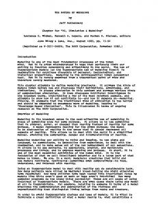
ing vortex filaments that are released at the tip of the blade, and which are discretized in time (ψ) and space (ζ). A schematic of the wake discretization is shown in Figure 1. The distortions of the wake geometry due to maneuvers are taken into account in both models, without a priori assumptions on the geometry. The behavior of the vortex filaments is described by a convection equation of the form dr (ψ, ζ) = V (r (ψ, ζ)) dt
(2)
NS X � � Ibi,j + IN W i,j Γj = V∞i (θi − φF W i )
which for a rotor can be written as 1 ∂r (ψ, ζ) ∂r (ψ, ζ) + = V (r (ψ, ζ)) ∂ψ ∂ζ Ω
lation between consecutive segments is trailed behind the blade at segment endpoints, with a vortex strength equal to the difference between the two segments bound vortex strengths. These trailed vortices comprise the near wake, which is assumed planar and with a fixed angular length. The tip vortex that constitutes the free wake extends beyond the near wake with a strength equal to the maximum bound circulation along the blade. The governing equation for the Weissinger-L method is written as
(3)
where r(ψ, ζ) defines the position of a point on the vortex filament and V(r(ψ, ζ)) is the local velocity at that point. The wake geometry is discretized in two domains, ψ and ζ. The first represents the time component and is obtained by dividing the rotor azimuth domain into a number of angular steps of size ∆ψ. The second represents the age of the vortex filament, which is discretized into a number of straight line vortex segments of size ∆ζ. The right hand side (RHS) of Eq. (3) is determined by the addition of the freestream velocity, the velocities induced by all the other vortex filaments and the blades, plus other external velocities such as those due to maneuvering. The induced velocity is the most complicated and expensive term to compute. Biot-Savart law is used to calculate the induced contribution of each vortex segment at any point in the wake. The discretization of the left hand side (LHS) of Eq. (3), the integration scheme and how it is implemented depends upon the type of free wake model used. The bound circulation is obtained using a Weissinger-L lifting surface model. In this model, the blade is discretized into NS segments. At each segment, a control point is located at 3/4 of the chord, while the bound circulation is placed at the quarter-chord location, and is assumed constant along the segment. The difference in circu-
(4)
j=1
with i going from 1 to NS . Ibi,j and IN W i,j are the bound and near wake influence coefficient matrices, respectively. The stream velocities at the control point, V∞ , are provided by the flight dynamics model and include the velocity due to the translation and rotation of the helicopter, the velocity due to the blade motion and flexibility and the induced velocities. Relaxation Free Wake The Bagai-Leishman model discretizes the LHS of the governing equation in both the ψ and ζ domains. For both, it uses a five-point central difference approximation, which is second order accurate in both ψ and ζ. The stencil for this approximation is given by ∂r(ψ + ∆ψ/2, ζ + ∆ζ/2) = ∂ψ [r(ψ + ∆ψ, ζ + ∆ζ) − r(ψ, ζ + ∆ζ)] + 2∆ψ + [r(ψ + ∆ψ, ζ) − r(ψ, ζ)] (5) 2∆ψ
Dψ ≈
The spatial derivative Dζ is defined in the same manner. The integration method is a pseudo-implicit predictor-corrector (PIPC) scheme, with some form of numerical relaxation. Relaxation methods enforce periodicity, with the consequent limitation of being applicable only for steady-state flight condi-
tions. However, they are usually free of the numerical problems that affect time marching methods and converge rapidly. The relaxation free wake model has already been coupled with the rotor and fuselage dynamic models, and used for the prediction of trim and response to pilot inputs (Ref. [Ref. 2]). One of the key results of the study was that it was possible to predict accurately the off-axis response to pilot inputs, for small amplitude maneuvers, but it required both a flexible blade model not limited to one elastic flap mode and a free wake model capable of modeling the wake distortions due to the maneuver. If one of these two ingredients was omitted, the predictions were qualitatively incorrect. On the other hand, the prediction of the on-axis response was considerably less demanding. Time Marching Wake As for the relaxation model, a five-point central difference scheme, described in Eq. (5) is used for the spatial derivative, Dζ . For the time derivative in the ψ direction, however, a predictor-corrector with second order backward (PC2B) scheme is used, which is also second order accurate, and is given by
The trim procedure used in this study is based on that described in [Ref. 12] and [Ref. 13], which use a dynamic inflow model to obtain the induced velocities, and which was expanded to include a relaxation free wake model in [Ref. 14]. The flight condition is determined by the velocity V , the flight path angle γ and the rate of turn ˙ which define a coordinated steady helical turn. ψ, Straight and level flight becomes then a particular case in which both the flight path angle and the rate of turn are zero. The trim equations are a system of non-linear algebraic equations, namely • Three force equilibrium equations. • Three moment equilibrium equations. • Three kinematic equations relating the rate of turn to the body angular velocities. • A turn coordination equation. • An expression for the flight path angle. • Four equations to determine the inflow coefficients for the main and tail rotors. • The rotor equations, the number of which depends on the quantity of retained modes used in modal coordinate transformation and the number of harmonics used for each mode.
∂r(ψ + ∆ψ/2, ζ) = ∂ψ 3r(ψ + ∆ψ, ζ) − r(ψ, ζ) − 3r(ψ − ∆ψ, ζ) 4∆ψ −r(ψ − 2∆ψ, ζ) (6) 4∆ψ
Dψ ≈
Although this method is potentially subject to numerical instabilities, it is not restricted by the flight condition. Because time marching methods do not need to enforce any type of boundary condition, they are suitable for transient conditions in which periodicity can not be enforced, and therefore relaxation methods can not be used rigorously. Such flight conditions include maneuvering flight or operations in descending flight in vortex-ring state. The baseline trim procedure
The vector of trim unknowns is
X
=
[θ0 θ1c θ1s θ0t αF βF θF φF λ0 λ1c λ1s λt . . . 1 1 1 1 1 1 . . . q01 q1c q1s q2c q2s . . . qN qN ... hc hs Nm Nm Nm Nm Nm Nm > . . . q0Nm q1c q1s q2c q2s . . . qN qNh s ] (7) hc
where θ0 , θ1c , θ1s and θ0t are the collective, cyclic and tail pitch, respectively, αF , βF , θF and φF are angle of attack, sideslip, pitch angle and bank angle of the fuselage, λ0 , λ1c , λ1s and λt are the dynamic inflow coefficients for the main and tail rotor, and the qxk terms are the constant and harmonic coefficients of the k th blade mode.
A nonlinear algebraic equation solver is used to obtain a solution to the system of rotor-fuselage equations. This solver uses a modified Powell hybrid method ([Ref. 15],[Ref. 16]). It builds a Jacobian matrix by a forward difference approach, and then finds a better approximation to the solution by iterating the trim vector. Coupling of free wakes and rotor-fuselage model For a successful coupling with the free wakes, the flight dynamics model must provide the following input: 1. The distribution of the velocities at all points in the blade around the azimuth, not including the inflow, in all three directions, Vx (ψ, r), Vy (ψ, r), Vz (ψ, r). 2. The equivalent rigid blade flapping angles, β(ψ). 3. The hub linear u, v, w, p, q.
and
angular
velocities,
The free wake model returns the inflow distribution for that particular flight condition, λ(ψ, r). For the flight dynamics model and either free wake model to interact correctly, several other details need to be taken into account, such as proper transformation between the coordinate systems used by both models [Ref. 1], as well as interpolation between the different radial and azimuthal points at which each model computes their values. Moreover, the free wake models, which are designed for an isolated rotor and contain their own flapping and trim calculations, must be modified so that the values passed from the flight dynamics model are not overwritten. Trimming with free wake: the two-step trim procedure The overall schematic of the coupling of the timeaccurate wake with the rotor-fuselage model is described in Figure 2. There are two basic phases, namely, trim and transient analysis. As far as the transient analysis is concerned, the coupling
is “loose”. The rotor-fuselage equations are integrated for a specific time interval (e.g., 10o of azimuth angle) for constant inflow. The free wake is then advanced over the same time interval, with the time history of the rotor-fuselage states just calculated. The inflow at the end of the time interval is then held constant while the rotor-fuselage equations are integrated for another time interval, then the wake is recalculated, and so on [Ref. 17]. The trim phase, which is the focus of this paper, is more complex. For a shaft-fixed condition, it would be typically possible to integrate the timeaccurate wake equations until a steady-state solution is reached. Through a simple Newton-Raphson scheme, it would also be possible to adjust the controls until some form of trim (e.g., desired CT and zero flapping) is obtained. This simple procedure is impractical or impossible to apply when the wake is incorporated in a complete flight dynamic model. In fact, the numerical transient encountered before the steady-state solution is reached acts as a forcing function for the complete helicopter model. If the configuration is unstable (e.g., it has an unstable phugoid) a steady-state solution will never be reached. If the configuration is lowly damped, a steady-state solution might be reached, but with a very slow convergence. Damping could be increased through the use of a fictitious flight control system, but the procedure then becomes ad hoc and not guaranteed to work in every case, especially in the case of steady turns. In theory, the relaxation free wake model could be used to compute the trim solution. Then, because the underlying mathematical model is essentially the same as that of the time-accurate wake, the geometry obtained using relaxation would be the same as that of the time-accurate wake. If a subsequent time-marching simulation was desired, this geometry would provide the correct initial conditions. In practice, however, the relaxation solution is close but not identical to a steady-state solution for the time-accurate wake, mostly because of the different numerical schemes used for the solution. As a consequence, in switching from the for-
mer to the latter numerical transients still appear, with the same problems previously mentioned. The solution involves an intermediate ”convergence” phase between the trim calculation with the relaxation wake and a subsequent time-marching simulation using the time-accurate wake. With the rotor-fuselage states and controls fixed at their trim values, the time-marching free wake is run until all the numerical transients disappear. Then the rotorfuselage states and controls are released, and the time-marching simulation can start with the correct wake geometry and no numerical transients. To include the relaxation free wake model in the trim calculation, several modifications need to be done to the baseline trim procedure described above. To start, the main rotor inflow coefficients and the dynamic inflow equations corresponding to the main rotor are removed. The induced velocities are instead provided by the free wake model, which is solved separately at every step of the trim iteration. While greatly based on the process described in [Ref. 14], there are some differences in the current implementation, and thus a brief description of the process is presented here. The method is described in Figure 3. Starting from a guess solution, the algebraic equation solver iterates to find a solution in the same way as in the baseline trim procedure. However, at each iteration, the inflow needs to be determined to calculate the aerodynamic loads with the free wake model. As pointed in [Ref. 14], the interdependence of the inflow and the circulation requires that a double loop is used to solve iteratively for the solution of the free wake. For each vector of trim unknowns, [Ref. 14] calculated the flap angles and the circulation, and used these to determine the induced velocities. The newly calculated inflow was then used to compute an updated circulation, which in turn was used to obtain a new converged free wake and inflow, and the process was repeated until the inflow between iterations converged. In the present study, the introduction of a new circulation methodology allows for an inverted inflow-circulation loop. Rather than using a two-
dimensional sectional lift theory to calculate the circulation distribution, the present study takes advantage of the Weissinger-L method included with the free wake model, allowing for the inclusion of three-dimensional effects such as tip loss. Using the Weissinger-L method offers the possibility of updating the bound vortex strengths for each step of the free wake loop. The process is demonstrated in Figure 3. For each guess of the solution, the velocities seen by the blade due to the combination of translation, rotation, blade motion and blade flexibility are calculated, as well as the equivalent flapping angles. These, together with the body rates and velocities, are passed to the free wake model, which adds the inflow to the blade velocities to calculate the circulation distribution. With this circulation, the free wake iteration starts, determines the geometry and the corresponding induced velocities, and then updates the circulation distribution for these. The process is then repeated until the inflow converges, or the maximum number of set iterations is reached. After trimming the helicopter with the relaxation free wake model, and before computing the transient response with a time-marching free wake, the intermediate convergence phase needs to be introduced. The details of the process are described in Figure 4. Starting from the trim solution, obtained with a relaxation free wake, and fixing the states and controls at their trim values, the flap angles and the blade velocities are calculated and passed to the time-marching free wake model. With these, the circulation distribution is calculated with the Weissinger-L method and the time-marching process is started. At every step of the time-marching solution, the circulation is updated with the most recent inflow. The process is repeated until convergence is reached, or for a number of revolutions long enough such that all the numerical transients have disappeared. After that, the integration of the equations of motion with the time-accurate free wake can start, with an initial geometry free of the numerical transients caused by the two different numerical schemes.
Illustrative Results The results shown in this study have been obtained for a helicopter similar to the UH-60, except that the blade is assumed to have a straight tip, and the airfoil is constant along the blade, at 16,000 lbs and an altitude of 5250 ft, with a bare airframe configuration (flight control system off). To reduce computational cost, only two blade modes are retained in the modal coordinate transformation, the rigid flap and lag modes. The blade is model with four finite elements, and 32 points along the blade are considered. The free wake has been modeled with 4 free turns downstream of the rotor. A 10o discretization is used for both the time and space derivatives. The relaxation free wake was used to trim the helicopter for a range of speeds from hover to 120 kts. The present paper focuses on the low and transition speed range, which is the most critical and difficult to obtain accurately. Three cases for straight and level flight are analyzed in detail: hover (equivalent to 1 kt), 20 kts and 40 kts. The main rotor power required is compared to the results obtained with flight test data and with dynamic inflow in Figure 5. The results obtained with the relaxation wake compare favorably with those computed with dynamic inflow. Although slightly lower than the fight test data available at lower speeds, these results present a significant improvement over the implementation in [Ref. 1], which greatly overpredicted the power required to hover for the UH-60. After the trim condition has been found with the relaxation free wake, and before one can use this solution to determine the response of the helicopter to some arbitrary pilot input, the time-marching free wake needs to be converged to eliminate the numerical transients that would otherwise interfere with the actual response. The process has been described in the previous section. In particular, the time-marching free wake is allowed to run for a maximum of 200 iterations, corresponding to 50 revolutions, or until convergence is reached. The convergence is determined by the RMS of the in-
flow difference between successive iterations, and for the present study the free wake was considered converged if the RMS went below 10−4 . Figure 6 shows the iteration history of the inflow RMS for the three cases considered. For higher speeds, the time-marching free wake converges before the maximum number of set iterations. In particular, the 40 kt case converges after 66 iterations. At lower speeds, the inflow difference between consecutive time steps does not go very low, due to fact that the vortices remain much closer below the rotor and thus any changes in their positions affect the inflow much more than at higher speeds. At higher speeds, the wake geometry is left behind the rotor quickly and convergence is more frequent. Figure 7 shows the top view of the geometry obtained with the time-marching free wake model after it has been allowed to run for 50 revolutions or until convergence, for the speeds of 1kt, 20 kts and 40 kts. For the near hover case, the geometry maintains a circular pattern seen from the top that corresponds with the expected helical structure of the wake in this flight condition. As the speed increases, the wake begins to trail behind the rotor and to rollup on both the advancing and the retreating sides. The differences between the geometry of the trimmed free wake, determined by the relaxation free wake, and the converged time-marching free wake are shown for 1 filament only in Figure 8, for the same speeds as before. For the 1 kt case, the difference between the geometries obtain with both free wake models are minimal. At 20 kts, these differences start to become more significant, but for the first two revolutions of the filament they are still very close. For the 40 kt case, however, the differences appear to be important and need to be investigated further. The side view of the converged time-marching free wake geometry is shown in Figure 9. The 1 kt case presents a helical structure that only breaks far downstream of the rotor [Ref. 3]. As the speed increases, the wake begins to skew, and the vortices begin to interact as their proximity increases.
Figure 10 shows the comparison between the relaxation trimmed geometries and the time accurate converged geometries, seen from the side and for one filament only. These figures reveal some details not observed from the top. For the 1 kt case, it can be seen that the geometries are significantly different in the far stream of the rotor, although these differences so far from the rotor have no influence on the rotor inflow. The differences at 20 kts start to become significant further up in the wake structure, but still far from the rotor. The differences at 40 kts are are better evaluated from the side view than from the top, and appear to be significant enough to affect the induced velocities. Similarly, the rear view of the time-marching free wake geometries is shown in Figure 11. In hover, the wake geometry appears helical as well from the back. The rollup that characterizes the wake in forward flight becomes visible at 40 kts. The same differences observed from the top and from the side between the relaxation and time marching free wakes are seen as well in the rear view, shown for all three speeds again in Figure 12. Additionally, it can be drawn from this perspective that the bigger differences that appear with speed occur in the advancing and retreating sides, where the rollup occurs. The two free wake models predict a similar location for the vortex filaments at the front and rear of the rotor. While the geometry is important is as much as it determines what the actual inflow distribution will look like, it is the induced velocities that are necessary for the flight dynamics model. Figure 13 shows the inflow distribution over the entire rotor for the three cases being analyzed. At 1kt, the distribution looks almost axially symmetric, although not perfectly axial because of the orientation of the rotor which makes some cyclic pitch necessary even in hover. As the speed increases and the wake starts to move back, the effect is reflected as well in the induced velocities as well. At 20 kts, the inflow increases in the rear half of the the rotor. With higher speeds, an upwash is observed in the front of the rotor. In addition, the region where the rollup starts,
in the rear advancing and rear retreating areas, sees an increase in the inflow due to the proximity of the vortices concentrated there. To determine whether the two-phase trim procedure can be used as the starting point of the integration of the equations of motion with the timemarching free wake, it is important to evaluate the difference in the inflow between the two free wake geometries. If the difference is large, the system might see it as a perturbation and the time histories of the states might contain large errors. The difference between the relaxation and the time-marching induced velocities is shown in Figure 14. For hover and 20 kts, the difference is negligible, given that for the first two to three full revolutions of the vortex filaments both models give very similar predictions. For 40 kts, however, there are two regions in which these differences are significant, and these correspond to the areas affected by the rollup of the vortex filaments in the advancing and retreating side. It is in these areas that the two models seem to present the bigger differences in their prediction of positions of the vortex filaments. Figure 15 shows the distribution of the angle of attack for the three speeds considered. At hover, the angle of attack is axially symmetric and mostly uniform. At 20 kts, the angle of attack increases mostly at the outer front and rear of the rotor, and as the speed increases the angle of attack grows in the retreating side, where the speed seen by the blade is lower. Figure 16 presents the distribution of elemental lift, CL M 2 , over the rotor, for the same three cases. In hover, as for the induced velocities and angle of attack, the elemental lift is quasiaxially symmetric. As the speed increases more lift is produced in the regions of higher angle of attack. In addition to level flight, the model has also be used to study steady turns. Two cases are presented, a turn at 10 deg/sec, at a bank angle of 24.6o and a load factor of 1.1, and another at 15 deg/sec, with a bank angle of 34.5o corresponding to a load factor of 1.2. Figure 17 shows the top, side and rear views of the free wake geometry for one filament, at the
end of trim, with the relaxation model, and after the time-marching convergence, for the turn at 10 deg/sec. The differences in the two geometries seem significant, although a closer look reveals the same differences found at 40 kts, i.e., that the main differences are the the far wake and that the rollup prediction is significantly different with the two different models. The same geometries are shown in Figure 18 for the turn at 15 deg/sec. The same behavior is observed, but at this higher rate of turn the relaxation free wake’s prediction on the advancing and retreating side indicates a much larger rollup than the time marching wake does. Figure 19 shows the induced velocities for the straight flight at 50 kts as well as the two turns. As the rate of turn incrases, the inflow increases as well. Comparing Figures 17 and 18, it can be seen that the vortex filaments stay closer to the rotor for the higher rate of turn, and thus the higher inflow distribution. Figure 20 shows the difference between the inflow obtained with the relaxation free wake and the time-marching free wake for both turns, and the significant differences in the rollup prediction, specially in the 15 deg/sec turn, are reflected in higher errors found in the areas of the rotor close to the rolled up geometry.
The main conclusions obtained from the present study are summarized below: 1. The current implementation of the relaxation free wake model can be used to obtain a trim solution that correlates very well with the results obtained with other inflow methods, such as dynamic inflow. 2. For hover and low speed, the geometry and inflow obtained with the relaxation and timemarching free wakes are very similar. The main differences in the geometry appear in the far wake, and therefore have little effect on the inflow. The two-phase trim process would therefore be a good starting point for a transient response. 3. At the higher transition speeds, the differences between the geometries obtained by both free wake models move closer to the rotor, and therefore are reflected by higher changes in the inflow. These changes are mostly in the advancing and retreating side, where both models show significantly different predictions for the location of the vortex filaments. The effect of this differences in a possible transient response needs to be investigated further.
Summary and Conclusion A flight dynamics simulation was coupled with a relaxation free wake model and a time marching free wake model with the ultimate objective of determining the transient response of a helicopter using a time accurate free wake. The need to have an accurate starting solution to obtain the transient response led to the development of a two-phase trim process, in which the first the trim solution is found using a relaxation free wake model, and then the time-marching free wake is converged until the geometry is free of numerical transients. The resulting model was used to investigate the differences between inflow and geometries of the trim solution with the relaxation wake and the converged timeaccurate wake.
4. The method was also used for steady turns. The two cases considered, performed at 50 kts and 10 and 15 deg/sec, present the same problems as the straight flight in the transition speed regime, with additional differences in the rollup prediction as the rate of turn increases. Acknowledgments This research was supported by the National Rotorcraft Technology Center under the Rotorcraft Center of Excellence Program. The authors would like to thank Dr. M. Bhagwat, Dr. J. G. Leishman, and Mr. S. Ananthan for providing a copy of the maneuvering free wake code and for many useful discussions.
References 1
Theodore, C. R., Helicopter Flight Dynamic Simulation with Refined Aerodynamic Modeling PhD thesis, University of Maryland, 2000.
9
Houson, S. S., and Brown, R. E., “RotorWake Modeling for Simulation of Helicopter Flight Mechanics in Autorotation,” Journal of Aircraft, Vol. 40, No. 5, September-October 2003. 10
2
Theodore, C., and Celi, R., “Helicopter Flight Dynamic Simulation with Refined Aerodynamic and Flexible Blade Modeling,” Journal of Aircraft, Vol. 39, No. 4, July-August 2002, pp. 577–586. 3
Leishman, J. G., Bhagwat, M. J., and Bagai, A., “Free-Vortex Filament Methods for the Analysis of Helicopter Rotor Wakes,” Journal of Aircraft, Vol. 39, No. 5, Sept.-Oct. 2002, pp. 759–775. 4
Bhagwat, M. J., and Leishman, J. G., “Stability, Consistency and Convergence of Time Marching Free-Vortex Rotor Wake Algorithms of Time-Marching Free-Vortex Rotor Wake Algorithms,” Journal of the American Helicopter Society, Vol. 46, No. 1, January 2001, pp. 59–71. 5
Wachspress, D. A., Quackenbush, T. R., and Boschitsch, A. H., “First-Principles Free-Vortex Wake Analysis for Helicopters and Tiltrotors,” Proceedings of the 59th Annual Forum of the American Helicopter Society, Phoenix, AZ, May 2003. 6
Spoldi, S., and Ruckel, P., “High Fidelity Helicopter Simulation using Free Wake, Lifting Line Tail, and Blade Element Tail Rotor Models,” Proceedings of the 59th Annual Forum of the American Helicopter Society, Phoenix, AZ, May 2003. 7
Kothmann, B. D., Lu, Y., DeBrun, E., and Horn, J. F., “Perspectives on Rotorcraft Aerodynamic Modeling for Flight Dynamics Applications,” Proceedings of the AHS Fourth Decennial Specialists’ Conference on Aeromechanics, San Francisco, CA, Jan 2004. 8
Horn, J. F., Bridges, D., Washspress, D. A., and Rani, S. L., “Implementation of a Free-Vortex Wake Model in Real-Time Simulation of Rotorcraft,” Proceedings of the 61st Annual Forum of the American Helicopter Society, June 2005.
Saberi, H., Khoshlahjeh, M., Ormiston, R. A., and Rutkowski, M. J., “Overview of RCAS and Application to Advanced Rotorcraft Problems,” Proceedings of the AHS Fourth Decennial Specialists’ Conference on Aeromechanics, San Francisco, CA, Jan 2004. 11
Peters, D. A., and He, C. J., “Correlation of Measured Induced Velocities with a Finite-State Wake Model,” Journal of the American Helicopter Society, Vol. 36, No. 3, July 1991, pp. 59–70. 12
Celi, R., “Helicopter Rotor Dynamics in Coordinated Turns,” Journal of the American Helicopter Society, Vol. 36, No. 4, Oct. 1991, pp. 39–47. 13
Kim, F. D., Celi, R., and Tischler, M. B., “Forward Flight Trim Calculation and Frequency Response Validation of a High-Order Helicopter Simulation Model,” Journal of Aircraft, Vol. 30, No. 6, Nov.-Dec. 1993, pp. 854–863. 14
Theodore, C. R., and Celi, R., “Prediction of the Off-axis Response to Cyclic Pitch Using a Maneuvering Free Wake Model,” Proceedings of the 25th Annual European Rotorcraft Forum, Rome, Italy, Sept. 1999. 15
More, J. J., Garbow, B. S., and Hillstrom, K. E., User’s Guide for MINPACK-1 Argonne National Laboratory, Report ANL-80-74, Aug. 1980. 16
Powell, M. J. D., A Hybrid Method for Nonlinear Equations. Numerical Methods for Nonlinear Algebraic Equations Gordon and Breach, 1970. 17
Ribera, M., and Celi, R., “Simulation Modeling of Unsteady Maneuvers Using a Time-Accurate Free Wake,” Proceedings of the 60th Annual Forum of the American Helicopter Society, 2004.
START
TRIM WITH RELAXATION WAKE
TRIMMED SOLUTION
CONVERGE INITIAL WAKE GEOMETRY
Start Simulation: t=0
Calculate inflow and geometry with timemarching free wake model
Time-marching wake
Save inflow
∆t Save flap and blade velocities
Integrate Equations of Motion at t
NO
Figure 1: Free wake discretization in the azimuth (ψ) and filament (ζ) directions.
Is simulation complete? YES End Simulation: t=T
END
Figure 2: Time integration procedure for the coupling of a time-accurate wake model to the flight dynamics simulation.
TRIM LOOP Trim Guess Tentative Solution
Algebraic Equation Solver
Distribution of Velocities seen by the blade
Rigid Blade Flapping Angles
Trim Solution
Body Pitch and Roll Rates
Equation Residuals
Aerodynamic Model
Calculate Circulation with Weissinger-L Model
Body Velocities
FREE WAKE GEOMETRY
Trim Equations
Free Wake Inflow Distribution FREE WAKE LOOP
Figure 3: Trim procedure with a relaxation free wake model and the bound circulation calculated with a Weissinger-L method.
2000
TRIMMED STATES & CONTROLS
Flight test Dynamic inflow Relaxation free wake
1800
Main rotor power required (HP)
TRIM WITH RELAXATION FREE WAKE
1600 1400 1200 1000 800 600 0
20
40
Save flap and blade velocities
Calculate Circulation with Weissinger-L Model
80
100
120
140
Velocity (kt)
Figure 5: Main rotor power required from hover to high speed, with dynamic inflow and with a relaxation free wake model.
TIME MARCHING FREE WAKE
100
10-1
Inflow RMS
Free Wake Inflow Distribution
60
10-2
10-3 1kt 20kt 40kt
TRANSIENT RESPONSE WITH TIME MARCHING FREE WAKE Figure 4: Schematic of the free wake convergence phase between trimming with the relaxation free wake and integrating the transient response with the time-marching free wake.
10-4 0
50
100
150
200
Iteration number
Figure 6: Iteration history of the inflow RMS during the convergence phase with the time-marching free wake, with 1kt, 20kt and 40kt, until convergence is reached or for a maximum of 200 iterations (50 revolutions).
y/R
1.5
1.5
1.0
1.0
0.5
0.5
y/R
0.0
0.0
-0.5
-0.5
-1.0
-1.0 After trim After convergence phase
-1.5 -1.5
-1.0
-0.5
0.0
0.5
1.0
-1.5 -1.5
1.5
-1.0
-0.5
0.5
1.0
1.5
x/R
x/R
y/R
0.0
2
2
1
1
y/R
0
0
-1
-1
-2 -1.5
-2 -1.5
After trim After convergence phase -1.0
-0.5
0.0
0.5
1.0
1.5
2.0
2.5
-1.0
-0.5
0.5
1.0
1.5
2.0
2.5
x/R
x/R
y/R
0.0
2
2
1
1
y/R
0
0
-1
-1
After trim After convergence phase -2
-2 -1
0
1
2
3
x/R
Figure 7: Top view of the free wake geometry after the convergence phase with the time-marching wake for 1kt (top), 20 kt (center) and 40 kt (bottom).
-1
0
1
2
3
x/R
Figure 8: Top view of a single filament of the free wake geometry after trimming with the relaxation free wake (solid line) and after the convergence phase with the time-marching wake (dashed line) for 1kt (top), 20 kt (center) and 40 kt (bottom).
0.5
0.5
After trim After convergence phase 0.0
0.0
z/R
z/R
-0.5
-0.5
-1.0
-1.0
-1.5
-1.5 -2
-1
0
1
-2
2
-1
0
z/R
1
2
x/R
x/R
0.5
0.5
0.0
0.0
z/R
-0.5
-0.5
-1.0
-1.0
After trim After convergence phase -1.5 -1.5
-1.0
-0.5
0.0
0.5
1.0
1.5
2.0
-1.5 -1.5
2.5
-1.0
-0.5
0.5
1.0
1.5
2.0
2.5
x/R
x/R
z/R
0.0
0.5
0.5
0.0
0.0
z/R
-0.5
-1.0
-0.5
-1.0 After trim After convergence phase -1.5
-1.5 -1
0
1
2
3
x/R
Figure 9: Side view of the free wake geometry after the convergence phase with the time-marching wake for 1kt (top), 20 kt (center) and 40 kt (bottom).
-1
0
1
2
3
x/R
Figure 10: Side view of a single filament of the free wake geometry after trimming with the relaxation free wake (solid line) and after the convergence phase with the time-marching wake (dashed line) for 1kt (top), 20 kt (center) and 40 kt (bottom).
0.5
0.5
After trim After convergence phase
0.0
0.0
z/R
z/R
-0.5
-1.0
-1.0
-1.5 -1.5
-0.5
-1.0
-0.5
0.0
0.5
1.0
-1.5 -1.5
1.5
-1.0
-0.5
0.5
1.0
1.5
0.5
1.0
1.5
0.5
1.0
1.5
y/R
y/R
z/R
0.0
0.5
0.5
0.0
0.0
z/R
-0.5
-0.5
-1.0
-1.0
After trim After convergence phase -1.5 -1.5
-1.0
-0.5
0.0
0.5
1.0
-1.5 -1.5
1.5
-1.0
-0.5
y/R
y/R
z/R
0.0
0.5
0.5
0.0
0.0
z/R
-0.5
-0.5
-1.0
-1.0
After trim After convergence phase -1.5 -1.5
-1.0
-0.5
0.0
0.5
1.0
1.5
y/R
Figure 11: Rear view of the free wake geometry after the convergence phase with the time-marching wake for 1kt (top), 20 kt (center) and 40 kt (bottom).
-1.5 -1.5
-1.0
-0.5
0.0 y/R
Figure 12: Rear view of a single filament of the free wake geometry after trimming with the relaxation free wake (solid line) and after the convergence phase with the time-marching wake (dashed line) for 1kt (top), 20 kt (center) and 40 kt (bottom).
90
90
0.16 1
120
1
120 60
0.14
0.8
0.12
0.6 150
30
0.6 150
180
0
0.06
0
0.2
0.08
0.2
0.01
30 0.4
0.1
0.4
0.02
60 0.8
180
0 −0.01
0.04 0.02 210
330
−0.02 210
330
0 −0.03 −0.02
240
240
300
90
270
−0.04
270
90
0.16 1
120
300 −0.04
1
120 60
0.14
0.8
0.12
0.6 150
30
0.6 150
0.4
0
0.06
0
0.2
0.08
180
0.01
30 0.4
0.1
0.2
0.02
60 0.8
180
0 −0.01
0.04 0.02 210
330
−0.02 210
330
0 −0.03 −0.02
240
240
300
90
270
−0.04
270
90
0.16 1
120
300 −0.04
1
120 60
0.12
0.6 150
30
0.6 150
0.4
0
0.06
0
0.2
0.08
180
0.01
30 0.4
0.1
0.2
0.02
60 0.8
0.14
0.8
180
0 −0.01
0.04 0.02 210
330
−0.02 210
330
0 −0.03 −0.02
240
300 270
−0.04
Figure 13: Inflow distribution after the convergence phase with the time-marching wake for 1kt (top), 20 kt (center) and 40 kt (bottom).
240
300 270
−0.04
Figure 14: Inflow error between the trim calculation with the relaxation free wake and after the convergence phase with the time-marching wake for 1kt (top), 20 kt (center) and 40 kt (bottom).
90
15 1
120
90
60
0.2
60 0.8
10 0.6 150
1
120
0.8
0.6
30
150
0.4
0.15
30 0.4
5
0.2
0.2 0.1
180
0
0
180
0 0.05
−5 210
330
210
330 0
−10 240
300
240
270
90
90
15 1
120
300
1
120
60
0.2
60 0.8
0.8 10 0.6 150
−0.05
270
−15
0.6 150
30
0.15
30 0.4
0.4
5
0.2
0.2
0.1
180
0
0
180
0 0.05
−5 210
210
330
330
0
−10 240
240
300
300
270
−15 90
90
−0.05
270
15 1
120
1
120
0.2
60 0.8
60 0.8 10
0.6 150
0.15
30
0.6
0.4
150
30 0.4
0.2
5
0.2
0.1 180
180
0
0
−5 210
0 0.05
210
330 0
330 −10
240
300 270
240
−0.05
300 270
−15
Figure 15: Angle of attack distribution after the convergence phase with the time-marching wake for 1kt (top), 20 kt (center) and 40 kt (bottom).
Figure 16: Elemental lift distribution after the convergence phase with the time-marching wake for 1kt (top), 20 kt (center) and 40 kt (bottom).
y/R
2
2
1
1
y/R
0
0
-1
-1 After trim After convergence phase
After trim After convergence phase -2
-2 -1
0
1
2
-1
3
0
1
0.5
0.5
0.0
0.0
z/R
-0.5
2
3
-0.5
-1.0
-1.0 After trim After convergence phase
After trim After convergence phase -1.5
-1.5 -1
0
1
2
-1
3
0
1 x/R
x/R
z/R
3
x/R
x/R
z/R
2
0.5
0.5
0.0
0.0
z/R
-0.5
-0.5
-1.0
-1.0 After trim After convergence phase -1.5 -1.5
-1.0
-0.5
0.0
After trim After convergence phase 0.5
1.0
1.5
y/R
Figure 17: Top view (top), side view (center) and rear view (bottom) of a single filament of the free wake geometry after trimming with the relaxation free wake (solid line) and after the convergence phase with the time-marching wake (dashed line) for a 10 deg/sec turn at 50 kts
-1.5 -1.5
-1.0
-0.5
0.0
0.5
1.0
1.5
y/R
Figure 18: Top view (top), side view (center) and rear view (bottom) of a single filament of the free wake geometry after trimming with the relaxation free wake (solid line) and after the convergence phase with the time-marching wake (dashed line) for a 15 deg/sec turn at 50 kts.
90
0.16 1
120
60
0.14
0.8
0.12
0.6 150
30
0.1
0.4
0.08
0.2 180
0
0.06 90
0.04
1
120 0.02 210
330
0
0.6 150
0.01
30 0.4
−0.02 240
0.02
60 0.8
0
0.2
300 −0.04
270
180
0 −0.01
90
0.16 1
120
−0.02 60
0.14
0.8
210
330
0.12
0.6 150
30
−0.03 240
0.1
0.4
300 270
−0.04
0.08
0.2 180
0
0.06 90
0.04
1
120 210
330
0
0.6 150
0.01
30 0.4
−0.02 240
0.02
60 0.8
0.02
0
0.2
300 −0.04
270
180
0 −0.01
90
0.16 1
120
−0.02 60
0.14
0.8 30
0.1
0.4
−0.03 240
300 270
0.08
0.2 180
0
0.02 210
330
−0.04
0.06 0.04
0 −0.02
300 270
330
0.12
0.6 150
240
210
−0.04
Figure 19: Inflow distribution after the convergence phase with the time-marching wake for straight and level flight at 50kt (top), a turn at a rate of 10 deg/sec at 50 kt (center) and a 15 deg/sec at 50 kt (bottom).
Figure 20: Inflow error between the trim calculation with the relaxation free wake and after the convergence phase with the time-marching wake for a 10 deg/sec turn at 50 kts(top) and a 15 deg/sec turn at 50 kt (bottom).