and what into the user's management plan to see how the technology will be used. ... This coating could allow farmers to plant their crops earlier in the ... of planting dates or the number of possible states for each planting date, while ... farm size of 625 acres in a corn and soybean rotation was assumed with 50 percent of the.
SIMULATION MODELING TO PREDICT THE ADOPTION AND ECONOMIC VALUE OF A CROP TECHNOLOGY INNOVATION David W. Archer and Russ W. Gesch USDA-ARS, North Central Soil Conservation Research Laboratory, Morris, MN
ABSTRACT: Simulation modeling is a useful tool for identifying the potential impacts of technology innovations. The use of simulation modeling in this capacity is illustrated for the case of a temperature-sensitive polymer seed coating that has recently been introduced. This information is important both to a company who is trying to market the new technology and to the potential users of the technology. For this analysis, the perspective of a typical farmer as a potential user of the technology is taken. Simulation modeling is used in three ways in the analysis. The effect of random weather events and cropping system are used in the EPIC simulation model to: 1) identify field conditions that determine when the technology can be used and 2) identify crop yields and production costs that quantify what happens when the technology is used. Finally, an economic model is constructed using a decision-tree approach to 3) incorporate the when and what into the user’s management plan to see how the technology will be used. Integrating these three components provides a framework for predicting the extent to which this new technology will be used, the effect of the technology on cropping practices, and the economic value of the technology to crop producers.
INTRODUCTION: When faced with the prospect of adopting a new technology, people must make decisions without the benefit of experience. Simulation modeling can be a useful tool for estimating the potential impacts of technology innovations when direct experience is limited. A temperature-sensitive polymer seed coating has recently been introduced which prevents seed from being exposed to moisture after planting until the soil reaches a pre-set temperature. This coating could allow farmers to plant their crops earlier in the season, protecting the seed and preventing germination until conditions are suitable for crop growth. Before adopting this technology, a farmer needs to know the potential economic impact on his or her farm operation. However, due to uncertain weather conditions, it is difficult to anticipate not only the effect of polymer-coated seed on crop yields, but also determining the extent to which it will even be possible to utilize the technology. Simulation modeling can be used to estimate these effects. In this analysis, we develop a framework for estimating the extent to which polymer-coated seed could be used, the potential effect of the technology on cropping practices, and the economic value of the technology to a crop producer. This approach is illustrated for a representative Minnesota farm.
SIMULATION MODEL: The first step in formulating a simulation framework is to identify how the technology could be used, determining the features that are most important to capture in the simulation. In the case of polymer-coated seed, the technology could potentially allow crops to be planted earlier in the season, so it is important to model the effects of
1
alternative planting dates. Also, with earlier planting, it is possible that longer-season crop varieties could be utilized, so it is important to include crop varieties with differing crop maturities in the analysis. The unique characteristic of temperature-activated polymer seed coating is that it protects seed from germination until the soil reaches a specific temperature. It is important to include this unique characteristic in the analysis as well. It was this aspect that lead to selection of the EPIC simulation model (Sharpley and Williams, 1990) for this analysis. EPIC adjusts planting dates from year to year by checking soil temperature beginning on the specified planting date and initiating planting when the soil temperature reaches a specified minimum. This mimics the behavior of polymer-coated seed that is planted at a specified date, but is not exposed to moisture until the soil reaches a specified temperature and the coating becomes permeable. The seed essentially behaves as if it had just been planted. In order to analyze the potential use of polymer-coated seed under varying weather conditions, 50 years of historical daily weather observations from the University of Minnesota West Central Research and Outreach Center were used to generate distributions of crop yields and field conditions. The EPIC simulations were run for corn and soybean crops with weekly planting dates ranging from April 3 to May 22 for corn (8 weeks) and from April 3 to June 5 for soybeans (10 weeks). Simulations were run for early, normal and late maturity varieties for each crop, and under both conventional tillage (CT) and no-till (NT) systems. Following a modified version of a procedure described by Dillon et al. (1989), soil temperature and moisture values from the EPIC simulations were used to estimate the number of days that would be suitable for fieldwork in each year. The criteria used to identify a nonworking day were: 1) if it
2
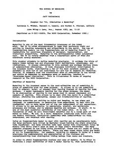
rained 0.15 inches (0.38 cm) or more on a given day, that day was not considered a field day, 2) if soil moisture in the to 3.9 inches (10 cm) was greater than 80 percent of available water capacity for CT, or 90 percent of available water capacity for NT, that day was not considered a field day, and 3) if soil temperature was at or below 32° F (0° C) at any depth, that day was not considered a field day. The next step is to determine how to best utilize the output of the simulations for analyzing the potential use of polymer-coated seed. From the perspective of a farmer making planting decisions during the season, the 50 years of simulation output represent the distribution of possible outcomes at each planting date. The decision process can be illustrated with a decision tree (Figure 1). At the first planting date there are 50 possible yield and field day availability outcomes, or “states of nature”, for a particular crop maturity and tillage. The farmer can decide to plant all or a portion of the farm at this stage, or decide to wait until the next planting period which has another 50 possible states. For the first 2 planting dates there are 50 x 50 = 2,500 states to consider. For the first 3 planting dates there are 503 = 125,000 possible states, and by the end of the tenth planting date there are 5010 possible states to evaluate! Reducing this “curse of dimensionality” problem to a level that can be solved requires reducing either the number of planting dates or the number of possible states for each planting date, while maintaining as much of the underlying information as possible. To reduce the number of planting dates, the yields for weekly planting dates were averaged for each of 4 two-week planting periods for corn and 5 two-week planting periods for soybeans. Expected yields for each of the two-week planting periods are shown in Figure 2. Expected crop yield were lower under NT than under CT. Expected
3
yields decline rapidly for late planting, with late maturity varieties declining more rapidly than early maturity varieties. For the soil type used in this analysis, the late maturity varieties never had the highest yields for a particular planting period. In this case there would be no incentive for a farmer to switch to a late maturity variety, even if it could be planted early. Total available field days were also calculated for these two-week periods. To reduce the number of field day outcomes in each planting period, the distributions of available field days were approximated using two-point Gaussian Quadrature (GQ) estimates. Two-point GQ estimates exactly match the first three sample moments of the field day distributions. Examples of the GQ approximations estimated following the procedure described by Preckel and DeVuyst (1992) are shown in Figure 3. As expected, the simulation showed more available field days in later planting periods than early planting periods. Also, there were more available field days under CT than under NT, particularly in the later planting periods. The distributions of available field days were skewed in opposite directions for early planting periods compared to late planting periods. This highlights the importance using an approximation that captures at least the first three moments of the underlying distribution. The number of available field days in each period may not be independent from the number available in previous periods. To allow for this possibility, the number of available field days in each period was regressed on the number of field days available in previous periods. When these regressions were significant, GQ was used to estimate a two-point distribution for the regression residuals instead of the field days, following Etyang et al. (1998). Field day estimates were then generated from the regression
4
equations and the two-point estimates of the residuals. Also, in some cases the GQ estimates produced negative estimates of the number of available field days. To generate two-point estimates that were feasible, while retaining as much information on the underlying distribution as possible, a simple optimization model was constructed to minimize the absolute deviation from the third moment of the underlying distribution while exactly matching the first two sample moments and requiring the estimated number of field days to be non-negative.
ECONOMIC MODEL AND RESULTS: Reducing the number of planting periods to 5, and approximating the states in each period with two points reduces the farmer’s decision tree to 25 = 32 states of nature. The farmer’s decision was formulated as a Discrete Stochastic Programming (DSP) model (Cocks, 1968). For this analysis, only the risk neutral case was considered, so the farmer’s objective was to choose planting activities to maximize expected net returns. A farm size of 625 acres in a corn and soybean rotation was assumed with 50 percent of the acres in corn and 50 percent in soybeans each year. Costs of production were estimated using the functions in EPIC with equipment cost parameters based on Minnesota Extension Service cost estimates (Lazarus, 2001). No land, overhead, or management costs were included, assuming none of these would change with the availability of polymer-coated seed. Crop prices were fixed at $1.98 per bushel for corn and $5.69 per bushel for soybeans. Planting activities were assumed to be chosen in each period based on the realization of available field days in the current period plus the knowledge of the
5
distributions, but not the realizations of available days in future periods. Labor for field preparation (in CT only) and planting activities was limited by field day availability assuming 12 hours of labor could be used for field work for every available field day. It was assumed that uncoated seed could not be planted prior to period 3 (April 29) for corn and prior to period 4 (May 13) for soybeans. Polymer-coated seed could be planted in any period. It was also assumed that polymer-coated seed purchase decisions were made prior to the first planting period. Polymer-coated seed prices were increased incrementally from $0.00 per acre until no polymer-coated seed was purchased in the model solution. This generated demand curves for polymer-coated seed for corn and soybeans individually. The demand curves are given in Figure 4. At low polymer-coated seed prices, the farmer would purchase enough polymer-coated seed to plant the entire farm. However, on average only a portion of the acres would actually be planted early. The expected portion of the cropland planted in each planting period is shown in Figure 5. Although the farmer would initially be willing to pay a higher price for polymercoated seed under CT than under NT, demand for polymer-coated seed decreased more rapidly under CT. This was due to the more limiting field conditions under NT, which lead to extreme planting delays, and even prevented planting of some soybean acres. Polymer-coated seed can be used to avoid some of these extreme planting delays, preventing large yield losses. For situations where extreme planting delays could be avoided, the farmer would be willing to pay a significantly higher price for polymercoated seed.
6
CONCLUSION: A simulation modeling framework is well-suited to investigate the impacts of new technologies. For this analysis, the potential use and economic value of temperatureactivated polymer seed coating was investigated for a sample farm. The simulation approach allowed the impacts under alternative tillage systems to be considered for a single site. However, the approach is general enough to allow investigation of the technology for other sites with differing soils and/or weather conditions. The EPIC simulation model also could be used to extend the investigation to include potential environmental impacts of the technology including measures of soil erosion, nutrient and pesticide runoff and leaching, and soil carbon storage. The economic model could also be extended to analyze the technology for farms of differing sizes and for farmers with differing risk attitudes providing insights into potential scale and risk management impacts.
7
REFERENCES: Cocks, K. D. 1968. Discrete Stochastic Programming. Mangement Science 15:72-79. Etyang, M. N., P. V. Preckel, J. K. Binkley, and D. H. Doster. 1998. Field Time Constraints for Farm Planning Models. Agricultural Systems 58:25-37. Lazarus, W. 2001. Minnesota Farm Machinery Cost Estimates For 2001. Univ. Minn. Ext. Ser. FO-6696, October 4, 2001. Preckel, P. V., and E. DeVuyst. 1992. Efficient Handling of Probability Information for Decision Analysis under Risk. Am. J. Agric. Econ. 74:655-662. Sharpley, A. N., and J. R. Williams. 1990. EPIC - Erosion/Productivity Impact Calculator: 1. Model Documentation. U.S. Department of Agriculture Technical Bulletin No. 1768. USGPO.
8
Period 1
Period 2 State 1 State 2 z z z
State 1
State n State 1 State 2 z z z
State 2
State n Start z z z
z z z
State 1 State 2 z z z
State n
State n
Figure 1. Multi-period decision tree.
9
CT
NT
160.0
Corn Yield (bu/ac)
150.0 140.0 130.0 120.0 110.0 100.0 0
1
2
3
4
5
6
0
1
2
5
6
0
1
2
3
4
5
6
3
4
5
6
Soybean Yield (bu/ac)
45.0 42.0 39.0 36.0 33.0 30.0 0
1
2
3
4
Planting Period
Planting Period
Maturity
E
N
L
Figure 2. Effect of planting date on expected crop yields.
10
CT March 31 - April 13
CT May 27 - June 9
100%
Frequency
80% 60% 40% 20% 0% 0
2
4
6
8
10
12
14
0
2
4
NT March 31 - April 13
6
8
10
12
10
12
14
NT May 27 - June 9
100%
Frequency
80% 60% 40% 20% 0% 0
2
4
6
8
10
12
14
0
2
Available Field Days
4
6
8
14
Available Field Days
Observations
G-Q Estimate
Figure 3. Observed distributions and Gaussian Quadrature approximations of available field days.
11
NT Corn
Polymer-Coated Seed Price ($/ac)
CT Corn 20.00
20.00
15.00
15.00
10.00
10.00
5.00
5.00
0.00
0.00
0.0
50.0
100.0
150.0
200.0
250.0
300.0
350.0
0.0
50.0
150.0
200.0
250.0
300.0
350.0
250.0
300.0
350.0
NT Soybean
CT Soybean Polymer-Coated Seed Price ($/ac)
100.0
20.00
20.00
15.00
15.00
10.00
10.00
5.00
5.00
0.00
0.00 0.0
50.0
100.0
150.0
200.0
250.0
300.0
350.0
0.0
50.0
100.0
150.0
200.0
Acres Polymer Coated Seed
Acres Polymer Coated Seed
Figure 4. Polymer-coated seed demand curves.
12
Percent of Total Corn Area
CT
NT
100.0%
100.0%
80.0%
80.0%
60.0%
60.0%
40.0%
40.0%
20.0%
20.0%
0.0%
0.0%
March 31 April 14 - April 29 - May 13 - April 13 April 28 May 12 May 26
May 27 June 9
Not Planted
March 31 April 14 - April 29 - April 13 April 28 May 12
May 27 June 9
Not Planted
March 31 April 14 - April 29 - May 13 - May 27 - April 13 April 28 May 12 May 26 June 9
Not Planted
Percent of Total Soybean Area
Planting Date
May 13 May 26
Planting Date
100.0%
100.0%
80.0%
80.0%
60.0%
60.0%
40.0%
40.0%
20.0%
20.0%
0.0%
0.0% March 31 April 14 - April 29 - May 13 - April 13 April 28 May 12 May 26
May 27 June 9
Not Planted
Planting Date
Planting Date
With Polymer-Coated Seed Without Polymer-Coated Seed
Figure 5. Expected portion of cropland planted by planting date.
13