SIMULATION MODELS, GRAPHICAL OUTPUTS, AND STATISTICAL DISCOVERY K. Laurence Weldon Department of Mathematics and Statistics, Simon Fraser University, Burnaby, B.C. Canada Abstract: Both graphics and simulation are tools of increasing use in statistical education and practice. However the parametric traditions of statistics still resist the legitimacy of these technologies. Yet the historical roots of the discipline feature data analysis and probability modeling as principal tools, and graphics and simulation can be seen as the transformation of these roots caused by the computer revolution. With this perspective, much of the theory of statistical inference can be seen as a temporary diversion. This view has implications for both the style and content of statistics courses. The proposal here is that we should be using much more graphics and simulation in our courses, and more focus on data analysis and probability for content. Graphics provide the links between the two areas. It is argued that graphics and simulation allow a broader-based understanding of statistics, something that is both attractive and useful for both students and practitioners. 1. Introduction: The roots of statistics go back to gambling and genetics (probability modeling), and official statistics associated with politics, taxation and vital statistics (descriptive statistics). Applied research in the fields of agriculture and silviculture required designed experiments which led to the development of the theory of inference. The subject has broadened in many directions in recent decades, to include exploratory data analysis, study design, decision theory, Bayesian inference, and resampling techniques. The current diversity of approaches invites an educator to reconsider the scope of the discipline since the historic sequence of topics is not necessarily appropriate for pedagogy. In fact, a re-examination of statistics curricula is helpful in investigating the foundations of the subject. Ironically, there is a sense in which a “back-to-basics” movement in teaching statistics would be an innovation of some merit. More particularly, we argue for a return to a focus on probability modeling and descriptive statistics, the roots of the discipline, for introductory courses. The result would be an innovation because of the impact of computer software on statistical practice and theory.
The impact of computers on statistical practice has been obvious in some ways and subtle in others. The increase in importance of algorithms, graphics, multivariate computations, simulation and resampling methods are fairly clear consequences. More subtle is the decreasing importance of parametric models for inference, optimality of inference methods, the least squares criterion, the common location-scale summaries, and the histogram. Another subtle influence is the increase of trial-and-error methods (or iterative methods) of modeling. Descriptive statistics is the engine behind most modern data analyses: the number one rule for the applied statistician is “look at the data”. Pre-computer constraints limited the scope of data-analytic work with the result that the mathematics of very specialized inference contexts was the focus of the statistician’s attention for several decades. The restrictive traditions of this era have been painfully slow to relax and evolve. In an effort to fill modern needs, some educators in statistics have rejected mathematical statistics and probability modeling in favour of computerized data smoothing and other “informal” methods. While statisticians are aware of the hazards of informal inference, it appears these hazards are no more serious than with the formal pre-computer methods undertaken while the data could not be easily visualized. This view has been convincingly made by Cleveland (1993). His argument for a new paradigm of statistical analysis based on graphics is compelling: the advantages of a graphical approach for inference over classical methods is particularly evident with multivariate data, and in practice, multivariate data is the norm. Descriptive statistical methods have become much more than a first step. Probability modeling is another root of statistical theory that has taken on a new importance in the computer age. Computer simulation has increased the practical utility of probability modeling. Unfortunately, teachers concentrating on data analysis and graphical statistical methods may have reduced the probability content of their courses. However, in the broad view of statistics, observation of a consequence of randomness may be considered data of a kind, and the combination of applied probability modeling and simulation is an effective way of studying such phenomena. The traditional
probability models can be combined to mimic complex systems, and simulation can reveal the properties of these complex systems even when data is absent or incomplete. To understand the potential for this approach, students need to be exposed to it in elementary contexts. Some details of an introductory course in statistics based on probability modeling, see Weldon (1998). A modern training in statistics should have a heavy dose of the use of graphical methods. Graphical methods are important for both data analysis and the study of applied probability models. Until statistical software made graphical methods feasible, both these approaches to the discipline of statistics were held back. In the case of applied probability models, computers not only allowed the simulations themselves, but also the portrayal of findings over the parameter space. In this paper my theme is that graphical methods play an essential role in both statistical education and practice, since they are the key tool in both data analysis and applied probability. 2. The role of graphical methods in learning data analysis In order for statistical education to be useful, the student must learn the intellectual processes needed for statistical practice. This process is not simply an exposure to facts, but exposure to the questions and answers associated with the analysis of data. For example, questions like Have I obtained enough information about the context of this data to analyze it properly? Is this an exploratory study or a confirmatory study? Is there any reason that this data might not be typical of the population of interest? Are there any unusual features to this data, and if so, how will they affect my findings? Should the data be analyzed all at once, or are there natural subsets that require separate analyses? Is there any other data available that I could integrate with this data to improve the analysis?
Can the data be put in a form that makes it more easily assimilated, or more easily communicated? Am I interested in an empirical description of the data, or do I want to compare the data with a explanatory model? Is the objective of my analysis to describe the findings quantitatively or qualitatively? How shall my findings be described for the primary audience of this analysis? These questions arise naturally in discussions of the analysis of particular data sets, as long as the question posed to the student is not too narrow. But they are not questions that can be answered in advance, and the answers taught as dogma. The best way for a student to learn to analyze data is to practice the process. Of course, the guidance and feedback of the instructor are tremendously valuable, but the firsthand contact with real or realistic questions and data is essential to useful learning. In discussions of data analyses, the language of choice is ‘graphics’. The mere mention of correlation, regression, location and scale, smoothing, sampling or normal distribution will have the instructor and the student drawing graphs at each other. So a course in data analysis will require a few icons that students are very familiar with: the density curve, the dot plot, scatter diagram, the contour ellipse for bivariate data, the regression line and conditional densities, and the population-sample schematic. These icons can be combined and duplicated in creative ways that suit the particular needs of a given data analysis. Clearly, graphics is the most important tool for the process of data analysis, and data analysis is the most important skill to teach students who need to analyze data. This claim is increasingly accepted by statistics instructors. In the next section explore the use of graphics to enhance the study of probability models, even when no data is available - this technique is less popular than the use of graphics for data analysis, but may have been underrated so far. 3. The role of graphical methods in simulation
Simulation in statistics is usually used to estimate probabilities or expectations in situations where the analysis is mathematically intractable. However, for all but the most advanced students, most results are unknown and may be considered “intractable” from their point of view. For example, the bias in the usual sample standard deviation may be simply assessed for a particular distribution such as the standard normal. The result for n=5,10,15,20 is -6.0 %, -2.8%, -1.8%, -1.3%. Similarly for the exponential distribution the corresponding result is -14.6%, -7.5%, -5.4% and -4.3%. This simulation experiment can be summarized graphically as:
Percent Bias in the Sample Standard Deviation as a Function of Sample Size 0 Normal Distribution
-5
Exponential Distribution
-10
-15 5
10
15
20
Samplesz
Most students would find the table of data less informative, even though the same information is there. It is doubtful that a formula could do a better job, even if the student knew a formula for this bias. The graph gives a summary of the bias in the sample SD for a wide range of situations, in an efficient and memorable way. The fact that it was produced with minimal knowledge of mathematical or statistical theory is also noteworthy.
Another use of graphics with simulation is to familiarize students with the consequences of random sampling. For example, many students think that a sample of size 30 from a normal distribution will look like a normal distribution. But a few dotplots will show that this is not so; moreover, the grouped-data histogram will not improve things very much for moderate sized samples. The dotplots below are for 5 samples from the N(0,1) distribution.
-----+---------+---------+---------+---------+---------+-2.0
-1.0
0.0
1.0
2.0
3.0
. : . . . : : :..: . ..: ... ..:
..
-----+---------+---------+---------+---------+---------+-z1 . : .. .
: .:. ::. :: . . . : : ..
-----+---------+---------+---------+---------+---------+-z2 .
.
:... . ..:.:.:.. .. .. : . . .
.
-----+---------+---------+---------+---------+---------+-z3 :. . .. . ::...:::: : . . . .. . -----+---------+---------+---------+---------+---------+-z4 . : : :. . . . . . .. :.. . . ::.:.
.
-----+---------+---------+---------+---------+---------+-z5 -2.0
-1.0
0.0
1.0
2.0
The histograms of the same data look like:
3.0
6 5 4 3 2 1 0 -2.0 -1.5 -1.0 -0.5 0.0 0.5 1.0 1.5 2.0 2.5
z1
8 7 6 5 4 3 2 1 0 -2.0 -1.5 -1.0 -0.5 0.0 0.5 1.0 1.5 2.0 2.5
z2
8 7 6 5 4 3 2 1 0 -2.0 -1.5 -1.0 -0.5 0.0 0.5 1.0 1.5 2.0 2.5
z3
10
5
0 -2.0 -1.5 -1.0 -0.5 0.0 0.5 1.0 1.5 2.0 2.5
z4
10
5
0 -2.0 -1.5 -1.0 -0.5 0.0 0.5 1.0 1.5 2.0 2.5
z5
Many basic statistical tools make an assumption of normality. How is one to judge whether a given sample of data is from a normal population? Of course the real question is, does it matter much that I will assume normality in this instance? In any case, if the student learns the futility of trying to recognize normality based on a small sample, this will be a valuable lesson. This example illustrates the use of simulation and graphics to teach about the consequences of randomness in the simplest setting, that of random sampling from a primitive population. However the need for graphics is even more vital in summarizing the outcome of more complex systems. Consider, for example, the following problem: a series of n prizes is to be offered to the contestant in a game show - the contestant can choose any prize as it is offered, but once rejected, a prize cannot be claimed later. The problem is to devise a strategy that will result in the contestant getting a good prize. The quality of a strategy will depend on the distribution of the n prize qualities. The dilemma is that while one collects information about the distribution, many good prizes will be refused. A student can easily study this problem using simulation. The output of the simulation will be a “taken prize” distribution for each prize quality distribution posed. A
plot of these distributions would be a good starting point for selecting a good strategy. To maximize the expected gain may not always suit the contestant’s tolerance for variability. Here is a situation where the student should be motivated to examine the whole distribution of outcomes. A second example of a more complex process is the symmetric random walk. Actually, for this model it is rather easy to produce mathematical results, but the graphical representation makes clear visually things that are very sophisticated psychologically. Most students make the common error of confusing an expected value for the final displacement, 0, with the usual displacement which will be anywhere within 2n1/2 of 0. Consider for example the following typical symmetric random walk portrayals for 500 steps each.
Symmetric random walk 20
10
0
0
100
200
300
step number
400
500
Symmetric random walk 20
10
0
-10 0
100
200
300
400
500
step number
Symmetric random walk 30
20
10
0
-10 0
100
200
300
step number
400
500
Symmetric random walk
30
20
10
0
-10 0
100
200
300
400
500
step number
Symmetric random walk 0
-10
-20
-30
-40 0
100
200
300
400
500
step number
Not only is the increasing variation from 0 evident from the picture, but the apparently systematic trends in either direction are clearly illusions. With this simple example in mind, students will learn to be skeptical of claims made on the mere basis of past observations for trends in the stock market, world climate, earthquakes, etc. It is difficult to make this point convincingly without both simulation and the graphical output of the simulation.
Simulation is used to describe intractable models - the models typically have a few parameters, and the output of the system needs to be described over the parameter space. This description is best done graphically. As an example of this consider again the estimation of the bias in the sample standard deviation as an estimate of the population standard deviation. To cover a large range of distributions, consider the gamma family, with the exponential near one extreme and the normal at the other (the shape parameter of the gamma is 1 for the exponential and infinity for the normal). The sample size, n, is another important parameter for this simulation. One has a graph like the one mentioned earlier but with a different curve for each value of the shape parameter, m. A contour plot, or possibly a 3-D surface plot, could be constructed for the percentage bias as a function of m and n. Now the simulation for this is not really prohibitively time consuming, but it will do as a model for a situation in which the number of the simulated replications must be limited. Suppose we have M levels of m and N levels of n, then we have MN simulated values of the percentage bias and these would not be precisely estimated. We would have to fit a smooth curve through the MN points, much like a regression fit of a Y-surface over a grid of values of X1 and X2. This fitting problem is the same as if we were fitting real data. The use of a parametric model to fit this surface seems illogical - we simply need a smoothed version of the surface indicated by the simulated bias values, a nonparametric smooth being the least subjective. 4. Parametric traditions and graphical communication Statistical tradition is closely tied to parametric inference. The logical simplicity of a focus on a few parameters for data summary has been compelling. But some of this compulsion comes from an inability to produce graphical summaries efficiently. A simple linear regression is often used to describe the predictive relationship between two variables, such as the prediction of weight from height used to assess “ideal” weight. But there is no belief in the fiction of a linear relationship here - it is merely a simple way to approximate the relationship with a two-parameter summary, one that is easy to communicate. However, a good graphical summary can be based on an empirical nonparametric smooth of the data, with any degree of smoothness desired, and without
the constraint of a simple parametric representation. With graphical relationships easy to generate and communicate electronically, the need for a parametric summary diminishes. One argument against the substitution of graphical smooths for parametric summaries, is that if the parameter values have a scientific meaning, and are not merely chosen for a parsimonious fit, then the numerical values must be estimated, and a graphical presentation is not an adequate summary. For example, if one were collecting data on the relationship between the weight of oranges and their packing density, one would want to build into the relationship the knowledge that the oranges were roughly spherical. To omit the parametric aspects of this relationship would be to omit important information. But the use of statistics to describe the input and output of “black boxes” is far more common than the cases where an explanatory model can be constructed. For example, the application of multiple regression analysis in the social sciences rarely will have any justification for the linearity assumptions that are used. Any model with comparable predictive power would be just as useful. The enthusiasm for neural networks in place of classical regression suggests that in many situations, the ability to predict is important even when the model is wrong. By the same argument, graphical summaries produced by nonparametric smooths have a useful role when the mechanism is too complicated to model constructively. Another argument against the use of nonparametric smooths for data summary is that the apparent relationship conveyed by the graph may be untrue. However, the subjective judgment needed to guard against being misled is required for both parametric and nonparametric summaries - in the case of parametric summaries, the class of models chosen is subjective. For example, in regression problems, not only the error distribution, but the choice of independent variables, the assumption of independence of cases, the degree of interactions included, etc. are all subjective choices, and the inexperienced analyst can be deceived. One of the arguments in favour of the use of simulation for exploring properties of noisy systems is that it is easier to do than the mathematical analysis of the system. This
argument also applies to graphical summaries - they are usually easier to do than parametric summaries. 5. When simulated data is like real data, and data summary is needed. For complex systems, the amount of simulation needed to get error-free estimates may be prohibitive. No matter how “super” computers get, there will always be systems complex enough that the ideal degree of simulation of the system will not be feasible. In these cases, our few runs of the system must suffice to describe its characteristics - the statistical problem will be just as if the data were real data. The computer is the laboratory, and we do the experiments we can afford to do to try to learn about the system, in spite of the apparent randomness of the outcome. As an example of this kind of problem, I refer to a simulation described in Weldon (1995). The catch per day of a fishery is described in terms of what is known about the impact of the random arrival of migratory schools of fish in the area, the effect of bad whether on the fishing effort, the elasticity of the local market for fish, etc. Even though simple models are used for each component of this simulated system, the combined system is quite complex - it is not only time consuming to simulate, but there is a complex question of what output measures to simulate. The two graphs below are two typical simulations of 100 days of this model.
2000
CatchWt
1000
0 0
25
50
75
100
0
25
50
75
100
DayNum
1200
CatchWt
600
0
DayNum
The same model produced both graphs, and these are typical of the variety of simulated outputs. These graphical outputs show that large variations in fishing success can be caused by unexplained (random) forces. One wonders whether this simple point would have been seen in a non-graphic summary. Again, the use of graphics as a summary method for simulated data is not simply a failure to do enough simulations - it is an essential feature in the study of the stochastic system.
6. Creativity in data analysis and probability modeling Whether one is using graphics to analyze data or to study probability models, the creative stimulus of the visualizations cannot be denied. If traditional statistical inference has concentrated on reining in our creative urges so we are not overly enthusiastic about possibly transient effects, modern statistics is letting go of the reins in order to broaden the role of statistics to a more exploratory role. Instead of statistics being the inference police, it is becoming the tool of ‘permissive’ research. While we may not want to go all the way, a journey in this direction is probably a good thing. Conclusion The discipline of statistics has been profoundly changed by the electronic revolution. Both the computation and communication aspects of this revolution have required that the mentors of our discipline reassess what they teach. Significant aspects of this change in attitude are the increase in importance of the graphical presentation of results, the simulation of probability models, and the decreased importance of parametric inference. 1. Cleveland, William S. (1993) Visualizing Data. Hobart Press, P.O. Box 1473, Summit N.J. USA 07902-8473. 2. Weldon, K.L. (1995) The role of probability modeling in statistical inference. Proceedings of the South East Asian Mathematics Society Conference: Mathematical Analysis and Statistics: 37-49. Yogyakarta. Indonesia. July 1995. 3. Weldon, K.L. (1998) Probability for Life: A Data-Free First Course in Probability and Statistics. Submitted to the Journal of Statistical Education. (available from the author
[email protected])