American Institute of Aeronautics and Astronautics, Inc. All rights reserved. ...... Antenna/Shuttle Configuration," American Astronautical Society,. Paper 365, 1985 ...
VOL. 13, NO. 4, JULY-AUGUST 1990
691
J. GUIDANCE
Simulation of Actively Controlled Spacecraft with Flexible Appendages R. R. Ryan* University of Michigan, Ann Arbor, Michigan
Complex interplanetary spacecraft and newly proposed satellites for reconnaissance and strategic defense are being designed with increasingly light and flexible appendages despite ever more demanding requirements for accurate pointing and tracking. The onboard control systems required to satisfy these strict requirements during reasonably quiescent conditions must also act effectively to limit deformation and maintain stability of motion in the face of significant disturbances to flexible appendage motion resulting from spin-up, spin-down, orbital, and deployment maneuvers of various types. This paper incorporates a recently proposed theory for modeling flexible bodies into a framework for studying the effects of beamlike appendage deformation on overall system performance. Illustrative examples involving use of the theory hi practical applications are presented, and relative merits of this model theory vs nonlinear finite-element techniques are discussed.
I. Introduction NEW generation of spacecraft designs involving actively controlled systems with extremely light, flexible appendages has motivated increased research aimed at producing accurate models of such systems for purposes of simulation, structural verification, and control law design. A basic requirement of any such model intended for general simulation purposes is that it must be able to account properly for both large overall motions and concurrent small deformations of bodies, as well as to include accurately the important coupling effects existing between these two types of dynamic behavior. Recently, a new technique1 was proposed for modeling the behavior of flexible beamlike appendages attached to a rigid base body undergoing large overall rotations and translations. The theory was developed by considering the base motion to be prescribed as a function of time; effects of the base motion on the small deformation of an elastic appendage were then studied using the new theory and more conventional ones.2"6 The study uncovered limitations of conventional flexible multibody formalisms applied to structural elements and provided the impetus for further development and implementation of the theory into a framework for analyzing free-flying bodies wherein effects of flexible appendage motion on uncontrolled and actively controlled overall system motion could be investigated. The present paper has a threefold purpose. First, in order to extend the theory to deal with free-flying systems without prescribed base motion, the requisite additional kinematical and dynamical equations governing motion of the base are presented, and techniques for incorporating general external forcing effects; such as gravitational attraction and control system actuation, are discussed. Second, in order to illustrate the effectiveness of the model in analyzing spacecraft, simulation results for a few representative problems will be shown, and the effect of the flexible appendage motion on overall base motion will be highlighted in contrast to the aforemen-
A
Presented as Paper AAS 87-0478 at the AAS/AIAA Astrodynamics Specialist Conference, Kalispell, MT, Aug. 11, 1987; received Nov. 2, 1987; revision received March 14, 1988. Copyright © 1988 by the American Institute of Aeronautics and Astronautics, Inc. All rights reserved. *Professor, Department of Mechanical Engineering and Applied Mechanics; currently, Vice President, Mechanical Dynamics, Ann Arbor, ML
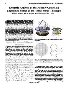
tioned work, which dealt primarily with the effect of base motion on appendage behavior. Last, the enhanced modal approach, on which this work is based, will be compared with nonlinear finite-element formulations aimed at solution of similar problems; relative efficiency, accuracy, and ease of implementation will be discussed. The remainder of this paper is organized as follows. The system to be studied is described in detail in the next section. In Sec. Ill, the theory presented in Ref. 1 is extended to the free-flying case, and supplementary equations of motion are given. Illustrative examples showing general use of the theory and equations in practical applications are included in Sec. IV. The last section concludes with a discourse on the relative advantages and disadvantages of employing enhanced modal techniques rather than nonlinear finite-element procedures to perform simulations of complex deformable spacecraft undergoing general maneuvers. II. System Description The system to be analyzed, shown in Fig. 1, consists of a flexible beam B, fixed at one end to a rigid body A, which is capable of undergoing large three-dimensional translations and rotations in a Newtonian reference frame N. The rigid base is characterized by its mass mA and six independent inertia parameters 7n, /12, /i3, /22> «^23> and /33, which are
Generic Cross-section dB
Fig. 1 Satellite with deformable beamlike appendage.
692
J. GUIDANCE
R. R. RYAN
measure numbers of the central inertia dyadic J of A expressed in terms of a dextral set of mutually perpendicular unit vectors al9 a2, «3, fixed in A, and directed as shown. That is, J = /n
The beam is characterized by a natural length L, material properties E0(x)9 G(x)9 p(x\ and cross-sectional properties A0(x\ I2(x\ I3(x)9 (x.2(x)9 a3(x), K(x)9 Y(x\ e2(x), and e3(x)9 defined as follows. Let x be the distance from a point O, located at the root of B to the plane of an arbitrary cross section of B, when B is undeformed. Then E0(x)9 G(x)9 and p(x) are the beam's modulus of elasticity, shear modulus, and mass per unit length, respectively, each a function of x. The area of the cross section located at a distance x from point O is denoted as A0(x\ and the Saint Venant torsion factor and the warping factor are represented by the symbols K(X) and F(JC), respectively. In order to define the symbols I2(x)9 I3(x)9 a2(x), a3(x), e2(x)9 and e3(x)9 introduce a dextral set of mutually perpendicular unit vectors bl9 b29 b39 fixed in the plane of the cross section located at a distance x from point O and oriented such that b^ is parallel to the centroidal axis of B9 while b2 and b3 are parallel to central principal axes of the cross section. Unit vectors al9 a2, a3 are parallel, respectively, to A!, b29 b3 prior to deformation of B. The symbols I2(x) and I3(x) denote the central principal second moments of area of the generic cross section for unit vectors b2 and b39 respectively, and u.2(x) and a3(;c) are the shear area ratios (also called shear correction factors; see Ref. 7, p. 351) of the section for the b2 and b3 directions. The parameters e2(x) and e3(x) are measure numbers of the b2 and b3 components of the eccentricity vector, which extends from the elastic center of the generic cross section to the centroid. The elastic center, the flexural center, and the center of twist are all assumed to coincide in the present analysis.8 Lastly, the location of the mass center A* of A9 relative to point 0, is specified in terms of three scalar quantites dl9 d29 and d3 representing the al9 a29 a3 measure numbers, respectively, of the position vector extending from O to A*.
III.
Equations of Motion
Reference 1 also treats the system described in Sec. II and contains a detailed discussion of equations of motion applicable when the base motion is prescribed as a function of time. In that regard, a geometric constraint, similar to that proposed by Hughes and Fung,16 was included in the formulation to account properly for the interrelationship of axial and bending deformation in long, thin structural elements, and an algorithm was presented for analyzing general beams attached to moving bases. The treatment of beam deformation using the embedded constraint approach quite naturally leads to dynamical equations that are totally linear in the deformation variables and yet properly account for motion-induced stiffness variations as pointed out by Kaza and Kvaternik.17 The present section is intended to supplement the previous equations with additional equations needed to treat three-dimensional /ree base motion and arbitrary external forcing functions such as might arise from gravitational attraction and active control systems. As before, the interdependencies of orthogonal beam displacements will be properly taken into account in the development of equation terms that represent the coupling effects between flexible appendage motion and large rigidbody base motion. To keep the number of equations to a minimum, terms and expressions developed explicitly in Ref. 1 will, in general, not be redeveloped or rewritten here. Enough detail will be given, however, so that the two papers together provide a complete set of equations and parameter definitions to allow for total understanding as well as construction of algorithms for the
simulation of motions of systems consisting of a rigid base portion and one or more flexible beamlike appendages. In the previous analysis, the motion of the base A was characterized in terms of six scalar quantities coi9 a>29 a>39 vl9 v29 and v39 with col9 co29 a>3 defined as the al9 a29 a3 measure numbers of the inertial angular velocity vector, NwA9 of rigid body A9 and vl9 v29 and v3 defined as the al9 a29 a3 measure numbers of the translational velocity Nv°9 of point O9 on the elastic axis of B at the root, such that t + co2a2 +
(1)
and + t;2a2 + V3a3
(2)
(The elastic axis is the line along which transverse loads must be applied in order to produce bending unaccompanied by torsion of the beam at any section.8 This axis passes through the elastic center E of every section.) The deformation of B9 on the other hand, was described in terms of assumed modal functions ^(x) (y = l,...,6; / = l,...,v) and generalized coordinates qt (i = l,...,v) in such a way that the elastic axis stretch s(x9t)9 the two transverse shear center displacements u2(x9t) and u3(x9t)9 and the three successive rotation angles (see Ref. 1) 9t{x9t) (i = 1,2,3) of a particular cross section, located at a distance x from 0, could be written (3)
Oj{x9t)
J+3,i(x)qM
U = 1,2,3)
(5)
The symbol v in these equations represents the integer number of terms retained in the modal series. With v deformational degrees of freedom and six rigid-body degrees of freedom of A9 it is necessary to form at least v + 6 dynamical first-order differential equations and v + 6 kinematical first-order differential equations in order to determine completely the configuration and state of the system at any instant in time. To facilitate the formation of dynamical equations in the next section, it is beneficial to introduce new quantities, uf (i = l,...,v -f-6), referred to as generalized speeds (Ref. 9, p. 87). These are defined as qt
l,».,v)
(6)
Dynamical Equations The dynamical equations can be written in the form (7)
where Ff. and Ft are the generalized inertia force and generalized active force, respectively, associated with the ith generalized speed uf of the system. Before these generalized forces are given explicitly, it is necessary to form additional kinematic expressions. The inertial velocity of A *, the mass center of A9 can be described in terms of the velocity of point O and the angular velocity of A by using the relationship -Na>Axp°A*
(8)
JULY-AUGUST 1990
SIMULATION OF ACTIVELY CONTROLLED SPACECRAFT
wherep°A* is the position vector from O to A*, expressed in terms of three (not necessarily positive) scalar quantities dl9 d2, and d3, such that (9)
Hence, it follows from Eqs.
(1),
(2),
(8),
and (9) that
N A
v ' = (vt + a>2d} (10)
+ (t>3 +