We provide a substantially more complex mechanism in eqs 3-5 to illustrate ...
Mathematica is instructed to solve the equations by hitting the key combination.
Numerical Integration – Simulation of Chemical Kinetics Using Mathematica 6.0 Mathematica 6.0 Student Edition is licensed through Cornell University and is available at http://www.cusoftware.cornell.edu/cusoftware/purchase/mathematica.cfm
1. Introduction: The Problem Differential equations derived from chemical kinetics must often be solved numerically. The following manual is a detailed guide on how to use Mathematica 6.0 to (1) numerically integrate sets of differential forms of rate laws, and (2) plot the solution as time-dependent concentrations. Given the relatively simple transformations represented in Scheme 1, how can we use numerical integration to solve for the concentrations of A, B, and C for all combinations of rate constants k1, k-1, and k2? A non-limiting case in which the concentration of B builds up to a limited extent is illustrative. Scheme 1
1
2. Differential Forms of the Rate Laws k1 A
B
(1)
C
(2)
k-1 B
k2
We begin by writing the differential equations associated with each chemical species (A, B, and C) in eqs 1 and 2 as follows: d[A]/dt = -k1[A] + k-1[B] d[B]/dt = k1[A] - k-1[B] - k2[B] d[C]/dt = k2[B] We provide a substantially more complex mechanism in eqs 3-5 to illustrate that close attention must be devoted to the stoichiometric coefficients as they translate into prefactorial and exponential terms in the differential equations. k1 B + A2
k-1
A2·B
(3)
k2 A2·B
B + A2
k-2 k3
A·B + 0.5A2
(4)
C + 0.5A2
(5)
This mechanism translates into the following differential equations: d[A2]/dt = -k1[A2][B] + k-1[A2B] + 0.5k2[A2B] - 0.5k-2[AB][A2]0.5 - 0.5k3[A2][B] d[B]/dt = -k1[A2][B] + k-1[A2B] - k3[A2][B] d[AB]/dt = k2[A2B] - k-2[AB][A2]0.5 d[A2B]/dt = k1[A2][B] - k-1[A2B] - k2[A2B] + k-2[AB][A2]0.5
2
3. Numerical Integration in Mathematica We illustrate numerical integration in Mathematica with the example in scheme 1. The differential equations are repeated below with a slight change in syntax. Mathematica does not accept variable names with embedded mathematical symbols (i.e. ‘k-1’, or ‘A*B’). Instead we denote rate constants by a number followed by the letter f or r (forward or reverse). d[A]/dt = -k1f[A] + k1r[B] d[B]/dt = k1f[A] - k1r[B] - k2f[B] d[C]/dt = k2f[B] The input and output illustrated below will be discussed in detail in the following sections.
Part I
Part II
The code is divided into two parts that work in parallel. Part II instructs Part I on how many points to evaluate, over what interval and what solutions it is supposed to find.
3
Part I The input denoted as Part I is repeated below with labels 1-7 referring to the subsequent comments: 1
2
3 4 6
5 7
1. We begin by giving the solution to the numerical integration an arbitrary name such as mechanism1 for recall in part II. The equal sign (=) is normal (as opposed to other cases below). 2. NDSolve prompts the program to numerically integrate the differential equations. The succeeding square bracket ([) is not closed until the very end of part I. The square brackets enclose four sets of curly brackets ({}) explained in the following sections. 3. The first curly bracket ({) encloses the differential equations and initial conditions separated by commas. The time derivative is expressed by an apostrophe followed by [t], indicating that the derivative is taken with respect to time t (e.g. d[A]/dt is written as a’[t]). The double equal sign (==) is constructed from two equal signs and is different from the ordinary equal sign. The two signs visibly merge (tighten up) to form a Mathematica-specific after hitting the space bar. We include spaces between terms only for visual clarity. Each term that is time-dependent (chemical species) must be followed by [t]. Exponential terms follow the [t] (e.g. a[t]^0.5). 4. The initial conditions are treated as linear equations and are part of the set of equations to be solved. Each chemical species must have an initial condition. a[0] == 0.1 sets the concentration of a at t=0 equal to 0.1. We close the equation section of the NDSolve command with a curly bracket (}). 5. The slash (/.) prompts the program to replace all previous rate constants in the equations with the subsequent assigned values. Curly brackets enclose the rate constants separated by commas. The ‘assign’ symbol (->) is formed from a dash followed by a greater-than symbol. Hitting the space bar merges the two symbols (). 6. Curly brackets enclose all chemical species in the mechanism for which a solution is needed.
4
7. Curly brackets specify the time interval (t), starting time (tmin), and ending time (tmax) for which the differential equations shall be solved. We close part I with a square bracket (]) that was originally opened in line 1. Mathematica is instructed to solve the equations by hitting the key combination Shift/Return. Plotting is described in part II. Part II 1 2 3 5 7
4 6 8
1. The output of the Plot command is assigned an arbitrary name (myplot1) for recall. The Plot command is immediately followed by a square bracket, which will be closed at the end of part II. Seven functionally distinct lines of code are organized by numbers 2-8. Lines 2-4 instruct the evaluation of the timedependent variables. Lines 5-8 provide formatting commands. 2. The program is instructed to evaluate variables a, b, and c. If only starting material a is of interest, we would write: {Evaluate[a[t]/.mechanism1]}. The a[t] is followed by /.mechanism1 to indicate that a[t] is evaluated for the set of differential equations defined by mechanism1 in part I. 3. Curly brackets include the time interval over which species a, b and c are to be evaluated (plotted). This time interval should not be larger than the time interval chosen on line 7 in part 1 because the points beyond the interval (>1500 s in this example) will be extrapolated and can be highly spurious. 4. PlotPoints -> 500 tells the program to divide the time interval into 500 points, which would produce points every three seconds in the case provided. Mathematica employs a recursion formula that fills in more points where the curves are most complex (i.e. at inflection points, maximas, etc.). Mathematica also interpolates between the points to arrive at a smooth curve. If the curve is not smooth, increase the number following PlotPoints. If one wishes to display individual points, follow PlotPoints -> 500 with a comma and Mesh->All. 5. PlotRange defines the graphing range. It opens with a curly bracket within which there are two more curly brackets. The first specifies the x axis (time) and the second specifies the y axis (concentration). PlotRange does not interfere with the two time intervals stated earlier. If the time interval is chosen smaller, the program will still evaluate solutions up to 1500 s but only display them to the specified time.
5
6. AxesLabel places labels on the x and y axes, respectively. 7. LabelStyle specifies the color, size, and font of the numbers and labels in the graph. 8. PlotStyle specifies which solutions are to be displayed. In this example, we chose to display all three species a, b, and c. The curly brackets designations for species a, b, and c are listed in the same order as in line 2 of part II (i.e. a, b and c are assigned the colors red, green and blue, respectively).
6
4. Modeling Reaction Orders Reaction orders are easily interpreted for simple kinetic systems, but are often complicated by multiple ground states or parallel pathways. We can model rate order plots and theoretically arrive at a rate order for complex mechanisms using numerical integration. This allows to predict and rationalize rate dependencies when chemical intuition fails. One begins by solving the differential equations as described in section 3 and by computing the slope (initial rate) of the desired time-dependent concentration at various initial concentrations. The initial rates are then plotted against the initial concentration and are fit in Sigmaplot or Scientist to arrive at the rate order. This second step will not be described here. The following code finds the slope (rate) at time=0.2 of species a by computing the first time derivative (D) of the numerical solution of a. These two lines of code are appended to the code presented in section 3. 1
2
3
1. The smooth line seen in the time-dependent concentration plot in section 3 represents an interpolated line drawn through a series of discrete points. The solution is therefore not a continuous function and cannot be differentiated directly. We must first define the solution a[t] as an interpolating function denoted by [t_]. We arbitrarily call it aint. 2. We now take the derivative (D) of the interpolating function (aint) at a specified time. Because we would like to compute the initial rate, we chose an early time point (t=0.2). 3. The solution in this example is 0.0379681. Note that the last two lines are output lines. Computing the initital rates at varying initial concentration of a yields the desired rate order plot.
7
5. Exporting Solutions to Excel The numerical solution that was solved in section 3 can be exported as an Excel file for presentation or imported into fitting programs such as Sigmaplot or Scientist to determine, for instance, whether the computed decay in starting material fits first- or second-order kinetics. The following code exports the numerical solution of a to Excel and is appended to the code presented in section 3. 1 3
2 4
1. We must first collect the time and concentration values separately over a given time range. We define xi as a table containing a time series ranging from i=0 to 1500 in steps of 1. xi now contains 1500+1 time values such that i serves as the index number in the table. 2. Similarly, we define yi as aint that was generated as described in section 4. The Flatten command is necessary to homogenize the tabular format of xi with yi. 3. xi (time) and yi (concentration of a) are grouped together into a table with the name xy. The second curly bracket inside the Table command specifies the index i. In this example, all 1501 points of x and y are exported. 4. Table xy is exported by putting the pathname of the exported file in quotes. The ending xls designates the exporting file as an excel file. The second entry inside the Export command is the name of the table to be exported. The semicolons at the end of every line suppress the output inside the mathematica window. Exported Excel files are overwritten without warning.
8
6. Changing Constants Interactively Slider bars allow you to alter rate constants while watching the curves change in real time. This is done with the Manipulate command as described below using the differential equations described in section 3. 1 2 3 4 5 6 7 8 9 10 11 12 13 14 15 16
Lines 3-11 numerically integrate the given differential equations and are identical to the code discussed previously. Note, however, the placement of the Evaluate command and the lack of assigned rate constants. These are controlled by the manipulate command in the last three lines of the code. The Plot command on line 2 plots the solutions. The formatting options of Plot are specified on lines 12-13 followed by a square bracket. Lines 14-16 are specific to the Manipulate command and define the slider bars. Each rate constant is listed in curly brackets separated by commas. The embedded curly brackets contain the declaration of the rate constant, the default value of the rate constant, and a label name that will appear next to the slider. The name must be placed in double apostrophes. The interior curly bracket encloses lower and upper bound values of the sliders.
9
Shift-Return enables the dynamic command, which allows the sliders to be dragged while the curves adjust interactively. By clicking on the ‘+’ sign to the right of the slider, the current value of the variable is displayed and can be changed continously with the play button. The other buttons are intuitive and warrant no further discussion. The Manipulate command is not limited to rate constants. As an example, a slider can change the initial concentration of species a. To do this, we must assign ‘a’ a variable for its initial concentration. We call it a0. Line 8 must correspondingly be changed to a[0] == a0. Next, we add this new variable to the slider control as described above for the case of the rate constants as shown on line 17. 1 2 3 4 5 6 7 8 9 10 11 12 13 14 15 16 17
Happy Computing!
10