time. 25 30 60 60 65 67 70 100 100 103 105 110 controller state S0 S0 S1 S1 S1 S1 S1. S0. S0. S0. S0. S0 command â di. 0. 0 x x. 1. 1. 1 x x x. 0. 0 status â do.
SIMULATION OF COOPERATING ALGORITHMIC STATE MACHINES USING VERILOG HDL M. G. Arnold and J. R. Cowles and R. D. Joslin J. J. Cupal Computer Science Dept. Electrical Engineering Dept. University of Wyoming University of Wyoming Laramie, Wyoming 82071 Laramie, Wyoming 82071 Abstract Algorithmic State Machine (ASM) charts are useful in the top down design of digital systems. We give examples where the easiest way to transcribe cooperating ASMs into Verilog fails to simulate properly. Although introducing ad-hoc delays might overcome the problem in a particular case, we propose an alternative solution that uses the so called “unknown logic value” x to implement a simple handshaking protocol which schedules the simulation of the ASMs correctly in all cases.
Introduction Hardware description languages [3] for digital systems, such as VHDL and Verilog [8, 9], can be used to synthesize hardware [4, 7] from the description or to describe how the hardware should be tested. HDLs are often used to simulate the behavior of the system at the gate level where the designer provides a structural description of the circuit. For example, in Verilog, primitives such as nand are built in, and can be used to construct more complicated devices, such as a set/reset flip flop: nand #10 n1(q, nq, s); nand #10 n2(nq, q, r); The problem with low level simulation is that the designer must decide on particular gates and structures before the simulation can occur. The need to specify particular devices is incompatible with top down design, where the goal is to defer the physical details for as long as possible. To overcome this limitation, Verilog provides the ability to specify the behavior of a system using behavioral statements. However, proper use of behavioral statements for simulation of cooperating state machines is more difficult than is immediately apparent. Complications arise when the designer wishes to mix behavioral and structural descriptions of more than one cooperating state machine. Because more than one process
is involved in a direct mapping of multiple state machines to Verilog code, we will show that the simulation must model a delay in communications between the machines. If this delay is not modeled, Verilog imposes an arbitrary schedule on the order of execution for the processes. Such an arbitrary schedule creates a defacto delay, which in turn causes undesirable effects, similar to the problems of “delta time” encountered by users of VHDL [10]. The idea of back-annotation [5] of higher level simulations with timing information from gate level simulations has been described, but if this extra information were not provided, the simulation would still be correct from an algorithmic viewpoint. In [5], back-annotation simply provides additional timing accuracy for simulating one state machine. We describe a different kind of timing annotation. Rather than being a luxury that increases simulation accuracy, this timing annotation is actually necessary for the simulation to output the correct result from an algorithmic viewpoint. In other words, a simulation of certain kinds of multiple state machines without timing annotation won’t just be unrealistically fast, it will be wrong.
Top Down Simulation In order to understand the problem discussed here, it is important to understand the top down hardware design approach [6] which we are trying to accommodate in Verilog. Digital systems are easier to understand if the system is partitioned into two parts: the controller and the architecture. The controller implements an algorithm, and in Verilog it is natural to use procedural statements (rather than logic equations or a dataflow description) to describe the controller’s behavior. The architecture, on the other hand, is analogous to a data structure. The designer instantiates simpler modules (counters, ALUs, etc.) to form the architecture, much as a software designer gathers together different fields of data to form a more complicated data struc-
ture. This instantiation is structural, like the nand example above, but at a much higher level, since it often involves interconnection with busses, rather than individual wires. The simpler modules (counters, ALUs, etc.) used to construct the architecture are themselves often machines that can be modeled in a similar fashion. Such step wise refinement can be carried out until the desired level of concreteness has been reached. As mentioned above, it is desirable when exploring design alternatives to keep the level of abstraction as high as possible, and therefore the machines that are structurally instantiated inside the architecture should produce usable simulation results, even though they are only modeled behaviorally. The designer should not be forced to describe every gate that will be needed in the actual hardware in order to obtain a reasonably accurate simulation. The kind of state machines that are simulated here are purely synchronous. All sequential devices in the system are connected to only one clock signal. The devices use this single phase clock to trigger activities, such as state transitions, on the rising edge. Such activity is modeled by Verilog code that follows @ (posedge clk). This causes the process that contains this code to be suspended until the next rising edge of the clock. Meanwhile, other processes may be scheduled. In order to model delays, Verilog also provides # to suspend the process for a specified number of time units; wait( e ) to suspend the process until e becomes true; and @( e ) to suspend the process until the specified change occurs. In the manual design techniques of [6], the controller is described by an Algorithmic State Machine (ASM) chart [1]. This notation describes when the controller issues commands to the architecture, and when the controller should make decisions based on the status signals the controller receives back from the architecture. There are two types of controller commands that the ASM can indicate: conditional (dependent on both the state of the controller and also on one or more status signals) and unconditional (dependent on the state of the controller alone). In ASM notation, the conditional commands are described in ovals and the unconditional commands are described in rectangles. These roughly correspond to the classical Mealy and Moore machines (Figure 1). For example, suppose the Moore type ASM of Figure 1b is to control some architecture. Ideally, we would like to translate Figure 1b into Verilog as: always begin @(posedge clk) present_state = 0; command = 0; if (status)
S0
-� ?
? ��PPP � 0� STATUS PP � P�� 1 � ? � COMMAND2 � � ? S1 COMMAND
(1a)
?
S0
-� ?
? ��PPP � 0� STATUS PP � P�� 1 ? S1 COMMAND ? (1b)
Figure 1: ASMs for Mealy (1a) and Moore (1b) machines. begin @(posedge clk) present_state = 1; command = 1; end end but as the next three sections illustrate, the above Verilog code will not simulate what happens in hardware for some cases. Despite this, we advocate this style because it directly transcribes Figure 1b into understandable Verilog. Spatial position within the code is meaningful, just as in the ASM, giving information about previous and next states. We will introduce a simple annotation technique that allows this style of code to simulate properly in Verilog. There are alternative ways [4, 5, 7, 8] to transform ASMs into Verilog (or VHDL) that will simulate properly. For example, one can simulate the combinational logic needed to generate the command and next state (ns) outputs from the status and present state (ps) inputs: function [1:0] state_gen; input ps,status; reg ns, command; begin command = 0; ns = 0; case (ps) 0: if (status) ns = 1; else ns = 0; 1: begin command=1;ns=0;end endcase state_gen={ns,command}; end endfunction Such representations may be very useful in later design stages, but we reject them for the top level design because they have the same drawback that has long been recognized with gotos in software [2]. In this Verilog
code, textual adjacency gives no information about previous and next states, and so it is difficult to perceive the control flow.
Moore Architecture The simplest situation to illustrate the simulation problem with the Verilog style we prefer is when both the architecture and the controller are Moore machines. The command output of the controller (which is input to the architecture) and the status output of the architecture (which is input to the controller) change simultaneously in an ideal hardware realization. For example, the architecture could be a modulo two counter that ignores the command output from the controller: module arch(command,status,clk); input command,clk; output status; reg status; initial status = 0; always @(posedge clk) status = ~ status; endmodule In this case, the controller hardware of Figure 1b is supposed to synchronize itself to this counter, and produce the command output waveform 180 degrees out of phase from the status input. In fact, when this is simulated with Cadence’s Verilog-XL 1.6 or Wellspring Solutions’ VeriWell/PC, the command output is in phase with the status input. The problem here is that an arbitrary order is imposed by the simulator for events that are scheduled to occur at the same simulation time. When one cooperating state machine depends upon another’s outputs, this arbitrary order is unacceptable. To produce a correct simulation, the controller needs to wait, say for one unit of time, before testing the status input. One way to accomplish this is to use #1 before outputting the command appropriate for each state: @(posedge clk) present_state = 0; #1 command = 0; if (status) begin @(posedge clk) present_state = 1; #1 command = 1; end This allows the architecture to make changes at the clock edge before the controller decides the next state. For this specific simulation, any other delay would suffice. Also putting a single delay after the command output, but immediately before the if would overcome this particular problem:
@(posedge clk) present_state = 0; command = 0; #1 if (status) begin @(posedge clk) present_state = 1; command = 1; end This second approach emphasizes where the delay is needed—just before testing the status. The important observation is that there must be a delay to produce a correct simulation. As above Moore examples, we will describe the location of the #1 as before or after the command for the experiments described in the next two sections.
Mealy Architecture Consider what happens when the architecture is just an inverter. It is obvious that an actual hardware implementation would cycle between the two states, each time choosing the true path of the if, because the test only occurs when the command is 0, and so status (the output of the inverter) is 1 long in advance of the next clock edge. Although the net effect of the architecture and controller is just a modulo two counter that does not really need the decision, this is the simplest demostration of a problem encountered using Mealy architectures. With a delayless inverter as the architecture, three simulations were run: Ctrl. delay State Sequence none 0, 0, 1, 0, 0, 1, . . . after 0, 1, 0, 1, . . . before 0, 0, 1, 0, 0, 1, . . . The controllers without delay and with delay before the command output produce the same incorrect simulation. Such simulations would lead one to believe that the machine is a modulo three counter, since it cycles through state 0 twice, and then goes into state 1. Of course, this is an impossibility for a machine that would be realized in hardware with only one flip flop. The controller with the delay after the command output solves this problem, but only on the assumption that the architecture (the inverter in this example) has no delay. From this example, we can see the cause for this kind of simulation problem: The controller’s statement(s) (if in this example) decide what is to be the next state too early, before the simulator has had a chance to communicate the change in the status that results from the change in the command due to the controller entering the present state. This kind of problem occurs when there is combinational logic in the architecture, as would be the case for a Mealy architecture. A gate level realization of such a machine works properly because it exhibits
a hazard in generating the next state. The state gen approach described earlier simulates properly because it accurately models this hazard by re-executing multiple times during one clock cycle. The semantics of behavioral statements, such as if, do not allow re-execution during one clock cycle.
F0
? ��PP � 0� PP di �P � P� 1 ? F1 do = 1
Moore Problems Erroneous simulations are not limited just to systems that include Mealy machines. Suppose the command signal output from the controller of Figure 1b is the D input of a D type flip flop clocked with the same clock as the controller, and the output of this flip flop is the status signal. Although from a design viewpoint, we want to separate the architecture flip flop (which supposedly contains data) from the whatever flip flop implements the controller, from a theoretical standpoint, the architecture and the controller can be viewed as a single Moore machine. This is an impractical viewpoint for any useful architecture, since the number of states increases exponentially with the number of flip flops, but for this trivial example, it will be helpful to consider the behavior of the system as a whole. There are two possible cycles that a hardware implementation of this system should exhibit, depending on the initial state of the data flip flop. If the data flip flop is initially zero, the command signal, and therefore the status signal (which is just the command output delayed by one clock cycle) will always be zero. This means the controller loops in state 0 forever as the data flip flop also stays 0 forever. On the other hand, if the data flip flop is initially 1 when the controller is in state 0 (for brevity we denote this state of the architecture/controller combination as 10), the combined state machine cycles through the states 10, 01, 10... In Verilog, we ought to be able to model either behavior by a suitable initial block that indicates the contents of the data flip flop before the first clock edge. In order to experiment on this in combination with the controller of Figure 1b, we need a model of a D type flip flop, whose ASM is given in Figure 2. Although there are other ways to model this flip flop in Verilog, such as @(posedge clk) do = di; we want to translate the ASM directly. There are two ways to annotate an ASM with a delay that worked in the last example. Either, the delay occurs just before the command output: module arch(di, do, clk); output do; input di, clk; reg do; initial do = 1; always
-� ? do = 0
? ��PP � 1� PP di �P � P� 0 ? Figure 2: ASM for D type flip flop. begin while (di === 1) begin @(posedge clk); #1 do = 1; end while (di !== 1) begin @(posedge clk); #1 do = 0; end end endmodule or the delay occurs after the command output, just in front of the next state decision: ... #1 while (di === 1) begin @(posedge clk) do = 1; #1; end ... Four combinations of delay were tested: Ctrl. delay after before after before
Arch. delay after after before before
Sequence of Arch./Ctrl. States 00, 00, . . . 00, 00, . . . 00, 01, 10, 00, 01, 10, 00, . . . 00, 01, 00, 10, 00, 01, 00, 10, . . .
In this particular example, no combination of the solutions that worked in the earlier examples produces the correct result. In particular, when both delays are before, there are two different next states (01 and 10) from 00, which is, of course, an impossibility. Although it is likely that a designer could come up with ad hoc solutions to these problems by placing ap-
propriate delays at critical places in a design, this is mostly a trial and error process. Assuming the designer notices the problem, the designer iterates in a frustrating, time consuming, bottom up fashion, not to correct an error in his hardware design, but simply to overcome the limitations of the Verilog simulator. Even more alarming, the simulator might produce the desired results (for example, if the goal were a modulo three counter) when in fact the result is due to a flaw in the simulation. This could mislead the designer to think that the simulation is correct even though the “correct” result was only happenstance.
The Solution: x Handshaking What is needed is a general technique that can be applied in the same way to all state machines and architectural components. This technique should be easy to use, so that the designer can concentrate on the top down design process, rather than on obscure simulation details. Most importantly, this technique should produce accurate simulation results under all circumstances, regardless of what kind or how many machines interact. The general solution that we propose involves timing annotation in a simple, consistent way that allows the simulation of each cooperating state machine to handshake to the simulation of other machines. We are not proposing that the synthesized hardware would need any additional handshaking hardware (if any were needed at all). Instead, we are proposing that the Verilog processes that simulate cooperating state machines and combinational logic follow a simple handshaking protocol. This protocol will automatically schedule the Verilog processes to execute in the proper order to simulate what actions would occur in the actual (nonhandshaking) hardware. Each bit of a Verilog reg or wire can be one of four values: 0, 1, z, or x. The first three of these correspond to the logic zero, logic one, and high impedance states that could occur in the actual hardware. Rather than introducing additional handshaking signals for each status or command signal in the system, we propose to use the value x with the status and command signals themselves, to implement the handshaking protocol. Although x is built in to Verilog, x normally occurs only for unknown values, such as un-initialized variables, and fighting outputs that are connected together. Most built in operators of Verilog return x when any operand is other than 1 or 0, thereby preserving the algebraic properties, such as comutativity, of the operators. The built in operators, and structural primitives, such as nand, do not return x when all the inputs alternate simply between 1s and 0s.
Our handshaking protocol, which goes beyond what the built in operations of Verilog do, is this: When a change occurs (even between 1s and 0s) that will effect an output of a module, the output becomes x at that instant, and then a delay occurs. The length of the delay is at the designer’s discretion, however some # or wait must be present to allow the scheduler to reorder the processes. In another module there must be a #0 wait statement that suspends that module until its input (which was made x by the original module) becomes non-x. Consider implementing the inverter from the earlier example using this protocol, assuming the designer wants to back–annotate this with a delay of two: module arch(command,status); input command; output status; reg status; always @(command) begin status = 1’bx; #2 status = ~ command; end endmodule The Moore controller of Figure 1b also uses the same kind of protocol, except the change that causes the command output to become x is the rising edge of the clock: module control(command, status, clk); input status, clk; output command; reg command; wire status; reg present_state; always begin @(posedge clk) enter_new_state(0); #0 wait(status !== 1’bx); if (status) begin @(posedge clk) enter_new_state(1); command = 1; end end task enter_new_state; input this_state; begin present_state = this_state; command = 1’bx; #5 command = 0; end endtask endmodule
Since each state transition will cause a similar handshake to occur, it is convenient to place these operations in a task. Also, for convenience, the command output defaults to zero when leaving the task. This allows the ASM to be translated directly, only entering “command = 1;” where COMMAND was given in the original ASM. This way command can be omitted in states where it was not mentioned in the original ASM. Since the Verilog scheduler will not have an opportunity to take control away from this process until the next @, #, or wait, changing command from 0 to 1 in state 1 will not cause any problems, since it occurs as an atomic operation within the controller process. It was the designer’s choice to back–annotate the state transition time to be five for this particular machine. The protocol will accommodate the choice of different delays, allowing the designer to back–annotate with reasonably accurate timing information. (The previous examples that did not use this protocol required the timing delays be chosen to schedule the Verilog simulator properly, rather than being chosen to back–annotate what would be observed in a gate level simulation.) The key elements in this protocol are the #0 wait statements that suspend the controller task after making a change in the command (but before deciding the next controller state) and the architecture process (scheduled as a result of this #0 wait) that changes the status to x before Verilog tests if the status is non-x. In the case of the right side of Figure 1, suspending the controller task before the next state decision was simply a matter of putting the #0 wait textually before the if. With other control structures, extra care must be taken to ensure that all possible paths leading to the decision have the appropriate #0 wait statement(s). For example, a while has two paths: one upon entry, and a different one each time through the loop. This is illustrated with the D type flip flop of Figure 2 when implemented using our protocol: initial do = 1; always begin #0 wait(di !== 1’bx); while (di === 1) begin @(posedge clk) do = ’bx; #3 do = 1; #0 wait(di !== 1’bx); end #0 wait(di !== 1’bx); while (di !== 1) begin @(posedge clk) do = ’bx;
#7 do = 0; #0 wait(di !== 1’bx); end end Note that the third #0 wait could be omitted because the only path to the second while is out of the first while, and the #0 wait inside the first loop protects both the re–entry test of the first loop, as well as the entry test of the second loop. In this example, the 0 to 1 delay is 3 and the 1 to 0 delay is 7. These delays were chosen to illustrate that whether status becomes non-x earlier or later than the command, the protocol will function properly. Table 1 shows the signals at the time each change occurs, assuming a clock period of 40. Between times 60 and 67, command stabilizes before status, but between time 100 and 105, status stabilizes before command. In both instances, both state machines choose the correct next state.
Mealy Controller Controllers are often Mealy machines, where some commands (that in turn can trigger changes to some status signals) are issued only when certain conditions (involving other status signals) are true. In a hardware realization, a Mealy controller is often faster and has fewer states than the equivalent Moore controller, and so it is desirable to extend our protocol for this case. In our protocol, the unconditional output(s) are treated like the output of the Moore controller given above: enter new state makes the unconditional output(s) x for a period of time, and then the unconditional output(s) are set to their default value(s). Before releasing control to the scheduler, the code in the controller that immediately follows enter new state will leave the default value(s) alone or will change them to whatever value they are supposed to have unconditionally in that state. On the other hand, conditional output(s) are treated differently: enter new state still makes the conditional output(s) x for a period of time, but it does not set them to their default value(s). Instead, there is another task, which we refer to as exit current state that changes all conditional output(s) that are still x to their default values. In order for this protocol to work, exit current state must be used on all possible paths for exiting from any state. Consider the controller of Figure 1a, which has two outputs: command which is unconditional, and command2 which is conditional. always begin @(posedge clk) enter_new_state(0);
time controller state command ↔ di status ↔ do
25 S0 0 1
30 S0 0 1
60 S1 x 1
60 S1 x x
65 S1 1 x
67 S1 1 0
70 S1 1 0
100 S0 x 0
100 S0 x x
103 S0 x 1
105 S0 0 1
110 S0 0 1
Table 1: Simulation using x-protocol for the controller in Figure 1b with the flip-flop in Figure 2. #0 wait(status !== 1’bx); if (status) begin command2 = 1; exit_current_state; @(posedge clk) enter_new_state(1); command = 1; end exit_current_state; end Note that the second exit current state actually exits from both state 0 and state 1 depending on whether the if occurred. In enter new state, command is set to 0, but command2 is left as x: task enter_new_state; input this_state; begin present_state = this_state; command = 1’bx; command2 = 1’bx; #5 command = 0; end endtask task exit_current_state; if (command2 === 1’bx) command2 = 0; endtask Although in this example, there is only one statement in exit current state, in a larger problem, each conditional output would require a similar if. In the architecture, command and status are connected to an inverter, exactly as in the Mealy architecture discussed earlier. This means the state transitions will be the same as the previous example. Suppose that the conditional output, command2 is the D input to a flip flop. After settling, command2 should be the same as status. The flip flop therefore should output status delayed by one cycle. Our protocol correctly models this behavior. With Mealy controllers, care must be taken that all outputs are non-x before the rising edge of the clock. If exit current state had been omitted, the output of the flip flop would incorrectly stay 1 forever. This error results from command2 being x during the entire
clock cycle, therefore #0 wait(di !== 1’bx) never allows the flip flop process to be scheduled.
Applications to VHDL The problems of simulating cooperating state machines described above are not limited to Verilog. VHDL users have encountered similar problems1 . The widely used std_logic_1164 has nine enumerated values, including ’X’ (forcing unknown), and so our handshaking protocol works in VHDL. For example, the inverter described earlier would be: LIBRARY ieee; USE ieee.std_logic_1164.all; ENTITY arch IS PORT(command:IN std_logic; status:OUT std_logic); END arch; ARCHITECTURE arch OF arch IS BEGIN PROCESS (command) BEGIN status