Simulation of Task Graph Systems in Heterogeneous Computing ...

Simulation of Task Graph Systems in Heterogeneous Computing Environments Noe Lopez-Benitez and Ja-Young Hyon Department of Computer Science College of Engineering Texas Tech University Lubbock, Texas 79409-3104 [email protected]

Abstract This paper describes a simulation tool for the analysis of complex jobs described in the form of task graphs. The simulation procedure relies on the PN-based topological representation of the task graph that takes advantage of directly modeling precedence constraints and other characteristics inherent in Generalized Stochastic Petri Nets (GSPN). The GSPN representation is enhanced with enabling functions that govern the sequence of firings of transitions representing execution of tasks. The regulated flow of activity is carried out observing not only precedence constraints but specific allocation heuristics and communication delays. The tool is useful in evaluating different heuristics described by the corresponding implemented algorithm, or using a deterministic timespan given by a Gantt chart.

1. Introduction Task graphs represent general computation jobs which have been decomposed into modules called tasks that are executed according to some precedence constraints. Task graphs are a well known tool to study performance issues of complex jobs. A direct solution technique for seriesparallel task graphs is reported in [1]; an average completion time of the overall job is derived assuming no restrictions exist on the number and architecture of processing units and with no regard to allocation schemes. Execution times of fork-join parallel programs in multiprocessor environments is discussed in [2]. An approach based on multiplication/convolution is applied to Heterogeneous Computing Systems (HCS) at coarse and fine levels of granularity in [3]. Also, in [4] performance prediction of fork-join task graphs is addressed, where the residence times of each task are estimated in terms of service demands and queuing delays; based on these estimations,

the task graph is then systematically reduced. Markov-based solutions of task graph systems have been reported in [5] and [6]; although limited to relatively small task graphs, a Markov-based solution is used for the analysis of scheduling policies in [6]. Since Stochastic Petri Nets (SPN) provide a natural representation of parallelism and synchronization their use spawns applications from individual parallel and concurrent programs to distributed applications and multi-processor systems [7, 8, 9]. SPN’s can be used to directly capture the topological information of a task graph and provide a systematic way for applying factors such as processor heterogeneity, allocation schemes, communication costs, and random execution times. Also, a SPN-based solution can be applied to arbitrary graphs which are acyclic but not necessarily series-parallel [10]. SPN-based tools automatically generate Markov models that represent the execution process of complex task graphs where each state is given by the number of tasks executing in parallel. These models are then solved to compute system performance characteristics such as a distribution of the overall completion time. When the job represented by a task graph is executed on the processing elements of a HCS, estimating the overall completion time becomes an optimization problem involving the mapping of tasks to processors such that completion time is minimized. Mapping tasks to processing units is a hard problem and several heuristics have been proposed in the literature. However, before choosing the most effective heuristic a method must be available for computing an expected completion time and deriving execution distributions for any given task graph, HCS, and allocation heuristic. The methodology reported in [10] to solve complex task graphs using SPN’s is not in itself an optimization technique, but it can be used in conjunction with optimization techniques which attempt to search a space of completion time distributions. However, Markovbased numerical solutions are limited to exponential distributions and often involve a large state space.

Consequently, the solution process may be unstable and subject to stiffness problems rendering inaccurate results. Discrete event simulation can use the framework provided by SPN’s [11] and circumvent the limitations encountered in the solution of Markov-based models. The work reported in this paper uses the SPN-based topological representation of task graph systems just as in [10] but applies discrete-event simulation to obtain execution time distributions and estimates of the Mean Time to Completion (MTTC) of the jobs represented. Thus a common model based on SPN’s is used to drive a discrete event simulation of the overall job. The method can be used to analyze and compare several assignment heuristics given either the algorithm or a Gantt chart of specific assignment cases. To illustrate the use of the tool several assignment heuristics are evaluated and compared. The next section of the paper introduces the notation and parameters used. Basic concepts on Petri nets are introduced in section three and their application to describe task graphs is given in section four. Section five deals with the simulation methodology. A brief discussion on allocation heuristics is given in section six. The insertion of communication delays is discussed in section six. Simulation algorithms are presented in section seven. Lastly, applications of the tool are discussed.

2. Parameters and Notation Throughout the paper the following notation is used to describe the simulation tool and related issues. • a task graph G(T , E) where the vertex set T = {T 1, T 2 , . . . , T k } consists of k tasks which compose some overall job and the edge set E consists of ordered pairs from T which correspond to data or control dependencies. The topology of T is described in detail by the following: − an in-degree vector D = [d 1, d 2 , . . . , d k ] where d i is the number of tasks which must complete before T i may initiate execution. − an out-degree vector H = [h1, h2 , . . . , h k ] where hi is the number of tasks which are spawned after the completion of T i . − a task graph structure TG[i][ j], 1 ≤ i ≤ k, 1 ≤ j ≤ hi where TG[i] is an array specifying the hi tasks which are spawned by the completion of T i ; thus, the ordered pair (T i , TG[i, j])ε E. • a k × k matrix pkt[i, j], 1 ≤ i, j ≤ k where pkt[i, j] is the average number of data packets of standard size that is sent from T i to T j . Alternatively, these can be specified as edge weights for the elements of E. • a priority vector W = [w 1, w 2 , . . . , w k ] which induces a sequential ordering of any ready tasks assigned to the

same processor; these priorities may be taken from the indices of the tasks, e.g. w i = k − i, or they may be randomly or determined according to the assignment heuristic employed. • a set P = {P 1, P 2 , . . . , P n } consisting of n processors composing a heterogeneous suite. • a k × n execution time matrix B[i, j], 1 ≤ i ≤ k, 1 ≤ j ≤ n where bij is the average execution time of T i on P j . • an n × n communication time matrix C[r, s], 1 ≤ r, s ≤ n where each entry c rs is the average communication time to transfer a data packet of standard size from P r to P s . • a k × n static allocation matrix A[i, j], 1 ≤ i ≤ k, 1 ≤ j ≤ n where entry aij = 1 if T i has been allocated to P j , and 0 otherwise.

3. Basic Petri Net Concepts A Petri net (PN) is a directed, weighted, and bipartite graph [12]. PN’s are bipartite in that nodes are of two types, places and transitions, with arcs occurring either from places to transitions or from transitions to places. When an arc is from a place p to a transition t, then p is an input place of t; a place p is an output place of t if an arc proceeds from t to p. Places and transitions are represented pictorially by circles and thin rectangles, respectively. A third component of any PN are tokens which reside in places; pictorially, tokens are represented by dots within the perimeters of places. Tokens are transferred from one place to another by the firing of transitions. When a transition t fires, tokens are removed from all input places of t and placed in the output places of t; thus, enforcing a logical flow of activity throughout the net. A transition can fire if it is enabled, i.e., if all of its input places possess at least one token. An arc may be weighted where the weight specifies the number of tokens which must reside in an input place in order for a transition to be enabled, or the number of tokens placed in an output place by the firing of an enabled transition; if the weight is unspecified then it is assumed to be one. PN’s and their dynamic behavior can be captured in mathematical notation via state vectors. Given a PN with k places, a marking q of the PN is denoted by M q ; a marking is described by a k − vector whose ith component denotes the number of tokens in place pi ; an initial marking of the PN is denoted by M 0 . A particular PN with an underlying graph N is denoted (N , M 0 ). The reachability graph of a PN is a graph G R (M, ∆) where the vertex set M is the set of all possible markings for the PN and the edge set ∆ consists of all possible transition firings transforming one marking into another.

T4 T1 T5 begin

•

•

end

T2 T6 T3 Figure 1. A simple task graph

Stochastic Petri nets are PN’s in which there is an exponentially distributed delay time between the enabling and firing of transitions. The reachability graph of a bounded SPN is isomorphic to a finite Markov chain (MC) [13]; in particular, the markings of the reachability graph comprise the state space of a MC and the transition rate between any two states X i and X j is the sum of all firing delays for transitions transforming M i into M j . Generalized stochastic Petri nets (GSPN) have been proposed [14] in which transitions are of two types: timed transitions which have the exponentially determined firing rates and immediate transitions which have no firing delay and have priority over any timed transition. Enabling functions are marking-dependent functions which can be defined on each transition as a switching mechanism. Transition priorities (timed vs. immediate) and enabling functions are logically equivalent extensions of SPN which endow them with the full computational power of Turing machines [15]. In this paper the notion of GSPN is used.

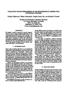
4. GSPN Models of Task Graphs Task graphs are assumed to be series-parallel for several approaches to performance evaluation [16] and optimization [17]; however, this limitation is avoided in the PN-based methodology of this work. Fig. 1 shows a simple task graph which will be used to illustrate the translation of task graphs into GSPNs. The translation of a task graph into a GSPN begins with the association of each task T i with a place/timed transition pair, pi and t i . Fig. 2 shows the GSPN corresponding to the task graph in Fig. 1. Auxiliary places xp0 and xp1 and immediate

transitions it 0 and it 1 are used to enforce initiation and completion conditions, respectively, for the overall job. The presence of at least one token in a place may represent the fulfillment of all preconditions for the initiation of the task. The firing of a timed transition represents the completion of execution of the corresponding task. The delay time of each transition corresponds to the exponentially distributed execution time of the task. A place pi can be associated with the in-degree d i to enforce precedence constraints. Initially, the presence of a token in xp0 enables it 0 ; the firing of it 0 represents the initiation of an execution cycle. The presence of three tokens in xp1 and the firing of it 1 indicates that an execution cycle has been completed. Timed transitions in the GSPN model in Fig. 2 will fire once enabled. Beginning with an initial marking M 0 a sequence of markings can be generated to form a reachability graph. The set of markings generated correspond to the possible execution states of the system, where a system state is defined by the tasks which are executing concurrently. If firing times are exponentially distributed the set of markings generated corresponds to a Markov chain that can be solved using well known tools such as SPNP [18] or SHARPE [1]. Consider some marking M i in which task T 6 should be ready to run. To make this possible, both T 2 and T 3 must have finished execution; this will be indicated by the presence of two tokens in p6 , i.e. x i ( p6 ) = 2. To capture this precedence constraint it suffices to associate each input arc into a timed transition with a weight corresponding to the in-degree of each node in the task graph. Alternatively, the in-degree vector is associated with markingdependent enabling functions.

t4 p4 t1 T4

p1

t5 p5

T1

xp0

xp1

3

T5

t2

it 0

it 1

p2

•

t6 T2

p6 t3

2

T6

p3 T3 Figure 2. GSPN model of the task graph from Fig. 1

5. Simulation Methodology In a SPN model, the firing of transitions represents the occurrence of events, in this case, execution of tasks. To simulate execution of tasks [11], a clock is set for each newly enabled transition to keep track of the execution time until the transition fires. The simulation procedure must also check for precedence constraints, availability of processors, and priority of tasks. When a transition is enabled its firing time is generated as a random variate from a selected distribution. Firing times are recorded by associating clocks to transitions. The PN-based simulation procedure takes place observing the following major steps: 1) Check for newly enabled transitions, 2) Generate firing firing times, and 3) Update clocks.

5.1. Enabling Functions A transition t i is enabled when conditions Qi , V i , and Z i are satisfied. An entry of the enabling vector F = [ f i ], 0 ≤ i ≤ k is evaluated such that if: f i = Qi V i Z i evaluates to one and t i can fire.

Condition Qi checks for precedence constraints, that is, when the number of tokens m i in place pi is equal to the in-degree d i of the vertex representing task T i , its precedence constraints are met, i.e., 1 if m i = d i Qi =  0 otherwise Condition V i checks for allocation and availability of processors. To check for allocation suffices to examine the ith row of matrix A for aij = 1 and then verify if processor j is free. Let a binary vector FREE = [ free j ], 0 ≤ j ≤ n − 1 keep track of which processors are currently free, then V i = aij free j If more than one transition satisfies condition Q and V and their corresponding tasks are allocated to the same processor, only one transition should be enabled (only one task should execute) even though these tasks could execute in parallel. The task with the highest priority is chosen using the priority vector W . Let Rdy be the set of transitions representing parallel tasks allocated to the same processor. That is, the set of transitions that could be enabled from a current marking M, then

1 if w i = max {w j } j ε Rdy Zi =  0 otherwise  Note that these functions could be easily implemented by incorporating additional places and transitions to the model in Fig. 2. For example the presence of a token in a dedicated place can be used to model the availability of a processor and to derive statistical measurements on the usage of that processor [19]. Also additional immediate transitions can be used to model task priorities. It can be argued that additional modeling elements may obscure the representation of a task graph and although they are useful, they become transparent to the user when dealing with large complex models. We find the addition of places to model processing elements and their interconnections useful for the case of analyzing the behavior of systems running several jobs modeled by different task graphs or several instances of the same job in an effort to capture the load of the system, resource contention and usage. In our case the effect of external load is reflected in the execution time of each subtask. The use of enabling functions keeps the model simple and the simulation code relatively simple as well.

iii). Uniform distribution, U(b1ij , b2ij ): x ij = u × (b2ij − b1ij ) + b1ij

5.3. Clock Update A local clock that keeps track of firing times and a global clock is used to record the overall completion time. When a timed transition is enabled a local clock is set to the generated firing time to indicate the remaining time until the transition fires. A global clock is denoted as C and local clocks are represented by a vector LC = [lc i ], 0 ≤ i ≤ k − 1 where lc i is the local clock associated to transition t i . Since local clocks indicate remaining times, they are discarded when they reach 0 time units and the corresponding transitions fire. At the moment a transition fires, the global clock and local clocks are updated. The global clock update is performed by adding the minimum local clock time min_t to the global clock C; min_t is taken from the set of enabled transitions that have not yet fired. The following expressions are used to update all clocks. C = C + min_t lc i = lc i − min_t

5.2. Firing times If a timed transition is enabled, a firing time is generated using a firing transition rate given in terms of the average execution times of each task obtained from matrix B. Random variates are generated from three possible distributions: exponential, normal, and uniform. The values given by matrix B are used according to the distribution function selected. Uniform and normal functions require a second value that must be provided by the user. If B1 denotes the first matrix given as the execution matrix B then B2 denotes a second matrix provided by the user for the case of normal and uniform distributions. For exponential and normal distributions b1ij provides the average execution time. For normal distributions the matrix B2 provides the standard deviation ρ ij . In the case of a uniform distribution, matrix B1 provides the starting point b1ij and matrix B2 provides the ending point b2ij . These values are used to calculate the mean as (b1ij + b2ij )/2. A pseudo-random number u is generated from U(0, 1). A firing time x ij associated to transition t i is generated for each distribution as follows: i). Exponential distribution, exp(b1ij ): x ij = − b1 j × ln(u) ii). Normal distribution, N (b1ij , b22ij ): a=12

x ij = ( Σ u a − 6) × b2ij + b1ij a=1

where min_t = min {lc i }, 0 ≤ i ≤ k − 1. i

Once the last

transition fires, the global clock C indicates the overall completion time.

6. Heuristics Different allocation heuristics can be evaluated by mapping them into the allocation matrix A. To illustrate the use of the simulation methodology discussed in this paper four static allocation heuristics are evaluated and compared. 1. Shortest Estimated Execution Time First (SEETF). In this scheme [20, 21, 22] task T i is selected at random from the task set and assigned to the processor that executes T i faster. The elements of the task allocation matrix from the SEETF algorithm are determined as follows: 1 aij =  0

if bij = min {bij } j

otherwise

2. Minimum Finish Time (MFT). In this allocation scheme [22], task T i is also selected randomly from a topologically sorted task set, i.e. taking into account the precedence constraints between tasks. The selected processor is the one that minimizes the finish time of a task in a deterministic simulated execution, where the finish time of a selected task T i is given by the

minimum sum of its execution time bij and the next time instance in which processor P j becomes a free processor. 1 aij =  0

if min {bij + time until P j is free} j

otherwise

Note that all tasks are selected randomly but restricted to those tasks whose predecessors have already been allocated. 3. Largest Task First (LTF) [22]. The selection of tasks is based on service demands. The task with the largest service demand is selected first, or alternatively the task with the largest execution time is selected first. Thus: 1 aij =  0

if bij = max {bij } i

otherwise

A processor P j is selected randomly. 4. Most Data Task First (MDTF) This scheme selects the task that generates most data. The data generated by a task T i is determined in terms of the number of data packets going out, that is: pkt i =

k

pkt ij Σ j=1

Thus, the construction of the allocation matrix proceeds as follows: 1 aij =  0

if pkt ij = max { pkt i } i

otherwise

and in this case also the processor P j is selected randomly.

7. Communication Delays As in [10], two approaches are presented based on two types of interconnection networks: (a) a high-performance network characterized by high-connectivity and parallel communications and (b) a bus-oriented network with lowconnectivity. In both cases, output data is assumed to be accumulated in a buffer during task execution and transmitted after task completion.

7.1. Modeling High-performance Communication Networks High-performance communication networks can be characterized as expensive systems in which inter-node communication takes place on dedicated, point-to-point links. Data intended for each successor is written to a separate buffer. Furthermore, each processor may be coupled with a front-end communication processor which

enables parallel communication. In terms of a task graph, once a given task completes, successor tasks experience an initiation delay equal to the data transfer time for all intended packets; ideally, any successor task allocated to the same processor as the parent task should be able to begin execution immediately after the completion of the parent task. The properties of such a high-performance network can be modeled in a GSPN by inserting additional place/timed-transitions to represent each individual communication; augmentation of the task graph with communication nodes has been proposed for CTMC-based analysis [23] and at the SPN level [24]. Each timed-transition inserted is associated with an exponentially distributed delay whose parameter is the average communication time between the host processors. Thus, given a completed task T i allocated to processor P r and a successor task T j allocated to P s , the average communication rate assigned to the transition modeling the transfer of data is given by: δ ij =

1 c rs pkt ij

Fig. 5a illustrates a segment of some task graph in which Task A spawns tasks B, C, and D. Suppose the four tasks are allocated to three processors such that A and C are allocated to one processor, and B and D are allocated to the other two processors, then the resulting GSPN for Case 1 would be as shown in Fig. 5b. Note the insertion of place/transition pairs between A and B and A and D to represent the individual In terms of simulation, communication delays are determined from a distribution function using the average delay δ ij and associating a local time to communication tasks.

7.2. Modeling Bus-Oriented Networks In interconnection networks characterized by low-connectivity, groups of processors may have to share common communication links, as is the case with a bus-oriented architecture. Also, in lower cost systems processors may be forced to expend computation cycles on communication processing. If, additionally, output data packets for successor tasks are queued up in a single buffer in some random ordering and transmitted on a FIFO basis, then it is highly unlikely that a successor task will receive all of its packets before any other successor task. In terms of the example in Fig. 5a, if the processor to which task A is allocated must broadcast packets in random order to the processors associated with tasks B, C, and D , then it is reasonable to assume that on average B, C, and D will experience uniform initiation delay.

pB B cp AB pA A

tB

ct AB

tA

pC

tC

C cp AD

ct AD

pD

D

a) Segment of a task graph

tD

b) SPN with communication nodes

Figure 5. GSPN model assuming a high-performance network

Such behavior can be reflected in the GSPN by simply modifying the rate function governing the firing of the transitions associated with each task. In this case, no extra nodes are inserted in the PN model. Rather, the firing delay of each transition is increased by the sum of communication costs associated with each successor task. Let T i be allocated to P j where completion of T i spawns m = hi tasks T q1 , T q2 , . . . , T q m which are allocated to processors P y1 , P y2 , . . . , P y m . Then a modified firing rate for transition t i is given by: λ˜i =

1 µ ij +

m

Σ c jy k=1

k

pkt iq k

This new value is then used to determine execution times from the distribution function of choice with the value of µ ij determined accordingly. In reality a given network may be heterogeneous with respect to interconnection capabilities. In this case the GSPN model can be systematically constructed to appropriately model each segment of the network, reflecting the different sets of assumptions mentioned above. The net result is that the simulation process uses a GSPN representation with dynamically determined transition rates and enabling functions capturing the full interplay of task precedence relationships, allocations specifications, availability of idle processors, diverse execution rates across a heterogeneous suite, and communication delays.

8. Simulation Algorithms A simulation algorithm based on the PN-based topological description of task graphs is now described. The algorithm generates the MTTC and a tabulation to plot the cumulative probability distribution of the execution time. The following steps summarize the simulation process for the case in which no communication delay is taken into account: 1) Initialize the global clock C and the initial marking M0. 2) Check for newly enabled transitions. In the absence of newly enabled transitions go to step 5). 3) For each enabled timed transition t i generate firing time x ij . 4) For each enabled timed transitions, set the local clock lc i to lc i = x ij . 5) Find the minimum local clock min_t 6) Fire the transition with the minimum clock min_t. Once a timed transition fires, the corresponding task completes execution and the host processor is released. 7) Update global clock C and local clocks lc i . Notice that by firing transitions with the minimum remaining time equal to min_t, its lc i = 0 and removed from the set of lc i ’s. The firing of the last timed transition ends the current cycle. A new cycle begins at step 1) by resetting the initial marking M 0 and the global clock C. 8) Update the marking record and repeat from step 2).

The above procedure is also used for the case of lowperformance networks where the firing rates are modified accordingly. To take into account transfer delays in a high-performance network some modifications are needed. Let cc ih denote the communication clock between task T i and task T h . Note that transition t i is a transition that has already fired, that is, the corresponding task T i is in the process of transferring data. After transfer is complete, a token travels to output place p h . The set of communication clocks cc gh is also compared with local clocks lc i to determine the minimum time min_t. Note that the set of lc i ’s corresponds to transitions t i that have been enabled but are not yet transferring data. If the min_t selected corresponds to a local clock lc i , then transition t i fires, else, the min_t corresponds to a communication clock and a token is now transferred to a destination place p h . Steps 1) to 4) are the same and the rest of the algorithm is modified as follows: 5) Find the minimum min_t = min {lc i , cc ih }.

local

clock:

ih

6) Update global clock C, local clocks lc i , and communication clocks cc ih : C = C + min_t

generated and sent to successor tasks. The following matrix B specifies the spectrum of execution times for each task across six processing units in the system in standard time units per execution: . 9 . 3  .5 BT =  . 5 . 5  . 5

2 4 1 2 2 2

.3 .3 .5 .2 .3 .3

1 1 1 2 1 1

.3 .3 .3 .3 .6 .3

4 5 5 5 5 7

2 2 2 2 3 1

1 1 1 2 1 1

3 3 4 2 3 3

2 4 2 2 2 2

.3 .5 5 .5 .5 .3

.2 .5 .2 .2 .2 .2

. 1 . 1  . 3 . 1 . 1  . 1

The communication delays per data packet in the interconnection network between the six processors are characterized by the matrix C in terms of standard time units per packet: 0 . 1  .1 C= . 2 . 2  . 1

.1 0 .4 .3 .2 .1

.1 .4 0 .2 .3 .3

.2 .3 .2 0 .3 .2

.2 .2 .3 .3 0 .1

. 1 . 1  . 3 . 2 . 1  0 

Relative priorities among the 13 tasks are specified thus:

lc i = lc i − min_t

W = [13 12 11 8 9 10 7 6 5 4 3 1 2]

cc ih = cc ih − min_t

It should be noted that this priority scheme is entirely arbitrary as is the allocation scheme. The numerical and simulation results shown in Fig. 7 correspond to the probability of completion at time t, P(X ≤ t) of the overall job based on three communication scenarios: a) there are no communication costs, b) communication occurs over a high- performance network, and c) communication takes place over a low-performance network. The MTTC results along with confidence intervals are given in Table 1. Up to 1000 task graphs were simulated and the time to render averaged results took about 1.69 secs. compared with 125.13 secs. needed by the numerical tool (SPNP) in a Sparc classic workstation. This difference is in part due to the large number of states generated. For the case of the low performance network, SPNP took 2.40 secs. while the simulation process took 0.63 secs [25].

7) If min_t corresponds to a local clock lc i , then: 7.1) Transition t i fires. Tokens are removed from the input places and the corresponding processor is released. 7.2) If t i is the last transition, then stop the cycle. 7.3) Generate communication delays and set com1 munication clocks to cc ih = . δ ih

8) If min_t corresponds to a communication clock then transfer a token to output place p h . 9) Update the marking record and go back to step 2).

9. Applications A hypothetical 13-node task graph is shown in Fig. 6. This graph was used in [10] to illustrate a PN-based numerical approach to the solution of complex task graphs. The simulation procedure is applied to the task graph and compared with the results rendered by the SPNP tool [18]. The static allocation scheme used maps tasks to processors such that a task T i is assigned to processor P j where j = i modn. The edge weight shown in Fig. 6 correspond to the number of standard sized packets

A second application consists in evaluating the task graph shown in Fig. 8. This 20-node task graph describes the LU decomposition algorithm common in the solution of linear systems encountered in many scientific applications. Several schedules for different heuristics were derived in [26]. Two heuristics the Heavy Node First (HFN) and Weighted Length (WL) were examined to determine the corresponding assignment matrices A HNF and AWL , respectively:

T10

3

6 6

T5

7

T9

6 T8

6 T4

•

T1

T0

T12 5

T2

begin

9

4

•

7 T7

4

6

T3

5

T11 4

3 T6

Figure 6. A 13-node complex task graph

1

0.8

no_comm − −simul lo_comm. − − simul hi_comm. − − simul no_comm − −numerical lo_comm. − − numerical hi_comm − −numerical

0.6 P(x ≤ t)

0.4

0.2

0

0

10

20

30

time

40

50

60

Figure 7. CDF of completion time given static allocation and network type

70

end

Table 1. Comparison of MTTC results Case High-Performance Network Low-Performance Network No-communication Costs

ATHNF

T AWL

Numerical MTTC

MTTC

Simulation 99% confidence intervals

18.8269

18.5959

17.9854 − 19.2063

23.5204

23.5772

22.6119 − 24.5426

14.1999

14.1491

13.5817 − 14.7165

 1 0 0 0 1 0 1 0 0 0 0 0 0 1 1 0 0 1 0 0 =  0 1 1 0 0 1 0 0 0 0 1 0 0 0 0 1 0 0 1 0    0 0 0 1 0 0 0 1 1 1 0 1 1 0 0 0 1 0 0 1  1 0 1 0 0 0 0 1 1 0 0 1 1 0 0 0 1 0 0 1 =  0 1 0 1 0 1 0 0 0 0 1 0 0 0 1 1 0 0 1 0    0 0 0 0 1 0 1 0 0 1 0 0 0 1 0 0 0 1 0 0

Both heuristics are based on the execution times (weights) of each task. The HNF heuristic examines the task graph level by level assigning the heaviest nodes first. The WL heuristic assigns control nodes first by associating a rank determined in terms of the length of an exit path, branching factor, number of depending tasks in the path and their weights. For further details see [26]. The schedules reported in the form of Gantt charts were derived assuming the following: 1) The processing units are identical, 2) A communication over processing time ratio very high. Consequently, communication delays are assumed negligible, and 3) Execution times as shown in Fig. 7. The simulation of these two heuristics under a uniform distribution with zero variance rendered the same total execution time of 96 units. Again examining the schedules the following priority vectors were obtained: W HNF = [20 19 16 15 14 13 8 9 12 18 7 3 6 11 17 4 2 5 10 1] WWL = [20 19 17 16 15 11 8 10 14 18 7 3 6 12 13 4 2 5 9 1] Thus, any instance of heuristics given in the form of Gantt charts such as those derived to compare declustering techniques in [27] can be similarly characterized for the simulation procedure. Fig. 9 shows the plots obtained in the evaluation of SEETF, MFT, LTF, HNF, and WL heuristics under the assumption of exponentially distributed execution times. The priority vectors for the first three schemes were derived as the assignments were made. The results show that HNF and WL perform better as expected. Again 1000 copies of the task graph were

used in the simulation.

10. Conclusions The numerical solution of task graphs based on a GSPN model is limited to execution times that are exponentially distributed. A reliable evaluation of large complex task graphs is not guaranteed as it involves the solution of an underlying very large state space. One way to circumvent this problem is using simulation. The simulation technique discussed relies on a the PN-based topology of a given task graph. Besides naturally capturing the dynamics of a job execution, another advantage in relying on a PN-based topology is that a common model is used for both a numerical and a simulation-based analysis. This is useful in the development of a user interface currently under construction that incorporates both methods of solution. The simulation tool presented facilitates the analysis and comparison of allocation heuristics. This is illustrated by the evaluation of four heuristics for a particular application. Results are reported to compare the behavior of two types of networks and a comparison is made between simulation results and those obtained using a numerical evaluation. The results of these comparisons validate the simulation tool implemented. It turns our that the simulation algorithm implemented is faster than the numerical solution of the cases reported because of the largeness problem. However, an interface currently under development is required to handle large applications involving thousands of tasks. Also, the tool can be used to explore and determine optimal size of networks in terms of the number of processors to achieve the best performance of a particular application. Since simulation avoids the problem of state explosion present in Markov-based models, a useful extension to this tool must include the analysis of multiple task graphs for which the use of color Petri nets would be more suitable.

T1 4

T3

T4

T6

T5

5

5

5

5

T2 4

T7

10

T8

T9

10

9

T 11

T 10

10

4

T 14

T 12

9

15

T 13

T 16

14

13

T 15 4

T 17

19

T 19

9

T 18 14

T 20 20

Figure 8. Task Graph for the LU decomposition algorithm 1, No. 3, July 1990, pp. 286-303.

11. Acknowledgements [3]

The authors wish to aknowledge the comments of several anonymous reviewers that greatly improved this paper. This work was partially supported by the National Science Foundation under Grant No. CCR-9520226.

Y. A. Li and J. K. Antonio, ‘‘Estimating the Execution Time Distribution for a Task Graph in a Heterogeneous Computing System,’’ IEEE Proc. Sixth Heterogeneous Computing Workshop (HCW ’97), Apr. 1997, pp. 172-184.

[4]

References

V. W. Mak and S. F. Lundstrom, ‘‘Predicting Performance of Parallel Computations,’’ IEEE Trans. Parallel and Distributed Systems, Vol. 1, No. 3, July 1990, pp. 257-270.

[5]

A. Thomasian and P. F. Bay, ‘‘Analytic Queueing Network Models for Parallel Processing of Task Systems,’’ IEEE Trans. Comp., Vol. C-35, No. 12, Dec. 1986, pp. 1045-1054.

[1]

R. A. Sahner, K. S. Trivedi, and A. Puliafito, Performance and Reliability Analysis of Computer Systems, Kluwer Academic Publishers , 1996.

[2]

D. Towsley, C. G. Rommel, and J. A. Stankovic, ‘‘Analysis of Fork-Join Program Response Times on Multiprocessors,’’ IEEE Trans. Parallel and Distributed Systems, Vol.

1 0.9 0.8 0.7 0.6 P(x ≤ t) 0.5

WL(mttc HNF(mttc MTF(mttc LTF(mttc SEETF(mttc

0.4

= 0. 116407) = 0. 118808) = 0. 141251) = 0. 154144) = 0. 186244)

0.3 0.2 0.1 0

0

0.05

0.1

0.15

time

0.2

0.25

0.3

0.35

Figure 9. CDF of completion time for the LU decomposition algorithm [6]

D. A. Menasce, D. Saha, S. C. Da Silva Porto, V. A. F. Almeida, and S. K. Tripathi, ‘‘Static and Dynamic Processor Scheduling Disciplines in Heterogeneous Parallel Architectures,’’ Parallel and Distributed Computing, Vol. 28, 1995, pp. 1-18.

[7]

N. Lopez-Benitez and K. S. Trivedi, ‘‘Performability of Multiprocessor Systems ,’’ IEEE Trans. Reliability, Vol. 42 No. 4, Dec. 1993.

[8]

N. Lopez-Benitez, ‘‘Dependability Modeling and Analysis of Distributed Programs,’’ IEEE Trans. Software Engineering, Vol. 20 No. 5, May 1994, pp. 345-352.

[9]

Ajmone Marsan. A., Balbo, G. G. Conte, S. Donatelli, and G. Franceschinis, Modelling with Generalized Stohcastic Petri Nets, Wiley, Series in Parallel Computing, 1995.

[10] McSpadden Albert R. and Lopez-Benitez Noe, ‘‘Stochastic Petri Nets Applied to the Performance Evaluation of Static Task Allocations in Heterogeneous Computing Environments,’’ Proceedings Heterogeneous Computing Workshop (HCW97) , Apr. 1997, pp. 185-194. [11] P. J. Haas and G. S. Shedler, ‘‘Stochastic Petri Net Representation of Discrete Event Simulations,’’ IEEE Trans. Software Engineering, Vol. 15, No. 4, Apr. 1989, pp. 381-393. [12] T. Murata, ‘‘Petri Nets: Properties, Analysis and Applications,’’ Proc. IEEE, Vol. 77, No. 4, Apr. 1989, pp. 541-580.

[13] M.K. Molloy, ‘‘Performance Analysis Using Stochastic Petri Nets,’’ IEEE Trans. Comp., Vol. C-39 No. 9, Sept. 1982, pp. 913-917. [14] M. A. Marsan, G. Conte, and G. Balbo, ‘‘A Class of Generalized Stochastic Petri Nets for the Performance Evaluation of Multiprocessor Systems,’’ ACM Trans. Computer Systems, Vol. 2 No.2, May 1984, pp. 93-122. [15] G. Ciardo, ‘‘Toward a Definition of Modeling Power of Stochastic Petri Net Models,’’ Proceeding Intn’l Workshop on Petri Nets and Performance Models, [16] R. A. Sahner and K. S. Trivedi, ‘‘Performance and Reliability Analysis Using Directed Acyclic Graphs,’’ IEEE Trans. Software Engineering, Vol. SE-13 No. 10, Oct. 1987, pp. 1105-1114. [17] P. Shroff, D. Watson, N. Flann, and R. Freund, ‘‘Genetic Simulated Annealing for Scheduling Data-Dependent Tasks in Heterogeneous Environments,’’ Proceedings Heterogeneous Computing Workshop 96, 1996, pp. 98-103. [18] G. Ciardo, Fricks R. M., J. K. Muppala, and K. S. Trivedi, SPNP User’s Manual , Version 3.1, Duke University. Dept. of Electrical Engineering, 1993. [19] M. Ajmone-Marsan, G. Balbo, and G. Conte, Performance Models of Multiprocessor Systems, The MIT Press, Cambridge, MA., 1986. [20] D. Menasce, S. Porto, and Tripathi, s, ‘‘Static Heuristic Processor Assignment in Heterogeneous Multiprocessors,’’ Int’l Journal of High Speed Computing, Vol. 6,

No.1, 1994, pp. 115-137. [21] S. C. S. Porto, Heuristic Scheduling Algorithms for Task Scheduling in Heterogeneous Multiprocessor Architectures, Master’s Thesis, Departamento de Informatica, PUCRIO, 1991. [22] S. C. S Porto and M. A. Menasce, ‘‘Processor Assignment in Heterogeneous Message Passing Parallel Architectures,’’ Proc. of the HICSS-26 Hawaii Int. Conf. in System Science, Jan. 1993. [23] K. C. -Y. Kung, Concurrency in Parallel Processing Systems, Ph.D. Dissertation, Dept. of Comp. Sci., University of California, 1984. [24] C. Anglano, ‘‘Performance Modeling of Heterogeneous Distributed Applications,’’ IEEE MASCOTS’96, Proceedings 4th. Intn’l Workshop, 1996, pp. 64-68. [25] Hyon, Ja-Young, Simulation of Task Graph Systems Using Stochastic Petri Net Models, MS Thesis, Dept. of Computer Science, Texas Tech University, 1998. [26] B. Shirazi, M. Wang, and G. Pathak, ‘‘Analysis and Evaluation of Heuristic Methods for Static Task Scheduling,’’ J. of Parallel and Distributed Computing , Vol. 10, 1990, pp. 222-223. [27] C. G. Sih and E. A. Lee, ‘‘Declustering: A New Multiprocesor Scheduling Technique,’’ IEEE Trans. on Parallel and Distributed Systems, Vol. 4, No. 6, June 1993, pp. 625-637.

Author Biographies Noe´ Lopez-Benitez received the BS degree in Communications and Electronics from the University of Guadalajara, Guadalajara, Mexico. The MS degree in Electrical Engineering from the University of Kentucky, and the PhD in Electrical Engineering from Purdue University in 1989. From 1980 to 1983, he was with the IIE (Electrical Research Institute) in Cuernavaca, Mexico. From 1989 to 1993, he served in the Dept. of Electrical Engineering at Louisiana Tech University. He is now at Texas Tech University in the Department of Computer Science. His research interests include fault-tolerant computing systems, reliability and performance modeling and distributed processing. He is a member of the IEEE, the IEEE Computer Society and the ACM. Ja-Young Hyon received the BS degree in Statistics from Ewha Women University, Seoul, Korea, in 1994. The BA in Computer Science from Seatle Pacific University in Seattle, WA., and the MS degree in Computer Science at Texas Tech University. Her research interests are in Distributed Computing, Simulation and Statistics.