SIMULATION OF THE CORRELATION VELOCITY LOG USING A COMPUTER BASED ACOUSTIC MODEL Alison Keary Department of Mechanical Engineering, University of Southampton, Highfield, Southampton, SO17 1BJ, U.K. Phone: (0)1703 59500; Email:
[email protected]
Martyn Hill Department of Mechanical Engineering, University of Southampton, Highfield, Southampton, SO17 1BJ, U.K. Phone: (0)1703 59500; Email:
[email protected]
Paul White Institute of Sound and Vibration, University of Southampton, Highfield, Southampton, SO17 1BJ, U.K. Phone: (0)1703 59500; Email:
[email protected]
Henry Robinson H Scientific Ltd, Waterlooville, PO8 0LU, U.K. Phone: (0)1705 787794; Email:
[email protected]
Abstract The Correlation Velocity Log (CVL) can be used on both surface and underwater vessels to measure the velocity relative to the seabed. The CVL has distinct advantages over rival systems, such as inertial navigation and Doppler logs, at low speeds, making it especially suitable for use on autonomous underwater vehicles (AUVs). The aim of this project is to develop a new CVL which incorporates a number of innovative components that will lead to a significant increase in the system accuracy. The project includes the development of a software simulator and a hardware technology demonstrator. This paper describes the simulation part of the project. A two level simulation strategy is employed to investigate the detailed short time scale behaviour independently of the performance over a longer time scale. The detailed model is used to improve the understanding of the effect of variations in the physical environment and of transducer characteristics. A second model is used to study the effect of random and systematic errors over a long time scale and to test different operating and processing strategies. A fully functioning prototype of the system is being developed in parallel with the simulator.
Introduction The problem of interest in this study is the measurement of velocity (and position) of underwater vehicles, particularly vehicles operating at low speeds and with restrictive power and weight requirements. This includes mine-hunting operations, cable and pipeline examination, and seabed mapping applications. Surface vessels can measure their velocity and position using methods based on electromagnetic wave transmission such as satellite positioning (GPS), Decca or Radar. These systems will not work below the surface because water acts as a Faraday cage. Techniques which are suitable for subsea use include inertial navigation systems (INS), Doppler velocity log (DVL) and correlation velocity log (CVL) [1,2,3].
Inertial navigation systems measure the acceleration and rotation and calculate velocity by integration. Any bias errors therefore accumulate and reduce the overall accuracy of the system. The Doppler velocity log measures the Doppler shift of sonar signals reflected off the seabed to obtain the velocity of the vehicle. This is a well-established and widely used technique, but becomes increasingly inaccurate at low speeds. The correlation velocity log is similar to the DVL in that it uses sonar echoes from the seabed but it is different in operation. Two pulses are emitted in close succession and the echoes from the seabed are measured on an array of receivers and compared. The movement of the pattern of sonar returns, with respect to the receiver array, is used to calculate the velocity. The CVL is a measurement system that offers good accuracy at low speeds making it attractive for use in AUVs. A collaborative programme has been set up to develop a CVL and demonstrate the potential improvements resulting from incorporating a number of innovative features. The programme involves both hardware development and computer modelling; this is outlined in this paper and the computer modelling is described in more detail.
Description of the CVL At the simplest level, a CVL includes a sonar transmitter and a number of receivers [1,2]. Two short sonar pulses are emitted, reflected off the seabed and the echoes measured on the receiver array. The received signal is formed by superposition of the individual echoes from the scatterers on the seabed by constructive and destructive interference. The signal obtained on each receiver is determined by the distribution of features, or scatterers, on the seabed and the distance between the receiver and the scatterers. Each signal will be different to that measured on the neighbouring receivers. Comparison between the sets of received signals from the first and second pulses shows that the pattern of signals is shifted across the receiver array by an amount determined by the displacement of the vehicle in the time interval between the two pulses. To estimate the displacement of this sonar pattern with respect to the array, consider the simple case of a single transmitter, two receivers and a single scatterer shown in figure 1 (labelled ‘T’, ‘R1’, ‘R2’ and ‘S’). The first pulse is emitted at time, t=0, when the transducer positions are denoted by solid lines. This pulse is emitted, reflected by the scatterer and received on receiver R1. A second pulse is transmitted at time, t=τ, after the first, at which point the CVL has moved by a distance (uτ) to the positions marked in figure 1 with dashed lines. This pulse is reflected at the scatterer and received on receiver R2 which is located distance, δ, from receiver R1. The distance from the CVL to the seabed has been considerably shortened in figure 1 to improve the clarity in this sketch. The path length for each pulse via the scatterer is given in equation 1. The superscripts on the position vectors denote the time.
T
R2 R1
S
Figure 1: Sketch showing the operation of CVL Total path length for 1 st pulse : L1 = T 0 − S + S − R10 Total path length for 2 nd pulse :
Equation 1
L2 = T τ − S + S − R2τ Difference in path length : L1 − L2 = T 0 − S − T τ − S + S − R10 − S − R2τ
The difference in the path lengths of the first and second pulses is separated (equation 2) into the path from transmitter to scatterer and path from the scatterer to the receivers, sketched in figure 2.
uττ
T
δ
R2 θ
δ-uττ
R1 φ
Figure 2: Path difference (transmitted (left) and received (right))
Path length difference (transmitted pulse ) : T 0 − S − T τ − S ≈ uτ sin θ , if uτ