Simulation of the lid-driven cavity flow at Reynolds numbers between ...

Mugla Journal of Science and Technology, Vol 3, No 2, 2017, Pages 110-115

Mugla Journal of Science and Technology

Simulation of the lid-driven cavity flow at Reynolds numbers between 100 and 1000 using the Multi-Relaxation-Time Lattice Boltzmann Method Mohammed A. BORAEY 1* 1Mechanical

Power Engineering Department, Faculty of Engineering, Zagazig University, 44519, Zagazig, Egypt [email protected]

Received: 27.09.2017, Accepted: 09.11.2017 *Corresponding author

doi: 10.22531/muglajsci.340207

Abstract

The Multi-Relaxation-Time Lattice Boltzmann Method (MRT LBM) is used to numerically simulate the steady viscous incompressible flow in a lid-driven cavity. The simulations are performed for a range of Reynolds numbers between 100 and 1000. The simulation results include the flow streamlines which clearly show the location of the primary main vortex and the two side vortices, the horizontal and vertical velocity component profiles at different sections inside the cavity and the location of the vortices centers. The numerical results are compared against published results and show a perfect agreement. The simulation results are given for a range of Reynolds numbers not reported in the published literature. The presented results can be used for benchmarking other numerical methods in the reported range of the Reynolds number. The MRT LBM is used because it has the advantages of being an explicit method, can deal easily with complex boundaries and is highly parallelizable. Keywords: Multi-Relaxation-Time Lattice Boltzmann Method, Lid-driven Cavity flow, Vortex, Velocity Profiles.

Multi-Relaxation-Time Lattice Boltzmann Metodu kullanılarak 100 ila 1000 arasındaki Reynolds sayılarında kapakla yönlendirilen oyuk akışının simülasyonu Öz

Çok Gevşetme Zamanı Örgü Boltzmann Metodu (MRT LBM), bir kapak tahrikli boşlukta sabit viskoz sıkışmaz akışın sayısal olarak simule edilmesi için kullanılır. Simülasyonlar, 100 ile 1000 arasında bir dizi Reynold sayısına göre gerçekleştirilir. Simülasyon sonuçları, birincil ana vorteksin ve iki yan vorteksin yerini açıkça gösteren akış akış çizgileri, içindeki diğer bölümlerin farklı bölümlerinde yatay ve dikey hız bileşen profillerini içerir. boşluk ve vorteks merkezlerinin yeri. Sayısal sonuçlar, yayınlanan sonuçlara göre mukayese edilir ve mükemmel bir anlaşma gösterir. Simülasyon sonuçları, yayınlanmış literatürde bildirilmeyen bir dizi Reynold sayısı için verilmiştir. Sunulan sonuçlar Reynolds sayısının bildirilen aralığında diğer sayısal yöntemlerin kıyaslanması için kullanılabilir. MRT LBM, açık bir yöntem olmanın avantajlarına sahip olduğu, karmaşık sınırları kolaylıkla ele alabileceği ve paralelleştirilebildiği için kullanılır. Anahtar Kelimeler: Çok Gevşetme Zamanı Örgü Boltzmann Yöntemi, Kapı tahrikli Boşluk akışı, girdap, hız profilleri.

1. Introduction

is rarely investigated with most of the results reported for Re =100, 400 & 1000 only. Although continuum based CFD approaches like finite difference, finite volume and finite element relay on the solution of continuum governing equations (i.e. macro scale), other emerging techniques are looking at the same problems from a different scale. These can range from the micro-scale based methods like molecular dynamics to macro-scale ones like finite volume. The Lattice Boltzmann Method (LBM) has emerged as a new numerical technique dealing with the problems at the mesoscale [16]. This allowed the LBM to retain the advantages of the methods dealing with the two scales (i.e. macro and micro) while avoiding their shortcomings. The LBM has been widely used for many applications including fluid flow[13, 16], heat and mass transfer [17], multi-phase [18], multi-component [19], non-Newtonian fluids [20, 21], fluid-structure interaction [22] and flow in porous media [20, 23] problems. The LBM has many variants according to the target application. The Two-

Computational fluid dynamics (CFD) techniques have changed and varied dramatically in the past few years[1]. The reason for this is the diversity in the applications of the CFD [26]. For each emerging new computational fluid dynamics method, a set of benchmark cases has to be used to test the new method accuracy. The lid-driven cavity flow is the most widely used case for benchmarking numerical methods [7-10]. It involves high velocity gradients and strain rates in addition to circulation. Circulating flow is encountered in many applications and its modeling is more challenging than the unidirectional flow [11, 12]. For this reason, new numerical methods have to be tested for their accuracy using the liddriven cavity flow case before being used for other applications especially ones involving circulation. The simulation results for the lid-driven cavity flow are always reported in literature for low or high Reynolds numbers [9, 13-15]. The moderate Reynolds number range 100 to 1000

110

Mohammed A. Boraey Mugla Journal of Science and Technology, Vol 3, No 2, 2017, Pages 110-115 directional velocities 𝑐𝑖 are given by: (0,0) 𝑖=0 𝑐𝑖 = {(±1,0)𝑐, (0, ±1)𝑐 𝑖 = 1: 4 (±1, ±1)𝑐 𝑖 = 5: 8

Relaxation-Time (TRT) LBM and Multi-Relaxation-Time (MRT) LBM were introduced to overcome the pitfalls of the standard Single-Relaxation-Time (SRT) LBM [24-27]. The goal of this paper is to investigate in more details the liddriven cavity flow in the Reynolds number range 100 to 1000 and give theresults necessary for benchmarking other numerical methods for that range of the Reynolds numbers. The paper is organized as follows. A description of the liddriven cavity flow problem physical domain and boundary conditions is given followed by an explanation of the MRT LBM method. The numerical results for the simulation cases are then given followed by the conclusion.

(2)

2. The lid-driven cavity flow The lid-driven cavity flow case is used as a benchmark for numerical methods. The modeled geometry shown in Fig. 1 consists of a square cavity with the top surface moving to the right. The rest of the surfaces are stationary. The movement of the top surface causes a vortex to develop inside the cavity whose size, strength and location depend on the flow Reynolds number. At the two lower corners (left and right) two small vertices with a circulation in an opposite direction to that of the main vortex also develop. Their characteristics also depend on the flow Reynolds number. The location of the three vortices centers is used as a benchmark for the accuracy of the numerical method used to solve this flow problem.

Figure (2): The used D2Q9 lattice configuration For the SRT LBM Ω(𝑓) is replaced by the Bhatnagar–Gross– Krook (BGK) collision operator [28]. Due to many limitation of the standard SRT LBM, the MRT LBM is used instead. In the MRT LBM the collision operator is expressed as follows: Ω(𝑓) = −𝑀−1 . 𝑆. [𝑚 − 𝑚𝑒𝑞 ] (3) 𝑀 is a transformation matrix to transform the particle distribution function 𝑓 from the velocity space to the moment space 𝑚 = 𝑀. 𝑓. The equilibrium distribution function 𝑓 𝑒𝑞 is also transformed to 𝑚𝑒𝑞 = 𝑀. 𝑓 𝑒𝑞 . 1 1 1 1 1 1 1 −4 −1 −1 −1 −1 2 2 4 −2 −2 −2 −2 1 1 0 1 0 −1 0 1 −1 𝑀 = 0 −2 0 2 0 1 −1 0 0 1 0 −1 1 1 0 0 −2 0 2 1 1 0 1 −1 1 −1 0 0 [0 0 0 0 0 1 −1 𝑆 is the diagonal relaxation matrix. 𝑆 = 𝑑𝑖𝑎𝑔(0, 𝑠1 , 𝑠2 , 0, 𝑠4 , 0, 𝑠6 , 𝑠𝜈 , 𝑠𝜈 )

1 1 2 2 1 1 −1 1 −1 1 (4) −1 1 −1 −1 0 0 1 −1] (5)

For the used D2Q9 lattice, the sonic speed is given by: 𝑐𝑠 =

Figure (1): The lid-driven cavity geometry and boundary conditions.

(6)

The kinematic viscosity 𝜈 is related to 𝑠𝜈 by the following relation: 1 1 𝜈 = 𝑐𝑠2 ( − ) (7)

3. The Multi-Relaxation-Time LBM

𝑠𝜈

The standard LBM relies on solving the Boltzmann equation in a discretized form using a limited set of velocity directions. The discrete Boltzmann equation can be written as follows: 𝑓𝑖 (𝑥𝑖 + 𝑐Δ𝑡, 𝑡 + Δ𝑡) − 𝑓(𝑥𝑖 , 𝑡) = Ω(𝑓)

𝑐 √3

2

The equilibrium particle distribution function 𝑓 𝑒𝑞 is given by: 𝑓𝑖

(1)

𝑒𝑞

= 𝑤𝑖 𝜌 [1 +

𝑐𝑖 .𝑢 𝑐𝑠2

+

(𝑐𝑖 .𝑢)2 2𝑐𝑠4

−

𝑢.𝑢 2𝑐𝑠2

]

(8)

And the macroscopic density 𝜌 and velocity 𝑢 are given by: 𝜌(𝑥, 𝑡) = ∑𝑖 𝑓𝑖 (𝑥, 𝑡) (9) 1 ∑𝑖 𝑐𝑖𝑗 𝑓𝑖 (𝑥, 𝑡) 𝑢𝑗 (𝑥, 𝑡) = (10)

𝑓𝑖 is the particle distribution function along direction 𝑖, 𝑐 is the lattice speed 𝑐 = Δ𝑥⁄Δ𝑡 and Ω(𝑓) is the collision operator. For the used D2Q9 lattice configuration shown in Fig. 2, the

𝜌(𝑥,𝑡)

111

Mohammed A. Boraey Mugla Journal of Science and Technology, Vol 3, No 2, 2017, Pages 110-115

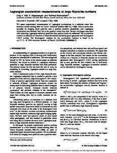
(a) Re = 100

(b) Re = 200

(c) Re = 300

(d) Re = 400

(e) Re = 500

(f) Re = 600

(g) Re = 700

(h) Re = 800

(i) Re = 900

(j) Re = 1000 Figure (3): The steady state streamlines for different Reynolds numbers move to the center of the cavity with the increase in Reynolds number while the two side vortices increase in size as shown in Fig. 4. The streamlines at the top of the cavity also show a high gradient of the tangential velocity which is a characteristic of the lid-driven cavity flow.

4. Numerical results The MRT LBM is used in the simulation of steady viscous incompressible flow in a 2D lid-driven cavity at a range of Reynolds number between 100 and 1000. The flow Reynolds number is calculated based on the cavity width and the velocity of the top lid as a characteristic velocity. The no-slip boundary condition is used for the two side boundaries and the bottom of the cavity. For the top boundary, the normal velocity is set to zero while the tangential velocity is set based on the required Reynolds number. The initial flow field is set to zero velocity for all points inside the cavity. The streamlines for some of the cases are shown in Fig. 3. The figures show the variation in the size and location of the vortices with the Reynolds number. The main vortex tends to

112

Mohammed A. Boraey Mugla Journal of Science and Technology, Vol 3, No 2, 2017, Pages 110-115 The vertical velocity component profiles at y=50 are shown in Fig. 7.

Figure (4): The location of the center of the main vertex as a function of the Reynolds number. Horizontal velocity component profiles at x=50 for different Reynolds numbers are shown in Fig. 5. The figure confirms the high gradient of the tangential velocity component near the top lid region.

Figure (7): Vertical velocity component profiles at y=50 (in LBM units). In contrast to the section at x=50. The horizontal velocity component at y=50 is smaller than the vertical ones since the streamlines are almost vertical at this section of the cavity as can be seen from Fig. 8.

Figure(5): Horizontal velocity component profiles at x=50 (in LBM units). At this vertical plan (x=50) the vertical velocity component is much smaller than the horizontal one which is evident from Fig. 6.

Figure (8): Horizontal velocity component profiles at y=50 (in LBM units). To test the accuracy of the simulation results, the location of the main vortex and the two side vortices are compared against published results. Table (1) shows this comparison for selected Reynolds numbers. As the table shows, the predicted vortices locations are in a perfect match with the published results using other numerical methods which confirm the validity of the results and its suitability to be used as verification for other numerical methods for fluid flow simulation.

Figure (6): Vertical velocity component profiles at x=50 (in LBM units).

113

Mohammed A. Boraey Mugla Journal of Science and Technology, Vol 3, No 2, 2017, Pages 110-115 Table (1): The location of the primary vortex and the two side vortices for Re=100,400& 1000 using the MRT LBM compared to published results (Ref. [14, 15,29-31]).

of the simulation results were confirmed by comparing the results to published results in literature. The simulation results include the steady-state streamlines, horizontal and vertical velocity component profiles at the mid-horizontal and mid-vertical plans of the cavity and the location of the vortices centers (the primary main vortex and the two lower side vortices). This set of results constitutes a detailed dataset that can be used for the testing of new numerical methods in the reported range of Reynolds number. 6. References

Re P [29] [30] [15] [14] [31] MRT

100 400 1000 X Y X Y X Y 0.619 0.738 0.557 0.600 0.544 0.563 0.617 0.734 0.555 0.606 0.531 0.563 0.620 0.737 0.561 0.608 0.533 0.565 0.617 0.742 0.557 0.607 0.529 0.564 0.613 0.738 0.550 0.613 0.525 0.563 0.621 0.742 0.559 0.606 0.533 0.565 (a) Primary vortex (P) Re 100 400 1000 R X Y X Y X Y [29] 0.938 0.056 0.888 0.119 0.863 0.106 [30] 0.945 0.063 0.891 0.125 0.859 0.109 [15] 0.945 0.063 0.890 0.126 0.867 0.114 [14] 0.942 0.050 0.886 0.114 0.864 0.107 [31] 0.938 0.063 0.888 0.125 0.863 0.113 MRT 0.946 0.057 0.887 0.122 0.868 0.113 (b) Lower right vortex (R) Re 100 400 1000 L X Y X Y X Y [29] 0.038 0.031 0.050 0.050 0.075 0.081 [30] 0.031 0.039 0.051 0.047 0.086 0.078 [15] 0.039 0.035 0.055 0.051 0.090 0.078 [14] 0.033 0.025 0.050 0.043 0.086 0.071 [31] 0.038 0.038 0.050 0.050 0.088 0.075 MRT 0.033 0.033 0.049 0.046 0.082 0.076 (c) Lower left vortex (L) Finally, the location of the vortices centers (the primary and the two side ones) for all the simulated cases are given in table (2). This data can be used to accurately assess the accuracy of any numerical method for the range of Reynolds numbers 100 to 1000.

[1].

[2].

[3].

[4].

[5].

[6].

Table (2): The location of the primary vortex and the two side vortices using the MRT LBM Vortex Primary Right Left Re X Y X Y X Y 100 0.621 0.742 0.946 0.057 0.033 0.033 200 0.619 0.681 0.915 0.102 0.033 0.032 300 0.577 0.628 0.896 0.118 0.042 0.040 400 0.559 0.606 0.887 0.122 0.049 0.046 500 0.549 0.594 0.882 0.122 0.057 0.052 600 0.544 0.585 0.878 0.119 0.065 0.057 700 0.540 0.578 0.875 0.118 0.071 0.062 800 0.538 0.573 0.872 0.116 0.076 0.067 900 0.535 0.568 0.870 0.115 0.079 0.072 1000 0.533 0.565 0.868 0.113 0.082 0.076

[7].

[8].

[9].

[10].

5. Conclusion Steady laminar viscous incompressible flow of a Newtonian fluid inside a lid-driven cavity is modeled using the Multi-Relaxation-Time Lattice Boltzmann Method. The simulations were carried out for the range of Reynolds numbers between 100 and 1000. The goal of these simulations is to provide a set of data for the lid-driven cavity flow for benchmarking purposes. The use of MRT LBM offers many advantages over other traditional numerical modeling techniques. These advantages include its explicit nature, the ability to deal with complex boundaries and its suitability for parallel computing. The validity and accuracy

[11].

[12].

114

Witherden, F.D. and A. Jameson. Future Directions of Computational Fluid Dynamics. in 23rd AIAA Computational Fluid Dynamics Conference. 2017. Li, Y., et al., Coupled computational fluid dynamics/multibody dynamics method for wind turbine aero-servo-elastic simulation including drivetrain dynamics. Renewable Energy, 2017. 101: p. 1037-1051. Rutkowski, D.R., et al., Surgical planning for living donor liver transplant using 4D flow MRI, computational fluid dynamics and in vitro experiments. Computer Methods in Biomechanics and Biomedical Engineering: Imaging & Visualization, 2017: p. 1-11. Fortunato, L., et al., In-situ assessment of biofilm formation in submerged membrane system using optical coherence tomography and computational fluid dynamics. Journal of Membrane Science, 2017. 521: p. 84-94. Boulard, T., et al., Modelling of micrometeorology, canopy transpiration and photosynthesis in a closed greenhouse using computational fluid dynamics. Biosystems Engineering, 2017. 158: p. 110-133. Tao, Y., K. Inthavong, and J. Tu, Computational fluid dynamics study of human-induced wake and particle dispersion in indoor environment. Indoor and Built Environment, 2017. 26(2): p. 185-198. Mahmood, R., et al., Numerical Simulations of the Square Lid Driven Cavity Flow of Bingham Fluids Using Nonconforming Finite Elements Coupled with a Direct Solver. Advances in Mathematical Physics, 2017. Abu-Nada, E. and A.J. Chamkha, Mixed convection flow of a nanofluid in a lid-driven cavity with a wavy wall. International Communications in Heat and Mass Transfer, 2014. 57: p. 36-47. 9. Botella, O. and R. Peyret, Benchmark spectral results on the lid-driven cavity flow. Computers & Fluids, 1998. 27(4): p. 421-433. Grillet, A.M., et al., Modeling of viscoelastic lid driven cavity flow using finite element simulations. Journal of Non-Newtonian Fluid Mechanics, 1999. 88(1): p. 99131. Benyahia, S., et al., Simulation of particles and gas flow behavior in the riser section of a circulating fluidized bed using the kinetic theory approach for the particulate phase. Powder Technology, 2000. 112(1): p. 24-33. Alex, J., et al., Analysis and design of suitable model structures for activated sludge tanks with circulating flow. Water science and technology, 1999. 39(4): p. 5560.

Mohammed A. Boraey Mugla Journal of Science and Technology, Vol 3, No 2, 2017, Pages 110-115 [13].

[14].

[15].

[16].

[17].

[18].

[19].

[20].

[21].

[22].

[23].

[24].

[25].

[26].

[27].

[28].

Perumal, D.A. and A.K. Dass, Application of lattice Boltzmann method for incompressible viscous flows. Applied Mathematical Modelling, 2013. 37(6): p. 40754092. Schreiber, R. and H.B. Keller, Driven cavity flows by efficient numerical techniques. Journal of Computational Physics, 1983. 49(2): p. 310-333. Hou, S., et al., Simulation of Cavity Flow by the Lattice Boltzmann Method. Journal of Computational Physics, 1995. 118(2): p. 329-347. Chen, S. and G.D. Doolen, LATTICE BOLTZMANN METHOD FOR FLUID FLOWS. Annual Review of Fluid Mechanics, 1998. 30(1): p. 329-364. He, Y., et al., Lattice Boltzmann method and its applications in engineering thermophysics. Chinese Science Bulletin, 2009. 54(22): p. 4117. Li, Q., et al., Lattice Boltzmann methods for multiphase flow and phase-change heat transfer. Progress in Energy and Combustion Science, 2016. 52: p. 62-105. Bao, J. and L. Schaefer, Lattice Boltzmann equation model for multi-component multi-phase flow with high density ratios. Applied Mathematical Modelling, 2013. 37(4): p. 1860-1871. Psihogios, J., et al., A Lattice Boltzmann study of nonnewtonian flow in digitally reconstructed porous domains. Transport in Porous Media, 2007. 70(2): p. 279-292. Wang, C.-H. and J.-R. Ho, A lattice Boltzmann approach for the non-Newtonian effect in the blood flow. Computers & Mathematics with Applications, 2011. 62(1): p. 75-86. Hao, J. and L. Zhu, A lattice Boltzmann based implicit immersed boundary method for fluid–structure interaction. Computers & Mathematics with Applications, 2010. 59(1): p. 185-193. Yang, J. and E.S. Boek, A comparison study of multicomponent Lattice Boltzmann models for flow in porous media applications. Computers & Mathematics with Applications, 2013. 65(6): p. 882-890. Fakhari, A., D. Bolster, and L.-S. Luo, A weighted multiple-relaxation-time lattice Boltzmann method for multiphase flows and its application to partial coalescence cascades. Journal of Computational Physics, 2017. 341: p. 22-43. Zhuo, C. and P. Sagaut, Acoustic multipole sources for the regularized lattice Boltzmann method: Comparison with multiple-relaxation-time models in the inviscid limit. Physical Review E, 2017. 95(6): p. 063301. Hu, Y., et al., A multiple-relaxation-time lattice Boltzmann model for the flow and heat transfer in a hydrodynamically and thermally anisotropic porous medium. International Journal of Heat and Mass Transfer, 2017. 104: p. 544-558. Liu, Q., Y.-L. He, and Q. Li, Enthalpy-based multiplerelaxation-time lattice Boltzmann method for solidliquid phase-change heat transfer in metal foams. Physical Review E, 2017. 96(2): p. 023303. Bhatnagar, P.L., E.P. Gross, and M. Krook, A model for collision processes in gases. I. Small amplitude processes in charged and neutral one-component systems. Physical review, 1954. 94(3): p. 511.

[29].

[30].

[31].

115

Vanka, S.P., Block-implicit multigrid solution of NavierStokes equations in primitive variables. Journal of Computational Physics, 1986. 65(1): p. 138-158. Ghia, U., K.N. Ghia, and C.T. Shin, High-Re solutions for incompressible flow using the Navier-Stokes equations and a multigrid method. Journal of Computational Physics, 1982. 48(3): p. 387-411. Gupta, M.M. and J.C. Kalita, A new paradigm for solving Navier–Stokes equations: streamfunction–velocity formulation. Journal of Computational Physics, 2005. 207(1): p. 52-68.