Simulation of the Multivariate Generalized Hyperbolic Distribution using Adaptive Importance Sampling Marco Bee and Roberto Benedetti
Abstract In this paper we use Adaptive Importance Sampling for simulating the multivariate Generalized Hyperbolic Distribution and computing tail probabilities. Adaptive Importance Sampling is an extension of classical Importance Sampling that updates sequentially the instrumental density at each iteration. Under the only condition that the density is known in closed form, the method can be used for sampling multivariate distributions and estimate quantities of interest. Some simulations experiments and a real-data application show that, for the problem at hand, the method has an excellent performance, which makes this technique an appealing alternative to more traditional sampling algorithms, whose implementation for the simulation of the Generalized Hyperbolic Distribution is not straightforward. Key words: Statistical computing, Statistical analysis of financial data, Importance sampling
1 Introduction The Family of Generalized Hyperbolic Distributions (GHD), first introduced by Barndorff-Nielsen (1977), has recently been the object of considerable interest. From the theoretical point of view, the main reason is that each GHD is the marginal distribution of a L´evy process; in other words, the value of the increment of the process over a fixed time interval has that distribution. This result is particularly relevant for financial applications, because L´evy processes are often used as continuous-time models of asset prices. On the empirical side, the interest is mostly related to the ability at modelling fat-tailed distributions. Maximum likelihood estimation of the parameters can be performed by means of the EM algorithm (Protassov, 2004). Marco Bee, Department of Economics, University of Trento, via Inama 5, e-mail:
[email protected] ⋅ Roberto Benedetti, Department of Business, Statistical, Technological and Environmental Sciences, University ‘G. d’Annunzio’ of Chieti-Pescara, e-mail:
[email protected]
1
2
Marco Bee and Roberto Benedetti
Generalized Hyperbolic Distributions can be represented as elliptically symmetric variance-mean normal mixtures: if x is a random vector with the p-variate GHD, denoted as x ∼ GHD p (λ γ , β , µ , δ , ∆ ), the conditional distribution of x∣z is N p (µ + zβ ∆ , z∆ ), where z ∼ GIG(λ , δ , γ ) and GIG stands for Generalized Inverse Gaussian. According to this representation, the standard way of simulating the pvariate GHD is based on the following two steps: (i) simulate an observation z from the GIG distribution; (ii) simulate a N p (µ + zβ ∆ , z∆ ) variate. However, simulating the GIG is not straightforward (see Dagpunar, 1989), so that this method is rather cumbersome. In this paper we use a recent extension of Importance Sampling, called Adaptive Importance Sampling (IS) for simulating the multivariate GHD. Adaptive IS was first introduced by Capp´e et al. (2004). Capp´e et al. (2008) extended it to general mixture classes, and Wraith et al. (2009) propose an interesting application. The method is an extension of standard IS because, at each iteration, a sample is simulated from the instrumental density and used to improve the IS density itself. So, ‘adaptivity’ means that the instrumental density sequentially provides a progressively better approximation of the target density. Basically, the only requirement is that the density can be written in closed form. The paper is organized as follows. Section 2 introduces the statistical methods used in the paper, namely standard Importance Sampling and Adaptive Importance Sampling, and reviews the GHD. Section 3 presents the results of the simulation experiments as well as a real-data application. Finally, Section 4 concludes.
2 Methodology Importance Sampling (see Casella and Robert, 2004, Sect. 3.3 for a review) is a variance reduction technique. Instead of simulating observations from the distribution of interest f as in crude Monte Carlo (MC), IS samples an instrumental distribution g that assigns “more weight” to the event of interest. The features of g are crucial for the properties of the estimator, but unfortunately there is no general, readily available procedure for finding the optimal instrumental density.
2.1 Adaptive Importance Sampling Adaptive Importance Sampling (or Population Monte Carlo) is a sampling algorithm first proposed in a Bayesian setup by Capp´e et al. (2004). The idea is that, instead of using a fixed IS density g, one can use a sequence of importance densities g(t) (t = 1, . . . , T ), aimed at approximating the target density f . The general formulation of the algorithm is as follows:
Simulation of the Multivariate Generalized Hyperbolic Distribution
3
1. Simulate a first sample xn = (x1 , . . . , xn )′ ∼ g(1) by means of standard IS; compute (1) (1) (1) the IS weights w j = f (x j )/g(1)(x j ) ( j = 1, . . . , n). 2. Use this sample to approximate the moments of f and construct the updated importance function g(2) . 3. Measure the goodness of the approximation by means of the relative entropy (or Kullback-Leibler divergence; see Rubinstein and Kroese, 2004, Sect. 3.3) from the target: ( ) ∫ f (x) K( f ∣∣g(2) ) = log (2) f (x)dx. (1) g (x) 4. ‘Adjust’ g(2) so that K( f ∣∣g(2) ) ≤ K( f ∣∣g(1) ). Formally, compute minθ K( f ∣∣g(2) ), where θ is the vector of parameters of g(2) . 5. Repeat the preceding steps until some convergence criterion is met. The first important issue is the choice of the functional form of g, which should be flexible enough to allow for a close match of the target and a reasonably easy minimization of (1). According to Capp´e et al. (2004, 2008), a convenient choice is a finite mixture of normal distributions, namely g(t) (x) = g(x; π (t) , θ (t) ) =
D
∑ πd
(t)
(t)
φd (x; θ d ),
(2)
d=1 (t)
(t)
where π (t) = (π1 , . . . , πD )′ is the vector of weights of the D mixture components and θ (t) is a D × 2 matrix whose i-th row contains the parameters of the i-th normal (t) (t) (t)2 density, i.e. θ i = (µi , σi ). If the target density is p-variate (p ≥ 2), (2) is a p-variate normal mixture and the dimensions of θ change accordingly. For the present application, the most interesting result is that an approximate sample from the target density can be obtained by sampling with replacement from g(t) and weighting the observations by means of w(t) . A convenient convergence diagnostic is the so-called normalized perplexity perpn = exp(Hn )/n, where Hn = − ∑nj=1 ω¯ j log(ω¯ j ) is the Shannon entropy of the normalized weights ω¯ j . It can be shown (Capp´e et al., 2008, sect. 2.1) that perpn is an estimator of exp(K( f ∣∣g) and that is included in the interval [0, 1]. Moreover, Capp´e et al. (2008) prove that, as n → ∞, the algorithm monotonically decreases the cross-entropy (1). Thus, it seems plausible to stop the algorithm when the normalized perplexity cannot be further increased (so that the entropy cannot be further decreased). Therefore, monitoring the perplexity over some (say 5) successive iterations, we can stop the algorithm when the normalized perplexity does not change significantly or a predefined ‘large’ number of iterations M is reached. From the technical point of view, the fundamental issue is the update of the importance function g at each iteration. When g is a multivariate normal mixture, the relevant equations are derived by Capp´e et al. (2004). At iteration t, the importance (t) (t) weights associated to the sample (x1 , . . . , xn ) are given by
4
Marco Bee and Roberto Benedetti (t)
(t) wj
=
f (x j ) (t)
(t)
(t)
(t)
∑D d=1 πd φ (x j ; µ d , Σ d ) (t)
(t)
,
j = 1, . . . , n,
(t)
and the normalized weights are w¯ j = w j / ∑nj=1 w j . The update is performed iterating, for any i = 1, . . . , D, the following equations: (t+1)
πi
n
=
∑ w¯ n
(t)
(t)
τi (x j ; π (t) , µ (t) , Σ (t) ),
(3)
j=1
(t)
(t) (t)
(t+1) µi
=
∑nj=1 w¯ n x j τi (x j ; π (t) , µ (t) , Σ (t) ) (t+1)
πi (t)
(t+1) Σi
=
(t)
(t+1)
∑nj=1 w¯ j (x j − µ i
(t)
,
(t+1) ′ (t) ) τi (x j ; π (t) , µ (t) , Σ (t) )
)(xn − µ i
(t+1)
πi
where
τi (x; π , µ , Σ ) =
πi φ (x; µ i , Σ i ) . D ∑d=1 πd φ (x; µ d , Σ d )
(4)
,
(5)
(6)
2.2 The Multivariate Generalized Hyperbolic Distribution A random vector X is said to have a multivariate GHD(λ , α , β , µ , δ , ∆ ) if its density is given by: ⎛√ ⎞λ −p/2 2 + (x − µ )′ ∆ −1 (x − µ ) δ ⎝ ⎠ f (x; λ γ , β , µ , δ , ∆ ) = (2π )−p/2 ⋅ δ γ 2 + β ′∆ β (√ ) exp{(x − µ )′ β } ⋅Kλ −p/2 , (δ 2 + (x − µ )′ ∆ −1 (x − µ ))(γ 2 + β ′ ∆ β ) ⋅ Kλ (δ γ ) √ where δ > 0 and γ = α 2 − β ′ ∆ β ≥ 0 are scalars, β , µ ∈ ℝ p , α 2 ≥ β ′ ∆ β , ∆ is a p × p positive definite symmetric matrix with det(∆ ) = 1 (to avoid identifiability problems) and Kλ (x) is the modified Bessel function of the third kind of order λ . The distribution is generalized because, according to the values taken by λ , one gets several distributions known by different names: see McNeil et al. (2005, p. 80) for details. A major step towards the implementation of the GHD in practical applications was the development of Maximum Likelihood Estimation by means of the EM algorithm (Protassov, 2004). ( γ )λ
Simulation of the Multivariate Generalized Hyperbolic Distribution
5
2.3 Adaptive Importance Sampling for the simulation of the GHD The implementation of Adaptive IS for the simulation of the GHD requires to derive the updating equations resulting from the minimization of the cross-entropy (1). The algorithm based on Gaussian mixtures works as follows. 1. Choose the instrumental density g(1) = ∑D d=1 πd φ (µ d , Σ d ), i.e. the parameters D, π , µ i , Σ i (i = 1, . . . , D). (1) (1) 2. Simulate x1 , . . . , xn independently from g(1) . (1) (1) (1) (1) (1) 3. Compute the importance weights w j = f (x1 j , . . . , x p j )/g(x1 j , . . . , x p j ) ( j = 1, . . . , n), where f is the GHD p density function. For t ≥ 1: 4. Update the importance function to g(t+1) using equations (3) to (6) and the pre(t) (t) (t) (t) vious weighted sample (x1 , w1 ), . . . , (xN , wN ). (t+1) (t+1) 5. Simulate x1 , . . . , xN independently from g(t+1) ; (1) 6. Compute the importance weights w j ( j = 1, . . . , n); 7. Go back to step 4.
3 Simulation and application The choice of the mixture parameters D, π , µ i and Σ i (i = 1, . . . , D), of the sample size n, and of the maximum number of iterations M depends on several factors. To assess their impact in the present setup, we perform some simulation experiments. First we fit a five-variate GHD to a sample of log-returns of five financial time series. The data are the exchange rates of the Swiss Franc (CHF), US Dollar (USD), English Pound (GBP), Canadian Dollar (CAD) and Japanese Yen (JPY) against the Euro. The time horizon is from January 1, 1990 to December 31, 2009. The MLEs obtained by means of the EM algorithm (Protassov, 2004) are as follows:
µˆ = (0.0003, −7.89 ⋅ 10−5, −0.0003, −0.0007, 0.0006)′, βˆ = (−35.0977, −2.6307, 17.2315, 12.1250, −12.5377)′, δˆ = 0.0043, γˆ = 300.8946, ⎞ ⎛ 0.299 0.023 0.021 −0.038 0.252 ⎜ 0.023 1.990 0.742 1.309 1.274 ⎟ ⎟ ⎜ ⎟ ˆ ∆ =⎜ ⎜ 0.021 0.742 1.082 0.646 0.511 ⎟ . ⎝ −0.038 1.309 0.646 2.202 0.760 ⎠ 0.252 1.274 0.511 0.760 2.613 Using only the first two variables, namely CHF and USD, we get:
(7)
6
Marco Bee and Roberto Benedetti
µˆ = (0.0002, −0.0002)′, δˆ = 0.0029,
βˆ = (−35.716, 6.094),′ ( ) 0.385 0.047 ˆ γˆ = 301.4950, ∆ = . 0.047 2.602
(8)
0.020
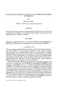
Fig. 1(a) displays the contour plot of the GHD2 density with the parameters in (8) and of the instrumental density; Fig. 1(b) displays 1000 simulated observations from the GHD2 . The IS density is the best-fitting bivariate normal mixture, obtained by means of the Adaptive IS procedure, with n = 10 000; the algorithm stops after a number of iterations equal to min{20,t ∗), where t ∗ > 5 is such that (i) ( j) maxi, j∈{t ∗ ,t ∗ −1,...,t ∗ −5} ∣perpn − perpn ∣ < ε , with ε = 0.001. With D = 7, the quality of the approximation is very good, with a maximum perplexity equal to 0.9943.
−0.015
−0.04
−0.02
−0.005 0.000
0.00
0.005
0.02
0.010
0.015
0.04
GHD2 density Best fitting mixture
−0.006
−0.002
0.002
0.006
−0.015
−0.005
0.005
0.015
Fig. 1 (a) Contours of the GHD2 density and of the best fitting Gaussian mixture; (b) 1000 observations sampled from the best-fitting mixture.
Simulation of the Multivariate Generalized Hyperbolic Distribution
7
Next we apply the Adaptive IS procedure to the 5-variate distribution with the parameters in (7). In this case, we perform a small simulation study, consisting in replicating the procedure B = 50 times. Fig. 2 displays the boxplots of the perplexities obtained in the first 10 iterations; ‘Failure rate’ is the ratio ‘{number of replications in which the algorithm did not converge}/{total number of replications}. The initialization is the same in all cases. Whereas the four graphs are approximately similar, there is a considerable difference in the failure rate. We can therefore conclude that, when p increases, a large sample size is of crucial importance. When n is small, it often happens that the algorithm breaks down, typically because the covariance matrix of one of the populations becomes singular.
1.0 0.8
0.8
0.6
0.6 0.4 0.2
0.0
1.0
0.4
(b) n = 4000; Failure rate = 0.25
0.2
(a) n = 3000; Failure rate = 0.33
0.0 2
4
6
8
10
2
(c) n = 5000; Failure rate = 0.15
4
6
8
10
(d) n = 10000; Failure rate = 0.06
1.0
1.0
0.8
0.8
0.6
0.6
0.4
0.4
0.2
0.2 0.0
0.0 2
4
6
8
10
2
4
6
8
10
Fig. 2 Normalized perplexity estimates for the first 10 iterations of the algorithm over 50 simulation replications. The distributions are shown as boxplots. The thick horizontal line is the median, the box is the interquartile range (IQR), containing 50% of the points; the whiskers correspond to the interval 1.5 ⋅ IQR from either Q1 (lower) or Q3 (upper); points outside the interval [Q1,Q3] (outliers) are represented as circles. ‘Failure rate’ is the ratio ‘{number of replications in which the algorithm did not converge}/{total number of replications}.
8
Marco Bee and Roberto Benedetti
Finally, we compute the joint tail probability p = P(r1 < c1 , r2 < c2 , r3 < c3 , r4 < c4 , r5 < c5 ) for the logarithmic returns of the exchange rates at hand, using n = 10 000 and various thresholds ci (i = 1, . . . , 5). The results are displayed in Table 1. Table 1 Joint tail probability p = P(r1 < c1 , r2 < c2 , r3 < c3 , r4 < c4 , r5 < c5 ) for the 5-dimensional data and various thresholds. c
(0, 0, 0, 0, 0)
−(2, 2, 2, 2, 2) ⋅ 10−3
−(5, 2, 2, 2, 5) ⋅ 10−3
−(5, 2, 5, 2, 10) ⋅ 10−3
p
0.0348
0.0062
0.0024
4 ⋅ 10−4
4 Conclusion In this paper we have used Adaptive Importance Sampling to simulate the multivariate Generalized Hyperbolic Distribution and compute joint tail probabilities for some exchange rates. Both the simulation experiments and the empirical application showed that the procedure guarantees a very precise approximation. For smalldimensional problems, even a rather small sample size produces good results; when the dimension increases, a larger sample size is necessary. This approach seems to be a convenient and general solution for the simulation of non-standard multivariate distributions with known density.
References 1. Barndorff-Nielsen O.E.: Exponentially decreasing distributions for the logarithm of the particle size. Proceedings of the Royal Society. London. Series A. Mathematical and Physical Sciences 353, 401-419 (1977). 2. Capp´e, O., Guillin, A., Marin, J., Robert, C.P.: Population Monte Carlo. Journal of Computational and Graphical Statistics. 13, 907-929 (2004). 3. Capp´e, O., Douc, R., Guillin, A., Robert, C.P.: Adaptive Importance Sampling in general mixture classes. Statistics and Computing. 18, 447-459 (2008). 4. Dagpunar, J.S.: An easily implemented Generalized Inverse Gaussian generator. Communications in Statistics - Simulations. 18, 703-710 (1989). 5. Protassov, R.S.: EM-based maximum likelihood parameter estimation for multivariate generalized hyperbolic distributions with fixed λ . Statistics and Computing. 14, 67-77 (2004). 6. Wraith, D., Kilbinger, M., Benabed, K., Capp´e, O., Cardoso, J.-F., Fort, G., Prunet, S., Robert, C.P.: Estimation of cosmological parameters using adaptive importance sampling. Physical Review D. 80, 023502. (2009).