simulation study of a dynamic agv-container job ... - CiteSeerX

1

SIMULATION STUDY OF A DYNAMIC AGV-CONTAINER JOB DEPLOYMENT SCHEME By Cheng Yong Leong B.Eng. Electrical Engineering National University of Singapore, 2000

SUBMITTED TO THE SMA OFFICE IN PARTIAL FULFILLMENT OF THE REQUIREMENTS FOR THE DEGREE OF MASTER OF SCIENCE IN HIGH PERFORMANCE COMPUT ATION FOR ENGINEERED SYSTEMS AT THE SINGAPORE-MIT ALLIANCE JUNE 2001

Signature of Author: Cheng Yong Leong ___________________________________________________________ High Performance Computation for Engineered Systems June 30, 2001

Certified by: ________________________________________________________________ Assoc. Prof. Teo Chung Piaw SMA HPCES Fellow Project Supervisor Accepted by: ________________________________________________________________ Assoc. Prof. Khoo Boo Cheong Programme Co-Chair HPCES Programme Accepted by: ________________________________________________________________ Prof. Jaime Peraire Programme Co-Chair HPCES Programme

2

ACKNOWLEDGEMENTS The author will wish to thank his advisor Prof. Teo Chung Piaw whose expert advice has helped in the completion of the project. His guidance and comments has aided in looking into the finer aspects of the simulation and in obtaining meaningful results.

The author will wish to thank Mr. Loy Hein Thuan, Manager, Operations Planning Department, PSA Corp., for providing the opportunity to work on this problem. The author is grateful to PSA Corp for providing the resources to do the simulation work.

The author will also wish to thank Dr. Tan Kok Choon, Manager, Operations Planning Department, PSA Corp. for providing the author with advice for this problem.

The author will like to thank the PSA Corp. AGV team comprising of Mr. Lee Tat Wee, Senior Systems Analyst, Container Terminal Systems Department, Mr. Ricky Seng

Siang

Ping,

Senior

Operations

Research

Officer,

Operations

Planning

Department and Mr. Gabriel Lau, Deputy Manager (Ship Operations Systems), Container Terminal Systems Department for proposing this project. The author will also wish to thank SMA for the support in doing this project.

Last but not the least the author will like to thank all the SMA students, which make the stay in SMA more memorable. Author 15th June 2001

3

TA B L E 1

OF

C ONTENTS

INTRODUCTION......................................................................................................9 1.1

BACKGROUND OF CONTAINER TERMINAL OPERATION...................................9

1.2

AUTOMATED GUIDED VEHICLES (AGV S) ..................................................... 10

1.3

PSA PORT AUTOMATION PROJECT (PPAP) .................................................. 11

1.4

PROBLEM STATEMENT .................................................................................. 12

1.5

PROJECT CONTRIBUTION ............................................................................... 14

1.6

OUTLINE OF THE THESIS .............................................................................. 14

2

LITERATURE REVIEW .......................................................................................15

3

CURRENT DEPLOYMENT SCHEME................................................................ 18

4

3.1

THEORETICAL INSIGHT BEHIND PMDS ......................................................... 18

3.2

DESIGN OF THE PMDS MODEL ...................................................................... 20

PROPOSED DEPLOYMENT SCHEME ..............................................................23 4.1

PROBLEM FORMULATION OF THE PROPOSED DEPLOYMENT SCHEME.............. 23

4.1.1

4.2 5

4.1.1.1

Arc cost of arcs flowing from AGV to container node .................... 27

4.1.1.2

Arc cost of arcs flowing from container i’ to container j node ........ 28

DESIGN OF THE PROPOSED DEPLOYMENT SCHEME MODEL............................. 30

DEADLOCK PREDICTION & AVOIDANCE ALGORITHM .........................33 5.1

THE CONDITIONS LEADING TO A DEADLOCK ................................................. 33

5.2

TYPES OF DEADLOCK IN THE AGVS ................................................................ 34

5.3

METHODS IN PREDICTING OR DETECTING CYCLIC DEADLOCK ....................... 35

5.4

PROPOSED DEADLOCK PREDICTION STRATEGY .............................................. 35

5.5

PROPOSED DEADLOCK AVOIDANCE STRATEGY .............................................. 38

5.5.1 6

Calculation of Non-zero Arc Costs ........................................................... 26

One-zone step deadlock resolution ........................................................... 39

IMPLEMENTATION .............................................................................................40 6.1

AUTOMOD SIMULATION SOFTWA RE .............................................................. 40

6.2

SPECIFICATIONS OF THETWO MODELS .......................................................... 40

6.3

DETERMINATION OF THE EXPECTED VALUES OF AVERAGE VELOCITY OF THE

VEHICLES .................................................................................................................. 41

6.4 7

C-CODES AND INTERFACING.......................................................................... 42

RESULTS AND DISCUSSION ..............................................................................44

4

7.1

SCHEMATICS OF THE SIMULATION MODEL LAYOUT ....................................... 44

7.2

COMPARISON OF EFFECTS OF THE NUMBER OF AGVS ................................... 45

7.3

EFFECT OF THE VARIATION OF TIME WINDOW............................................... 48

7.4

DISCUSSIONS AND CONCLUSIONS ................................................................. 50

8

REFERENCES .........................................................................................................52

9

APPENDIX A...........................................................................................................54 9.1

MINIMUM COST FLOW (MCF) CODE ............................................................. 54

5

L IST

OF

F IGURES

Figure 1.1: A prototype of AGV used by PSA Corp. .................................................. 11 Figure 1.2:Part of the PSA simulation model showing routing on one berth. ............. 12 Figure 3.1:Illustration of a typical schedule of job deployment .................................. 19 Figure 3.2:Illustration of the selection of an AGV to dispatch a job ........................... 20 Figure 3.3:An example of the assignment of the appointed pickup/drop off time for 8 jobs....................................................................................................................... 21 Figure 3.4:A visualization of the current deployment scheme .................................... 22 Figure 4.1:Example of a network of 2 AGVs and 4 containers using formulation (N1) .............................................................................................................................. 25 Figure 4.2:Example of a network of 2 AGVs and 4 containers using formulation (N2) .............................................................................................................................. 26 Figure 4.3:Illustration of the calculation of the distance traveled for the 4 cases ....... 29 Figure 4.4: An assignment example of appointed time for 10 jobs for 1 crane........... 31 Figure 5.1:A cyclic deadlock formed by the vehicles .................................................. 33 Figure 5.2:Flowchart of the one-zone step deadlock prediction algorithm ................. 36 Figure 5.3: Illustration of one-zone step deadlock prediction ..................................... 36 Figure 6.1: Illustration of the C interface with the AutoMod model for the mcf model .............................................................................................................................. 43 Figure 7.1: Layout of the four berths in the simulation model.................................... 44 Figure 7.2:Scenarios showing AGVs picking/dropping jobs in the berth and yard areas .............................................................................................................................. 44

6

L IST

OF

TA B L E S

Table 6.1: List of average velocities of random selection of 10 AGVs....................... 42 Table 6.2:Average velocity for the total number of AGVs used................................. 42 Table 7.1:Total number of boxes serviced in each berth ............................................. 45 Table 7.2:Ship average makespan in hours in each berth for pmds model.................. 45 Table 7.3:Ship average makespan in hours in each berth for mcf model .................... 46 Table 7.4:Average throughput of the ship in each berth for pmds model................... 46 Table 7.5:Average throughput of the ship in each berth for mcf model...................... 46 Table 7.6: Length of time deviations from the appointed service time for pmds model .............................................................................................................................. 47 Table 7.7:Length of time deviations from the appointed service time for mcf model 47 Table 7.8: Improvement of the mean time deviations of mcf model........................... 47 Table 7.9: Total number of boxes serviced in each berth ............................................ 48 Table 7.10:Ship average makespan in each berth for pmds model.............................. 48 Table 7.11:Ship average makespan in each berth for mcf model................................ 48 Table 7.12:Average throughput of the ship in each berth for pmds model................. 49 Table 7.13:Average throughput of the ship in each berth for mcf model.................... 49 Table 7.14:Length of time deviations from the appointed service time for pmds model .............................................................................................................................. 49

7

SIMULATION STUDY OF A DYNAMIC AGV-CONTAINER JOB DEPLOYMENT SCHEME

by

Cheng Yong Leong

Submitted to the SMA office on June 15, 2001 In Partial Fulfillment of the Requirements for the Degree of Master of Science in High Performance Computation for Engineered Systems

ABSTRACT Automated Guided Vehicle (AGV) Container-Job deployment is essentially a vehicle dispatching problem. In this problem, the impact of vehicle dispatching polices on the ship makespan for discharging and/or loading operations is analyzed. In particular, here the storage location of each container is an input to the simulation model and is known. Thus, given a storage location for each container to be discharged from the ship and given the current location of each container to be loaded onto the ship, the problem is how to dispatch vehicles to containers so as to minimize the makespan of the ship so as to increase the throughput. The makespan of the ship refers to the time a ship spends at the port for loading and unloading operations. Automated Guided Vehicle System (AGVS) forms a very important part of automated material handling and its performance affects the efficiency of the entire system. Deadlock formation is a serious problem as it stalls the AGVS. Thus, the objective of this project is to develop an efficient deployment algorithm scheme, which will incorporate and integrate with the deadlock prediction and avoidance algorithm done in previous study [1]. The prediction & avoidance algorithm aims to predict and avoid cyclic deadlock. This project will compare the performance of current deployment scheme used by PSA with the new proposed deployment scheme, both with deadlock prediction & avoidance algorithm. The current deployment scheme, namely PMDS makes use of a greedy heuristics which dispatches the available vehicle that will reach the quay with the minimum amount of time the vehicle has to spend waiting for the crane to discharge or load the container from or onto the ship. The new deployment scheme

8

aims to formulate the problem as a minimum cost flow problem, which will then be solved by network simplex code. The vehicles will then be dispatched based on the solutions obtained. The two simulation models are implemented using discrete-event simulation software, AutoMod, and the performances of both deployment schemes are analyzed. The simulation results show that the new deployment scheme will result in a higher throughput and lower ship makespan than the current deployment scheme. Keywords: Automated Guided Vehicles (AGV), greedy heuristic, minimum cost flow, network formulations, simulation study, deadlocks, one-zone step deadlock prediction and avoidance algorithm, vehicle deployment, job based approach, vehicle based approach

Dissertation Supervisors: 1. Assoc. Prof. Teo Chung Piaw, SMA Fellow, NUS 2. Dr. Tan Kok Choon

Chapter 1

9

Introduction

1 INTRODUCTION In 1966, the first deep-sea container service was introduced for the transport of general cargo. Since then, container shipping has become a common way to move all types of products, especially high-value cargo. Due to decreased costs and lower rates, customer demand, increasingly cost-efficient processes, and globalization of trade, the use of containers for sea-borne cargo has seen a steady increase since its introduction in the mid 1960’s. Container terminals have become an important component of logistics networks. To satisfy demand of customers, it is necessary that container ships are unloaded and loaded quickly. This needs the development of sophisticated, highly automated container transportation systems, which will allow the efficient container movement within the container terminal area.

One of the world’s leading port operators, PSA Corporation based in Singapore, is planning to automate its container transportation within the container terminal by implementing an Automated Guided Vehicle (AGV) System (AGVS) in its new, highly

automated

container

terminal.

Typical

operational

planning

and

control

problems in such system are: dispatching of AGVs to containers in the terminal, routing of AGVs and controlling traffic in the network of lanes and junctions. In this project, we consider one aspect of the terminal operation, which is to dispatch AGVs to containers in the terminal.

1.1

BACKGROUND OF CONTAINER TERMINAL OPERATION

When a vessel arrives at the container terminal for a transshipment operation, containers are first discharged from the vessel onto AGVs by quay cranes; the AGVs then transport the containers to the pre-specified storage locations in the yard area. Typically, after most, or all, containers have been unloaded from the vessel, other containers are uploaded onto the ship. These containers are carried by AGVs from the yard to the quay area, and are loaded onto the ship by quay crane. There are two types of cranes in the terminal: quay cranes, which used to load and unload containers to Simulation Study of AGV-Container job Deployment Scheme

Chapter 1

Introduction

10

and from the ship; and yard crane, used to load and unload containers at the terminal yard storage area. Containers handled by the terminals are in standard size (Twenty-foot-equivalent unit (TEU)) containers. An AGV can carry one TEU or two TEUs. When a container is unloaded from a vessel, it is pickup by a quay crane and drop onto an AGV directly without unloading it onto the ground. Unloading containers onto ground will need additional crane operation to lift it from the ground and load onto the AGV, which will affect the throughput of the whole operation and is not desirable. Thus, an AGV needs to be available by the crane throughout the loading and unloading operations.

A few hours before the arrival of an incoming ship, the terminal receives detail information about its contents; i.e., number and location of containers that are to be discharged into the yard, and a list of containers the have to be uploaded onto the vessel. This information allows the terminal dispatchers to generate a crane job sequence, which specify the orders of the containers that are going to be unloaded from and loaded onto the vessel by each quay crane serving the vessel. The unloading sequence to unload containers from vessel onto the yard is determined by the position of the containers on the vessel, their destinations and contents. Similarly, the uploading sequence to upload containers from the yard to the vessel depends on the content, location and next destination of the containers. The crane job sequence always starts with discharging containers from vessel, followed by the loading containers onto the vessel. From these crane job sequences, each container is given a time window that it must leave its source and reach its destination determined by the working rate of the crane that serve this container.

1.2

AUTOMATED GUIDED VEHICLES (AGVS)

AGVs are driver-less industrial trucks, usually powered by electric motors and batteries. AGVs range in size from carrying small loads of a few kilograms up to loads over 100 tons. The working environment may vary from offices with carpet floor to harbor dockside areas. A prototype of AGV used by PSA Corp. in its highly automated container terminal is shown in Figure 1.1.

Simulation Study of AGV-Container job Deployment Scheme

Chapter 1

Introduction

11

Figure 1.1: A prototype of AGV used by PSA Corp. Modern AGV Systems are now controlled by flexible, on-board microcomputers. System management computers and radio frequency controls are incorporated into the system to optimizing the AGV utilization, giving transport orders, tracking the material in transfer and directing the AGV traffic. Through these advance control systems, the exact location of AGV, speed of AGV and the traffic condition at certain zone are known from time to time. Under this ideal information system, a more efficient dispatching, routing and traffic control strategy could be implemented.

1.3

PSA PORT AUTOMATION PROJECT (PPAP)

PSA Corporation is one of the world’s leading port operators and in Singapore PSA handles more than 17 Million TEU of cargo in the year of 2000. PSA operate many ports outside Singapore and due to increasing demand and also to maintain and improve their quality of service, they resort to automation of port activities. Currently, PSA employs fully automated cranes in their ports as part of their container storageretrieval system. It operates about 24 quay cranes, 44 bridge cranes (which are yard cranes) and 15 gantry cranes at the Pasir Panjang Terminal.

To further improve the service, PSA wants to fully automate their port operation. As part of this automation process, AGV system is introduced to transport containers within port. In Singapore, land is a scarce resource and efficient usage of the available space is one the prime objective in any project. An important feature of the ports in Simulation Study of AGV-Container job Deployment Scheme

Chapter 1

12

Introduction

Singapore is that most of the cargo (almost 80%) is for transshipment. Hence, a sufficient amount of space for transshipment goods must be available close to the dock.

Yard

Side

lanes Traveling lane

Working lane 1

Working lane 2 Corridor Container Storage Area

Berth

Side

lanes

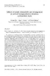
Figure 1.2:Part of the PSA simulation model showing routing on one berth.

To maximize the usage of the land area close to the dock, a complex AGVS layout has been planed for PSA. A part of the layout drawn by PSA is shown in Figure 1.2. The Export/Import containers are stored in the storage yard and the vessels arrive at the berth. All the containers need to be transported to or from vessel and hence there are more lanes in the berth-side. The transshipment containers are stored in the storage yard. A berth is the area between the two corridors. When the layout is complex, the control and navigation systems of the AGVS must be very efficient to deploy AGV to container jobs in the terminal, and prevent any major congestion in the AGV traffic.

1.4

PROBLEM STATEMENT

To design a highly efficient automated container terminal, PSA expressed the need to develop a dynamic AGV dispatching strategy to deploy AGVs to transport containers within the terminal area.


Chapter 1

Introduction

13

The AGV used by PSA has capacity to carry one 40/45 feet container or one 20 feet container or two 20 feet containers. Each container job involves the loading of a container onto the AGV, the movement of the AGV to the destination of the container, and the unloading of the container from the AGV. The following assumptions are used in this project: •

Exact location and impending movement route of an AGV can be accurately retrieved from the AGV Deployment System (ADS).

•

Time needed to travel from each point to another point in the AGVS can be retrieved from the ADS.

•

Source and destination location of all container jobs are given.

•

The time for the unloading container (container to be unloaded from a vessel) to leave the quay crane is generated and given.

•

The time for a loading container (container to be loaded onto a vessel) to reach the quay crane is generated and given.

•

Yard crane resources are always available.

The AGV dispatching problem is to deploy AGVs to serve all the container jobs such that all the time constraints for all jobs are met. This makes sure that an AGV has to reach the quay crane before the time the container is to be dropped off or picked up by the quay crane. If this constraint is satisfied by the deployment scheme, the terminal is operated at a throughput rate that is pre-specified. However, the queuing of AGVs to queue at the quayside is undesirable as it creates congestion at the quayside, hence another objective of the deployment scheme is to reduce the waiting time of the AGVs at the quayside when they are waiting for the quay crane to pickup or drop off containers onto it.

Although an AGV can carry either one or two containers, only the case that an AGV can only carry one container at a time will be studied in the simulation. The project should propose a more optimal deployment scheme for this simulation model and compare the performance of the two deployment schemes.


Chapter 1

1.5

14

Introduction

PROJECT CONTRIBUTION

The problem proposed has been studied in detail and the following chapters provide a detailed description of the problem and the solution proposed. The highlights of the project are: •

Development of an efficient model using a simulation language, AutoMod.

•

Development of the current model using a simulation language, AutoMod.

•

Solving of this model using minimum cost flow algorithm.

•

Integration of both deployment schemes with deadlock prediction and avoidance strategy.

1.6

OUTLINE OF THE THESIS

The remainder of the document is divided into the following chapters. •

Chapter 2 provides a detailed review of the existing literature on vehicle dispatching

using

evolutionary

algorithm,

vehicle

dispatching

in

Flexible

Manufacturing System, vehicle-scheduling algorithms. •

Chapter 3 presents a discussion on the design of the current deployment scheme adopted by PSA.

•

Chapter 4 presents a discussion on the design of the proposed deployment scheme developed using minimum-cost flow algorithm.

•

Chapter 5 presents the deadlock prediction and avoidance measures adopted.

•

In Chapter 6, a detail description of the implementation of the model in AutoMod is provided

•

Chapter 7 provides results obtained in the project and a detail discussion of the results is included.


Chapter 2

15

Literature Review

2 LITERATURE REVIEW Vehicle dispatching strategy is a very important research topic that has been extensively analyzed, mainly in the context of Material Handling System (MHS) control. The majority of these efforts have been centered on Automated Guided Vehicle Systems.

Co [15] dealt with the assignment of transportation equipment to service requests on the shop floor. He assumed a fixed shop layout with predetermined material handling flow paths and fixed transporter fleet size. The problem can be viewed as a vehiclescheduling problem and can be modeled using Mixed Integer Programming. The problem is also similar to the Time Constrained Vehicle Routing Problem (TCVRP) which is proven to be NP-hard.

Egbelu and Tanchoco [17] presented some heuristic rules for dispatching AGVs in a job shop environment. There are two main approaches to the problem: job-based approach and vehicle-based approach. The job-based approach tries to schedule the ‘tightly constrained jobs’ (i.e. with smaller time windows) first. The approach entails selecting the Nearest Vehicle (NV), the Farthest Vehicle (FV), the Longest Idle Vehicle (LIV) or the Least Utilized Vehicle (LUV) to serve the most tightly constrained job. The unloaded movement times of vehicles, which correspond to the sequence dependent set-up times in the scheduling framework, are ignored. The vehicle-based approach, on the other hand tries to minimize the unloaded travel times so that jobs will have more opportunities to be scheduled. Examples of vehicle-based approaches are Shortest Travel Time (STT), Longest Travel Time (LTT), Maximum Outgoing

Queue

Size

(MOQS),

Minimum

Remaining

Outgoing Queue

Space

(MROQS) and First Come First Serve (FCFS) Simchi-Levi et al [3] proposed a vehicle-based dispatching strategy for a mega container terminal. The objective was to minimize the makespan to serve a vessel.


Chapter 2

Literature Review

16

The heuristic proposed deploying vehicles to the earliest possible container jobs once the vehicle is free. The deviation of the proposed heuristic makespan from optimality was also investigated.

Akturk and Yilmaz [18] proposed an algorithm to schedule vehicles and jobs in a decision-making

hierarchy based on mixed integer programming. Their micro-

opportunistic scheduling algorithm (MOSA), combined job-based and vehicle-based approaches into a single algorithm in which critical jobs and travel times of unloaded vehicles are considered simultaneously. However, MOSA is only useful for AGV systems with a small number of jobs and vehicles as the computational time becomes impractical when the job number or the size of the vehicle fleet is large.

A human dispatcher typically performs the assigning of vehicles to jobs. Successful performance of this task requires much experience, judgment and expertise on the part of the scheduler. Hence, Potvin et al [16] suggested the use of a neural network model as a sub-symbolic and empirical means of modeling the decision process of expert dispatchers. As an alternative to using expert systems, Bose et al [19] proposed obtaining an initial solution using either a job-based or vehicle-based approach and subsequently improving it via an evolutionary algorithm. However, these algorithms only perform well for AGV systems with small numbers of jobs and vehicles.

Majority of the above literatures assumed a unit capacity vehicle, which could only take one unit of load at a time. An efficient way to solve a unit capacity vehicle dispatching problem is to first formulate the whole deployment problem as a network flow problem. A network simplex algorithm with an upper bound technique, which is a specialized revised simplex algorithm, can solve the problem efficiently by exploiting the structure of the network flow problem. The linear algebra of the simplex algorithm is replaced by simple network operations. Ahuja, Magnanti, and Orlin [9] describe the (primal) network simplex algorithm and gave pseudo-codes and implementation details. An implementation of the primal and dual network simplex algorithm is presented by Löbel in [13]. In practical applications, besides the vehicle-dispatching problem one must also consider the possible formation of deadlocks in the Automated Guided Vehicle Simulation Study of AGV-Container job Deployment Scheme

Chapter 2

Literature Review

17

System. The deadlock detection and avoidance strategy that has been used in this project is based on the new approach proposed by Wee and Moorthy [1]. The deadlock prediction is a one-zone step prediction algorithm. The avoidance strategy makes use of the “wait and proceed” approach and the semi-dynamic re-routing strategy, which uses the shortest path algorithm to determine the routes for the AGVs.

To evaluate the performance of the deployment schemes, simulation studies are essential. To implement the simulation effectively, prudent steps must be taken to ensure the accuracy of the results presented by the model. A systematic approach to a proper simulation study has been discussed by Banks and Carson in [11] and Law in [12].


Chapter 3

Current Deployment Scheme

18

3 CURRENT DEPLOYMENT SCHEME The current deployment scheme, namely the Prime-Mover Deployment scheme (PMDS), as the name suggests, is derived from the original prime mover deployment scheme which is going to be incorporated into the AGVS where the man-driven prime mover is going to be replaced by the Automated Guided Vehicle (AGV). Each container corresponding to a ship is a job and there are 2 types of job movements, discharging/unloading (movement from quay to yard) and loading (movement from yard to quay). We assume that we are given the crane job sequence for each quay crane serving the ship. The crane job sequence for each quay crane consists of the following information. •

A sequence of jobs that will be discharged from/loaded onto the ship,

•

A set of potential storage locations in the yard area for each container to be discharged from the ship and is already determined.

The job’s pickup location is denoted as the source of the container to be loaded onto the vehicle and the job’s drop off location is denoted as the destination of the container to be unloaded from the vehicle. In this chapter, the insight and the algorithm behind the PMDS model will be discussed

3.1

THEORETICAL INSIGHT BEHIND PMDS

The general rule behind the deployment scheme is based on a greedy heuristic that aims to dispatch vehicles to jobs such that the time each vehicle spends waiting for the quay crane to serve a job is minimized. For each quay crane, the predetermined crane job sequence, consisting of n jobs may consist of only unloading jobs (or “u” job) or only loading jobs (or “l” job) or a combination of both unloading and loading jobs (or “u/l” job). In the latter case, the job sequence consists of two parts: the first part includes all the “u” jobs followed by all the “l” jobs. For each “u” (“l”) job, there is a predetermined drop-off (pickup) point in the yard, which is the location of the job.


Chapter 3

19


In the greedy heuristic, the first k jobs are assigned, each to a single AGV. The next job is assigned to the AGV such that the AGV will reach the location at a time that will minimize the AGV waiting time for the crane to unload/load the “u”/“l” job to the vehicle. Specifically, when assigning a “u” job, the AGV that has the closest arrival time at the quayside to the appointed pickup time of the job will be dispatched to this job. Similarly, when assigning a “l” job, the AGV that has the closest arrival time at the quayside to the appointed drop off time of the job will be dispatched to this job. Normally for “l” job, the AGV that can reach the job source at the yardside at the earliest time is dispatched since it needs to travel a longer distance from current position to the yardside and to the quayside compared to a “u” job.

The deployment scheme focuses on deployment of one job at a time. All the jobs are arranged in the order of First In First Out (FIFO) basis based on the earliest appointed pickup/drop off time of the job at the quayside. A pictorial view of the job schedule is shown in Figure 3.1. Select first Job to dispatch

Current time Time window

Time Job 0 Estimated travel time to destination Job 1 Job 2

Slack/ waiting time

Job 3 Planned job appointed time

Actual job start time

Planned job finished time

Actual job finished time

Figure 3.1:Illustration of a typical schedule of job deployment From Figure 3.1, Job 0 with the earliest appointed pickup/drop off time or the least waiting time (indicated in dotted arrow) will be selected to dispatch first followed by Job 1,2,3 and so on. The length of the time window dictates the time interval between the appointed pickup/drop off times of two jobs. If the job is a “u” job, the start time will be the pickup time and if a job is a “l” job, the start time will be the drop off time. A pictorial view of the selection of a vehicle for deployment is shown in Figure 3.2.


Chapter 3

20


Job i appointed pickup/drop Select a vehicle to dispatch Job i

off time Time

AGV 0

Estimated travel time to quay

Waiting time

AGV 1 AGV. 2 AGV 3 AGV 4 AGV 5 AGV available time

AGV estimated arrival time at the quay

Deployable vehicles Job i time window

Figure 3.2:Illustration of the selection of an AGV to dispatch a job From the illustration in Figure 3.2, AGV3 is selected to dispatch job i since it has the least expected waiting time for the quay crane appointed time to unload or load job i from or to the vehicle.

3.2

DESIGN OF THE PMDS MODEL

The planning of the time to dispatch each job is done in the following manner. The 1st 4 jobs per crane will be assigned an appointed pickup/drop off time first. The fifth job per crane will be assigned when the service of the 1st job at the quay has actually been completed. The assignment of the sixth job will depend on the completion of the 2nd job and so on. The planning period is effectively 4 jobs ahead. For the 1st 4 jobs, the appointed pick/drop off time of the ith job will be Appointed time = ship discharge time + (i-1) * time window For the next subsequent jobs after the 1st four, the appointed pickup/drop off time of the jth job will be Appointed time = (j-4)th actual pickup/drop off time + 4* time window


Chapter 3

21


Thus, for each crane, there are only 4 jobs at each time that are assigned an appointed pickup/drop off time. The assignment of the appointed pickup/drop off time for 8 jobs is illustrated with an example in Figure 3.3.

1

2

12:00am

3

4

5

6

7

8

time

12:02am 12:04am 12:06am

1st job actual pickup 1

2

3

5

4

12:01am 12:02am 12:04am 12:06am

2nd job actual pickup/drop off

3

2

12:09am

4

6

12:02am 12:04am 12:06am

3rd job actual pickup/drop off

4th job actual pickup/drop off

time

time

12:10am

3

4

7

12:03am

12:06am

12:11am

time

4

8

12:05am

12:13am

time

Figure 3.3:An example of the assignment of the appointed pickup/drop off time for 8 jobs Before calculating the expected waiting time, the status of the AGVs must be determined. AGVs can be in the following 4 states, “retrieving”, “delivering”, “going to park ” and “idle or parked” status. Only AGVs that are neither in the state of “retrieving” the next load nor being assigned to the next load are deployed in the current deployment scheme, PMDS. The waiting time for job Li, for the remaining 3 states of the AGV is calculated as follows:

If the job Li is a “u” job, 1.

If the AGV is “delivering” the current job, Lj, Distance traveled by AGV, Dist = distance(AGV current position, Lj destination) + distance(Lj destination, Li source) Waiting time for Li = Li appointed pickup time – (Dist/Average Velocity + crane average operating rate for Lj)


Chapter 3

2.

22


If the AGV is “going to park ”, going towards its assigned park location, Distance traveled by AGV, Dist = distance(AGV current position, AGV destination) + distance(AGV destination, Li source) Waiting time for Li = Li appointed pickup time – Dist/Average Velocity

3.

If the AGV is “idle”, Distance traveled by AGV, Dist = distance(AGV current position, Li source) Waiting time for Li = Li appointed pickup time – Dist/Average Velocity

If the job Li is a “l” job, the value of “Dist” will be increased by another distance(Li source, Li

destination). Moreover, the waiting time will be decremented by another

yard crane average operating rate for Li. The whole deployment scheme can be visualized in Figure 3.4. For job Lj

•AGV 0 •AGV 1 •… •AGV m Vehicle list

•Job L

•AGV k •AGV k+1 •... •AGV j

minimum waiting time Pre-Calculation

Deployable Vehicle list Assigned

j

Select vehicle with

•AGV m

Figure 3.4:A visualization of the current deployment scheme The determination of the average velocity of each AGV is important since it is the only parameter that will affect the time information. The average velocity will be determined based on the historical statistical data information. This will be elaborated in Chapter 6.


Chapter 4

23

Proposed Deployment Scheme

4

PROPOSED DEPLOYMENT SCHEME

The proposed deployment scheme can be formulated as a minimum cost flow problem (MCF) and solved with the network simplex algorithm. The network simplex code is written in ‘C++’ language and is easily available on the Web [13]. In this chapter, the formulation of the deployment of jobs as a minimum cost flow problem and the design of the model is discussed.

4.1

PROBLEM

FORMULATION

OF

THE

PROPOSED

DEPLOYMENT

SCHEME

The containers to be served and the AGVs to be deployed can be formulated as nodes in the network. Assume in this problem, there are m number of AGVs and n number of containers or jobs. Altogether, there are a total of m+2n+1 nodes. The m AGV nodes can be regarded as source nodes and there is 1 sink node. Each container node will be split into 1 container node and 1 virtual container node (or container’ node) giving 2n container nodes as the transshipment nodes. The reason for splitting each container node into two is to ensure a flow through the node, i.e. a vehicle must pickup the container. This will be explained in the following.

Given a network G (N, A), where N is a set of nodes and A is a set of arcs. The following needs to be defined before forming the network. •

N = {NAGV ∪ NJOB ∪ NJOB’ ∪ NS}. The set of nodes, N is split into 4 mutually exclusive set of nodes where NAGV is the set of m number of AGV nodes; NJOB is the set of n number of container nodes; NJOB’ is the set of n number of virtual container nodes and NS is the set of one sink node. The labeling of the nodes in each set is given as follows: o NAGV = {1,2, …, m} o NJOB = {m+1, m+2, …, m+n}


Chapter 4

24


o NJOB’ = {m+n+1, m+n+2, …, m+2n}. The m+1 node in NJOB corresponds to m+n+1 node in NJOB’, and m+2 node corresponds to m+n+2 node and so on. o NS = {m+2n+1} •

A = {AJJ’ ∪ A\ AJJ’}. Similarly, the set of arcs, A is split into 2 mutually exclusive set of arcs where AJJ’ is the set of arcs flowing between container node, NJOB to its corresponding container’ node, NJOB’ and A\ AJJ’ will simply be the set of the remaining arcs that excludes arcs in AJJ’. o AJJ’ = {(i, j)∈A | i∈NJOB, k , j∈NJOB’, k , k = 1,2,…,n }. NJOB, k and NJOB’, th

refers to the k element in the set of NJOB and NJOB’ respectively. Thus, the mathematical formulation is as follows: (N1)

∑ cij f ij

minimize

( i , j )∈A

subject to

∑f

= 1,

∀i ∈ N AGV

(1)

∑f

= − m,

∀i ∈ N S

(2)

∀i ∈ N JOB U N JOB'

(3)

(i , j ) ∈ AJJ '

(4)

(i , j ) ∈ A \ AJJ '

(5)

ij j∈ NJOB U NS

ji j∈ NAGV UN JOB '

∑

( i , j )∈A

f ij =

∑ f ji ,

( j , i )∈ A

f ij = 1, 0 ≤ f ij ≤ 1,

Alternatively, the problem can be formulated mathematically as: (N2)

minimize

∑ cij f ij

( i , j )∈A

subject to

∑f

= 1,

∑f

= − m, ∀ i ∈ N S

ij j∈N JOB U NS

ji j∈ N AGV U N JOB '

∑

( i , j )∈ A \ A JJ '

∑

( i , j )∈ A JJ '

fij −

fij −

∑ f ji = 1,

( j , i )∈ A JJ '

∑f

ji ( j ,i )∈ A \ A JJ '

= − 1,

f ij = 0 , 0 ≤ f ij ≤ 1,

∀i ∈ N AGV

(6) (7)

∀i ∈ N JOB'

(8)

∀i ∈ N JOB

(9)

(i, j) ∈ AJJ '

(10)

(i , j ) ∈ A \ AJJ '

(11)


k

Chapter 4

25


Both (N1) and (N2) formulations are similar except for equation (3) and (4) in (N1) is replaced by equation (8,9) and (10) respectively in (N2). The equation (4) in (N1) will ensure the container i be picked up by the AGV since the flow is one. In (N2), this constraint is satisfied by transforming into equation (8) and equation (9) where each container i is a sink node and virtual container i’ is the source node. Take note that the arc costs for arcs (i, j)∈AJJ’ and for arcs (i, j)∈A\AJJ’, ∀i∈N\NS and ∀j∈NS are equal to zero since container i and j belongs to the same container and for vehicles to end at final destination after pickup respectively.

An example for both formulations is illustrated below. Assume there are 2 AGVs to be deployed and 4 container jobs to be served. Thus, •

NAGV = {1,2}

•

NJOB = {3,4,5,6}

•

NJOB’ = {7,8,9,10}

•

NS = {11}

•

AJJ’ = {(i,j)∈A | i∈NJOB, k, j∈NJOB’, k, k = 1,4}

• The shaded nodes are the AGV nodes. An example of the network based on the formulation in (N1) and an example of the network based on the formulation in (N2) are illustrated in Figure 4.1 and Figure 4.2 respectively. The numbers in brackets indicate the lower and upper capacity of the arc flows in AJJ0. 0 1 1

-1 c13

1 (0,0)

3

7

0

(0,0) 5

0 11

-2

6

-1 c24

9

5

1

-1

(0,0) 2

0

1

c7

c8

c14 1

-1 c75

4

0

1

0

(0,0) 8

6

0

10

c26

0

0

Figure 4.1:Example of a network of 2 AGVs and 4 containers using formulation (N1)


Chapter 4


26

Figure 4.2:Example of a network of 2 AGVs and 4 containers using formulation (N2) However, only the formulation of the minimum cost flow problem in (N2) can be solved by the network simplex code used because it does not allow the lower capacity of the arcs to be set arbitrarily and not fixed at 0. The possible reason could due to a faster solving time for the network simplex code since the code is designed in that manner so that it is faster to solve without conversion of lower capacity to zero. The non-zero cost for each arc is determined in the following section.

4.1.1 Calculation of Non-zero Arc Costs Each container has two types of job movements as mentioned in Chapter 3, either an unloading or loading job. The issue here is whether the “u” job can be picked up in the quayside at the appointed time or the “l” job can be drop off in the quayside at the appointed time since the time of the job arrival in the quayside is crucial. Based on the idea of the waiting time from the current deployment scheme, PMDS, each arc cost can be thought of as the value of the time difference between the next job’s appointed pickup/drop off time at the quayside to the current job’s appointed time in the quayside plus some travel time; or the time difference between the next job appointed pickup/drop off time in the quayside to the current AGV ready time plus some travel time. To elaborate further, the calculation of the arc costs can be split into 2 sections: arc cost between an AGV node and the next job/container i node and arc cost between job i’ node and the job j node. The calculation of the arc costs and the term vehicle ready time will be elaborated further in the next section.


Chapter 4

4.1.1.1


27

Arc cost of arcs flowing from AGV to container node

As mentioned, the job’s pickup location is denoted as the source of the container to be loaded onto the AGV and the job’s drop off location is denoted as the destination of the container to be unloaded from the vehicle. In addition, the time at which the vehicle is ready to be deployed is denoted as the vehicle ready time. Given that the job’s source and destination are known and the AGVs’ positions can be monitored at all times, the vehicle ready time can be calculated. Each AGV can be in the following 4 states. Based on the status of the vehicle and the information given above, each vehicle’s ready time can be calculated as follows: 1.

If the AGV is in the state of “retrieving” the next job, Lj at current time, AGV expected total distance travel, Dist = distance(AGV current position, Lj source) + distance(Lj source, Lj destination) AGV ready time = current time + Dist/ Average velocity + Crane operating time rate at Lj source + Crane operating time rate at Lj destination

2.

If the AGV is in the state of “delivering” the job, Li it carries at current time, AGV expected total distance travel, Dist = distance(AGV current position, Li destination) AGV ready time = current time + Dist/ Average velocity + Crane operating time rate at Li destination

3.

If the AGV is in the state of “going to park ” at some location at current time, AGV expected total distance travel, Dist = distance(AGV current position, AGV destination) AGV ready time = current time + Dist/Average velocity

4.

If the AGV is in the state of “idleness” or remain at its current position at current time, AGV ready time = current time

If the jobs Lj and Li are “u” jobs, the crane-operating rate at the source is the quay crane-operating rate; otherwise the crane-operating rate at the destination is the yard crane-operating rate.


Chapter 4


28

The arc cost from the AGV node to the container/job node is ready to be determined. There are 2 cases to this situation 1.

If the next job, Lj is a “u” job, Dist = distance(AGV final destination, Lj source) Arc cost = Lj appointed pickup time at quay – (AGV ready time + Dist/Average Velocity)

2.

If the next job, Lj is a “l” job, Dist = distance(AGV final destination, Lj source) + distance(Lj source, Lj destination) Arc cost = Lj appointed drop off time at quay – (AGV ready time + Dist/Average Velocity + yard crane average operating time rate for Lj)

The AGV final destination will be the expected destination of the next or current job served if it is in the state of “retrieving” or “delivering” at the current time respectively; or the expected destination of its park location or current position if it is in the state of “going to park ” or “idle” at the current time respectively.

4.1.1.2

Arc cost of arcs flowing from container i’ to container j node

The calculation of the arc costs from one container to another container node is slightly different from the calculation of the arc costs from an AGV to a container node. Since a job can be either a “u” or “l” job, there are 4 cases to this situation. 1.

If Li is a “u” job and Lj is a “l” job, Dist = distance(Li source, Li destination) + distance(Li destination, Lj source) + distance(Lj source, Lj destination) Arc cost = Lj appointed drop off time at quay – (Li appointed pickup time + Dist/Average velocity + yard crane average operating rate for Li and + yard crane operating rate for Lj)

2.

If Li is a “u” job and Lj is a “u” job, Dist = distance(Li source, Li destination) + distance(Li destination, Lj source) Arc cost = Lj appointed pickup time at quay – (Li appointed pickup time + Dist/Average velocity + yard crane average operating rate for Li)

3.

If Li is a “l” job and Lj is a “l” job, Dist = distance(Li destination, Lj source) + distance(Lj source, Lj destination) Simulation Study of AGV-Container job Deployment Scheme

Chapter 4

29


Arc cost = Lj appointed drop off time at quay – (Li appointed drop off time + Dist/Average velocity + yard crane average operating rate for Lj) 4.

If Li is a “l” job and Lj is a “u” job, Dist = distance(Li destination, Lj source) Arc cost = Lj appointed drop off time at quay – (Li appointed drop off time + Dist/Average velocity)

The distance traveled or the 4 cases are illustrated in Figure 4.3. job Li source

job Lj destination

job Li source

job Lj source

QUAYSIDE

d1

d3

d1

d2

d2

YARDSIDE job Li destination

job Li destination

job Lj source

Case 1: Li "u" job, L j "l" job

Case 2: Li "u" job, L j "u" job

Dist = d1 + d2 + d3 job Li destination

Dist = d1 + d2

job Lj destination

job Li destination

job Lj source

QUAYSIDE d1 d1

d2

YARDSIDE job Lj source

Case 3: Li "l" job, L j "l" job

Case 4: L i "l" job, L j "u" job

Dist = d1 + d2

Dist = d1

Figure 4.3:Illustration of the calculation of the distance traveled for the 4 cases It is possible that there is a negative arc cost value. For negative arc cost value between the two nodes, it means that the AGV that flows through this node is late for the job appointed time in the quay or the AGV can serve job i but will be late for the next job j. Thus, a large positive penalty cost will be assigned for flow on this arc to Simulation Study of AGV-Container job Deployment Scheme

Chapter 4


30

allow some lateness for the AGV to pickup the job to safeguard against insufficient resources (AGVs).

4.2

DESIGN OF THE PROPOSED DEPLOYMENT SCHEME MODEL

There will be varying number of containers at different points in time of the simulation. All incoming and unassigned containers at different points in time will be inserted into a queue based on the job appointed time in the quayside on First-in First out basis (FIFO) basis. We denote this queue as Q1. All the jobs in the queue and all AGVs will be formulated in the network based on formulation in (N2). All these information will be written into an input file and this will be solved by the network simplex code used for solving minimum cost flow (MCF) problem and the solution will be written to an output file. The jobs that are assigned to vehicles by the solution will be taken out of the queue, Q1.

It is not practical to assign all the jobs based on the solution given because of the uncertainty of the traffic conditions. Some of the jobs could be late and this lateness will affect the rest of the later jobs exponentially. Moreover, the solution might not be optimal due to the change of the job status. Thus, re-planning needs to be done and the simulation needs to be halted temporarily after some jobs have been deployed at some point in time. Before actual deployment, all incoming containers will be assigned initially with an appointed pickup/drop off time. The time interval between jobs will be a constant time interval dictated by the length of time window. After replanning, the rest of the later un-deployed jobs will be assigned a new appointed pickup/drop off time based on the same time window interval from the 1st un-deployed job. The new appointed time of the 1st un-deployed job will be determined by the actual service time of the last job at the quayside with a grace period of 4 minutes. For each crane, the re-planning will be done after every k number of jobs have been deployed. After every k jobs for all cranes have been deployed, the MCF problem will be formulated based on the number of jobs remaining in the queue and the number of AGVs and resolved again based on new information. The number k depends on when the re-planning should be done based on historical traffic condition.


Chapter 4

31


Following the pmds model, k is selected to be 4. An example of assignment of the appointed time sequence for 10 jobs for a single crane is illustrated in Figure 4.4. Another aspect of the model encountered is that there are always lesser resources (AGVs) compared to the number of jobs waiting to be serviced. Thus, it is possible that there is more than one job assigned to an AGV. In order to handle this, there will be a queue of jobs assigned to each AGV. The job queue for each AGV is also based on FIFO and the AGV will perform the earliest assigned job. The job that is serviced by this AGV will be removed from the Q1 but the remaining jobs in the job queue for the AGV will remain in the Q1 either waiting to be serviced or reformulated and solved by MCF code. Thus, it is possible that the later assigned jobs in the job queue for AGV i will be re-assigned to the job queue for AGV j based on the solution from MCF. Initially

job

1

2

3

4

5

6

7

8

9

10 time

12:00 am 12:02am12:04am12:06am 12:08am12:10am12:12am12:14am 12:16am12:18am

expected appointed time

reformulation & solve After 1st deployment of first 4 jobs job

4

5

6

7

8

9

10 time

12:08am

12:12am12:14am12:16am12:18am12:20am12:22am

job 4 actual service time reformulation & solve

After 2nd deployment of next 4 jobs

job

8

9

10 time

12:17am

12:21am12:23am

job 8 actual service time

Figure 4.4: An assignment example of appointed time for 10 jobs for 1 crane From the example in Figure 4.4, the initial assigned appointed pickup/drop off time of each job at the quayside will start from 12:00am to 12:18am at intervals of 2 minutes of time window each. After the deployment of the 1st 4 jobs, the last job of the batch, Simulation Study of AGV-Container job Deployment Scheme

Chapter 4


32

i.e. job 4 is found to be picked up or drop off at 12:08am, 2 minutes behind the appointed time at 12:06am. Thus, the job 5 to 10 will be re-assigned from 12:12am to 12:22am. After the deployment of the next 4 jobs, the last job of the batch, i.e. job 8 is found to be picked up or drop off at 12:17, 1 minute earlier from the appointed time at 12:18am. Thus, job 9 to 10 will be re-assigned 12:21am to 12:23am.


Chapter 5

33

Deadlock Prediction and Avoidance Algorithm

5 DEADLOCK PREDICTION & AVOIDANCE ALGORITHM Since both deployment schemes make use of the deadlock prediction and avoidance algorithm, it is necessary to discuss the algorithm used. A system is said to be in a deadlock if a part or the whole of the system stalls. In the AGVS, resources (zones between control points) are shared among the whole population of vehicles. Each of the vehicles can only occupy one zone at a time. Such maintenance of control over particular resources (zones) allocated to a vehicle may bring about deadlock (see Figure 5.1)

In this chapter, the necessary conditions leading to deadlock, the different types of deadlock that can be deduced from the routing policy of the AGVS and the deadlock prediction and avoidance measures take will be discussed based on a study by Wee and Moorthy[1].

Zone1

Zone4

Zone2

Zone3 Figure 5.1:A cyclic deadlock formed by the vehicles

5.1

THE CONDITIONS LEADING TO A DEADLOCK

From Coffman, Elphick and Shoshani [4], the four conditions that must be satisfied are as follows:


Chapter 5


34

•

Mutual exclusion: 2 or more processes cannot use a resource at a time

•

No preemption: When a resource is being used, it is not released until the process using it finishes with it.

•

Hold and wait: A process that is holding at least one resource and is waiting to acquire additional resources that are currently being seized by other processes.

•

Circular wait: A closed chain of processes in which each process is waiting for a resource occupied by next process in the chain

Thus, a deadlock will not occur if one of the conditions does not hold. For AGVS, the 1st three conditions are always true and only the last condition can be prevented. The resources mentioned in the four conditions refer to zones of the path and the processes refer to the AGVS. “Mutual exclusion” is obvious since two vehicles cannot occupy a zone at the same time. This is a condition required by the control system to prevent two vehicles from colliding with each other. “No preemption” is also obvious because, the vehicle must be in any zone at a given time and the movement of the vehicle into another zone satisfies the condition. As for the “Hold and Wait” condition, it is also satisfied in the case of the AGVS, as each vehicle has to be in a zone at any one time and is waiting to move into its next designated zone. The last condition, “Circular Wait” is not always true in AGVS and this is where the deadlock prediction can be used to detect whether a deadlock is imminent.

5.2

TYPES OF DEADLOCK IN THE AGVS

Given the layout of the routes traveled by the vehicles, the three most common kinds of deadlock encountered by the vehicles are the cross lane deadlock , shop deadlock and cyclic deadlock . The description of these deadlocks is presented in [1]. Cross lane deadlock can be resolved by engineering a smarter navigation system to control the vehicles especially deciding the appropriate distance to stop and wait before switching to the other lanes. Shop deadlock is minimized through PSA distribution algorithm that assures the space constraint is not tight. Cyclic deadlock is the most generic and shown in Figure 5.1 where there is a chain of vehicles requesting for the zones (resources) in such a way that these form a cyclic request of zones. The prediction and avoidance algorithm is designed to counter this last situation.


Chapter 5

5.3


35

METHODS IN PREDICTING OR DETECTING CYCLIC DEADLOCK

Due to the small sample time, in the range of 1.5 to 2 seconds, for the control system, the computation time to predict the cyclic deadlock must be small. The methods described in the literature in [5,6,7,8] in predicting this deadlock are either complicated or computationally expensive. A brief description of the reason why these methods are not appropriate is presented in the following.

In [5,6], Lee, Lin and Viswanadham, Narahari and Johnson use the petri-net theory to predict deadlock in the MHS and AGVS. The entire network must be presented in the form of matrix. However, the implementation of the AGVS layout will consist of 1370 nodes and several thousand arcs. Thus, the dimension of the matrix is in the order of millions and a lot of memory space is taken out. Matrix-vector operation needs to be done to detect a cyclic deadlock. The computation per iteration is in O(mn) where n is the number of nodes and m is the number of arcs of the network. Thus, this method is not feasible. In [7], Hyuenbo, Cho, Kumaran and Wysk use graph theory to detect impending deadlock. In order to do that, bounded circuits defined in [8] have to be found. However, the number of bounded circuits of the network of AGVS is very large due to its complexity and hence this method is also dropped.

5.4

PROPOSED DEADLOCK PREDICTION STRATEGY

Due to the unavailability of fast methods of predicting deadlock in the literature, Wee and Moorthy[1] proposed a new approach to predict deadlock. The algorithm for the proposed one-zone step deadlock prediction is presented as follows:

The definition of the numbers in Figure 5.2 is listed as follows: 1.

Extract the location (Lp) (or control points) of its next zone of the selected vehicle (say Vi) that is about to enter a new zone. For every sampling time in the control system, i.e. 1.5 sec to 2 sec, a check is done to see if a vehicle has moved to a new zone or not. If it has, the vehicle is selected so that a deadlock prediction for its next zone step is done


Chapter 5

36


2.

Check whether this next zone (Lp) is occupied by another vehicle

3.

Extract the location (Lq) of Vi’s next 2 zone (i.e. the “next next” zone)

4.

Check whether any other vehicle occupies Lq

5.

Extract next zone location (Lr) of the vehicle that si occupying Lq and update Lq to the location Lr

6.

Return “vehicle is waiting for the block to clear”

7.

Return “vehicle is safe to proceed, deadlock is not predicted”

8.

Check whether Lp is equal to Lq

9.

Return “vehicle is not safe to proceed, deadlock is predicted” 1

Occupied?

2

6

Yes

No

3

Occupied?

4

No

7

Yes

9

Yes

5

No

8 Equal?

Figure 5.2:Flowchart of the one-zone step deadlock prediction algorithm An example: 1

AGV 1 2

AGV 4

5

AGV1's "next next" location

3

AGV 2

4

AGV 3

Figure 5.3: Illustration of one-zone step deadlock prediction


Chapter 5


37

The example in Figure 5.3 illustrates 4 vehicles AGV1 to AGV 4 and the shaded nodes are the locations of the vehicles. The arcs in each of these nodes are pointing to the next location node of the vehicle’s route. For example, AGV4’s next location will be node 2. Following the given algorithm for the one zone step deadlock prediction, say AGV1 is about to enter a new zone i.e. node 2. It checks whether node 2 is occupied (Here, the node is free). It then checks its “next next” node, which is node 3. It finds that AGV2 is occupying the node and hence, AGV2’s next node is checked, which is node 4. AGV3 is found to be occupying node 4 and then it continues to check AGV3’s next node i.e. node 5 and finds that AGV4 is occupying it. Finally it checks that AGV4’s next node i.e. node 2 is the same node that AGV1 wants to enter to. If AGV1 is allowed to enter 2, there will be a cyclic request of resources, which implies a cyclic request of resources and hence cyclic deadlock. The algorithm will thus return a value saying that a deadlock is predicted at the next zone step. The computational complexity of the algorithm in the worst case is O(V2) where V is the number of vehicles in the entire AGV system. This worst case occurs when the entire fleet of vehicles forms a huge cyclic deadlock. In a control system, it will be difficult to detect when an AGV exactly enters new zone i.e. just crosses the boundary line of the previous zone and the new zone. This is due to the reason that the data is sent to the central control system in every sampling time of 1.5 seconds such that the detection of crossing a zone boundary exactly cannot be detected. In order to detect whether the vehicle has entered a new zone, a comparison of the previous sampled position and the newly sampled position of the vehicle is done. If there is a change in the zone, the vehicle has entered a new zone. Here, it is assumed that a vehicle cannot traverse an entire zone within 1.5 seconds.

It is possible to extend this idea of one-zone step to the two-zone step prediction to facilitate a better performance by predicting the deadlock earlier. However, there is a disadvantage of this form of prediction in the implementation as mild approximations are done here. These kinds of approximations come into effect because the vehicles do not travel from one point to another in exactly the theoretical time required. This difference between the expected time and the actual time creates an error. This error of prediction gets larger as more zone steps are predicted in advance. Thus, it is


Chapter 5

38


sufficient to use one-zone step prediction and implement the necessary deadlock avoidance strategy mentioned in the next section

5.5

PROPOSED DEADLOCK AVOIDANCE STRATEGY

Normally,

there

are

two

ways

to

resolve

deadlock:

detection-resolution and

prediction-avoidance. The prediction-avoidance strategy is used since this strategy will minimize the number of formation of deadlocks. To further minimize the deadlock formation, Wee [1] has implemented a one-zone step resolution to resolve the deadlock, which will be explained later.

The two strategies used in the avoidance measure consist of: •

Wait and Proceed

As the name suggests, if a vehicle predicts a deadlock in its route, it will stop and wait at the same location until at least one vehicle is cleared from the deadlock prediction region •

Rerouting

Due to the time constraints, a semi-dynamic routing strategy instead of dynamic routing strategy is proposed. To facilitate deadlock prediction and avoidance, a set of static route for each AGV is ascertained before moving to the destination. The routes are stored in a table and when an AGV requests for its next location, the next zone or location is returned for the particular requesting AGV. Thus, every AGV will follow its ascertained route from the stored information at one control point or location at a time. The semi-dynamic rerouting strategy comes to play, and routes need to be recalculated when one of the conditions holds: •

The AGV reaches the destination and picks up a new job and is ready to move to the job’s destination.

•

The AGV reaches the destination and drops off a job and is ready to move to the next job’s pickup location.

•

The deadlock prediction algorithm predicts the formation of a deadlock in the next location or a new zone and requests for a new route for the AGV.


Chapter 5

39


It is not necessary for the routing strategy to be dynamic since it is costly and moreover, the deadlock formation is not very frequent. The route is calculated using the Dijkstra’s algorithm to find the shortest path tree (SPT). The general outline of the Dijkstra’s algorithm and the implementation are explained in detail by Ahuja, Magnanti and Orlin [9] and Gallo [10]. The performance of the shortest path algorithms is dependent on the network and there are a ol t of variants of the shortest path algorithms specific to the underlying network.

5.5.1 One-zone step deadlock resolution A one-zone step deadlock resolution strategy acts as an enhancement to the prevention-avoidance measure discussed before since deadlocks can still form. Deadlocks can form due to the uncertainty of traffic especially from the loading and unloading effects. Thus, deadlock resolution is implemented at the quay and yard side where loading and unloading occurs. The resolution algorithm will assign a virtual intermediate control point to the AGV when deadlock occurs at the quay or yard side during

loading/unloading

operations.

After

completion

of

the

loading/unloading

process, this AGV is prepared to move on to its new destination. If it encounters a cyclic deadlock meaning there is a cyclic request of their next control points by other AGVS, this particular AGV will reroute to this virtual location that will break the cyclic request. Otherwise, this AGV will follow the pre-assigned shortest route.


Chapter 6

40

Implementation

6

IMPLEMENTATION

In this chapter, a description of the simulation software, AutoMod and some of the preparation steps taken before the simulation is provided.

6.1

AUTOMOD SIMULATION SOFTWARE

AutoMod software is used for discrete-event system simulation. In discrete-event simulation, a system is modeled in terms of its state at each point in time; the entities that pass through the system and the entities that represent system resources; and the activities and events that cause system state to change. Discrete-event models are appropriate for those systems for which changes in system state occur only at discrete points in time. It offers a complete environment for user to define scenarios, conduct experimentation and performs analyses to models built in AutoMod and includes other software packages such as AutoView to do the 3-dimension animation and AutoStat to do a statistical analysis of the model.

6.2

SPECIFICATIONS OF THE TWO MODELS

The model for current deployment scheme is termed as “pmds” model and the model for the proposed deployment scheme is termed as “mcf” model. In this project, a simplified specification is used to model and simulate the actual workload for the two different models. Both models use the same specifications. The specifications are as follows: •

Each vehicle is assumed to be able to ferry only a unit load from quay to yard side or vice versa at any point in time.

•

The service time interval is deterministic and the re-assignment of the service time will be done based on the methods in section 3.2 and 4.2.

•

A berth is randomly assigned to an incoming ship. If the berths are full, the next incoming ship will wait in the queue until the previous ship has completed discharging/unloading. Simulation Study of AGV-Container job Deployment Scheme

Chapter 6

•

41

Implementation

The arrival of the ship is assumed to follow an exponential distribution of mean 60 minutes. This means the arrival rate for each ship follows an exponential distribution where 63% of the time the arrival rate is less than 60 minutes and 37% of the time the arrival rate is more than 60 minutes.

•

Each container storage yard is made up of 9 clusters.

•

Each cluster is made up of 3 control points.

•

At any one time, a single cluster can only be used by a quay crane for either discharging or loading process. It is possible to move the quay cranes but the movement is not simulated here.

•

4 quay cranes are assigned per vessel.

•

The distribution of workload of each quay crane is as follows: •

1st quay crane: 18%

•

2nd quay crane: 25%

•

3rd quay crane: 27%

•

4th quay crane: 30%

•

The time taken for a quay crane to load and unload a container follows a triangular distribution of (1.375, 1.708, 2.113) minutes.

•

The time taken for a bridge crane to load and unload a container follows a triangular distribution of (1.593, 2.172, 2.728) minutes

•

The crane average operating rate required for the calculation in Chapter 3 and 4 is taken to be the average of the 3 given values of the triangular distribution illustrated above.

Before embarking on the simulation, some preparations need to be done.

6.3

DETERMINATION

OF

THE

EXPECTED

VALUES

OF

AVERAGE

VELOCITY OF THE VEHICLES

The determination of the average velocity for each AGV is important, as it will affect the calculation of the expected traveling time it needs from one location point to the other location point. The way to ensure that the value of the average velocity is realistically determined is to collect the values of the AGVs’ average velocities by running the simulation model a few times before the actual simulation for different number of AGVs takes place. It is not possible to list out all the average velocities


Chapter 6

42

Implementation

traveled by the AGVs in this report. Only the average velocities in meters per second for any 10 AGVs out of total number of AGVs used in the 2 simulation models will be listed in Table 6.1. 40 AGVs Mean SD. 3.563 1.971 3.582 1.971 3.599 1.977 3.588 1.967 3.561 1.964 3.575 1.972 3.592 1.976 3.552 1.972 3.595 1.979

Pmds model 60 AGVs Mean SD. 3.573 1.971 3.649 1.983 3.626 1.983 3.636 1.984 3.617 1.982 3.628 1.990 3.632 1.987 3.692 1.994 3.606 1.975

80 AGVs Mean SD. 3.791 2.026 3.773 2.019 3.772 2.017 3.760 2.009 3.717 2.012 3.757 2.012 3.700 2.005 3.730 2.012 3.771 2.017

40 AGVs Mean SD. 3.630 2.020 3.636 2.011 3.685 2.016 3.689 2.012 3.620 2.029 3.686 2.010 3.688 2.027 3.663 2.027 3.657 2.056

Mcf model 60 AGVs Mean SD. 3.761 2.019 3.740 1.973 3.784 1.937 3.780 2.056 3.686 2.002 3.717 2.047 3.686 2.002 3.761 2.019 3.891 2.050

80 AGVs Mean SD. 3.819 2.075 3.903 2.060 3.935 2.076 3.933 2.061 3.859 2.027 3.902 2.053 3.903 2.073 3.921 2.051 3.846 2.020

Table 6.1: List of average velocities of random selection of 10 AGVs Alternatively, the average velocity for all AGVs can be calculated as a single number instead since the variation of the average velocities of each AGV for each case in the model is small. The total average velocity in meters per second for the total number of AGVs used in the 2 simulation models will be listed in Table 6.2 40 AGVs Mean SD. 3.573 1.971

Pmds model 60 AGVs Mean SD. 3.616 1.982

80 AGVs Mean SD. 3.770 2.018

40 AGVs Mean SD. 3.656 2.010

Mcf model 60 AGVs Mean SD. 3.738 2.021

80 AGVs Mean SD. 3.860 2.048

Table 6.2:Average velocity for the total number of AGVs used To make a fair comparison, the lower average velocity values of the two models are chosen and entered into the two simulation models before the actual simulation.

6.4

C-CODES AND INTERFACING

The mcf model needs to interface the AutoMod simulation model with the MCF solver in order to form and solve the network. As AutoMod simulation language is only able to support C and not C++ platform and the given MCF code is in C++ platform, a C function has to be written in AutoMod to call up the executable version of MCF code to solve the network. Similarly, a C function has to be written to write the arc values and nodes to an input file based on the format stated in Appendix A. The optimal solution from MCF will only give the feasible flows in the network. Thus, a C function needs to be written to trace the jobs serviced by each AGV in the


Chapter 6

43

Implementation

order from the first to the last job and output the information to a file. A C function has to be written again in AutoMod to read the file and store this information to the simulation model. The interface between the C function and AutoMod for the mcf model is shown in Figure 6.1

Automod model

3. input

1. call up

C func.

2. call up

Output file

C func.

network formulation

call up

MCF solver

Input file

input

generate generate

C func.

trace the arc flow

Output file

Figure 6.1: Illustration of the C interface with the AutoMod model for the mcf model


Chapter 7

Results and Discussions

44

7 RESULTS AND DISCUSSION Both the current deployment and proposed deployment schemes together with the one-zone step deadlock prediction and avoidance algorithm are implemented in the model based on the specifications mentioned in section 6.2. Both the pmds model and mcf model layouts consist of four berths and varying number of AGVs ranging from 40 to 80. The main objective of this project is to compare the performance of the mcf model against the pmds model.

7.1

SCHEMATICS OF THE SIMULATION MODEL LAYOUT

The layout of the four berths used in the simulation of the two models is shown in Figure 7.1. A scenario showing the AGVs waiting to pick up or drop off container jobs on the berth side and container storage area in the yard side can be shown in Figure 7.2.

Figure 7.1: Layout of the four berths in the simulation model AGVs picking/dropping load in the yard side

AGVs picking/dropping load in the berth side

Figure 7.2:Scenarios showing AGVs picking/dropping jobs in the berth and yard areas


Chapter 7

7.2

45


COMPARISON OF EFFECTS OF THE NUMBER OF AGVS

In this simulation, the comparison of the effect of the number of AGVs on the throughput of the two models is made. The simulation was run with 40, 60, 80 AGVs over a period of 4 days. The inter-service time or time window is fixed at 2 minutes. The throughput of a ship is defined as the number of boxes that was serviced per ship divided by the ship makespan and is measured in number of boxes per hour. The makespan of the ship refers to the time a ship spends at the port performing loading and unloading operations Throughput = no. of boxes serviced per ship/ship makespan time The total number of boxes that was serviced in each berth in a period of 4 days for the two models is shown in Table 7.1. The total number of boxes that was serviced is calculated by adding up all the number of boxes in the four berths. 40 AGVs 4583 4422 4398 4366 17769

Berth 1 Berth 2 Berth 3 Berth 4 Total

Pmds model 60 AGVs 5275 5072 5211 4941 20499

80 AGVs 5179 5563 5659 5396 21797

40 AGVs 4812 4625 4750 4606 18793

Mcf model 60 AGVs 5486 5326 5461 5198 21471

80 AGVs 5386 5841 5987 5611 22825

Table 7.1:Total number of boxes serviced in each berth The ship mean makespan and the standard deviation in hours in each berth for both models are shown in Table 7.2 and Table 7.3. The average throughput in number of boxes per hour per ship in each berth for both models is shown in Table 7.4 and Table 7.5. The mean makespan and mean throughput values in the last rows of their respective tables are calculated by taking the mean of all the ships’ throughput for all four berths.

Berth 1 Berth 2 Berth 3 Berth 4 Average

40 AGVs Mean SD 6.7289 1.4929 7.3904 1.6229 9.2868 1.1133 8.2700 2.2317 7.7919 1.9155

Pmds model 60 AGVs Mean SD 6.1216 1.3144 5.8858 1.2195 6.3998 1.5444 6.4805 1.7531 6.2132 1.4837

80 AGVs Mean SD 5.8516 0.9802 7.0312 1.0867 6.2206 1.3506 6.4720 1.3235 6.3683 1.2693

Table 7.2:Ship average makespan in hours in each berth for pmds model


Chapter 7


46


40 AGVs Mean 6.4934 7.0209 8.9153 7.7738 7.4330

SD 1.3793 1.5418 1.7831 1.7102 1.5609

Mcf model 60 AGVs Mean SD 5.8155 1.2487 5.6504 1.1707 6.1118 1.4071 6.0917 1.4620 5.9100 1.3002

80 AGVs Mean 5.6468 6.5390 6.0029 6.0837 6.0500

SD 0.9459 1.1116 1.3033 1.1559 1.0890

Table 7.3:Ship average makespan in hours in each berth for mcf model


40 AGVs Mean SD 52.6115 4.6463 54.6709 3.1089 52.5525 2.2811 53.5579 4.3092 53.3461 3.8937

Pmds model 60 AGVs Mean SD 66.3433 4.7302 66.6173 4.0520 68.2487 3.6409 63.9466 3.0961 66.2966 4.2232

80 AGVs Mean SD 63.3478 4.4878 66.1211 3.6771 65.3529 3.2856 64.0483 2.4953 64.6772 3.7305

Table 7.4:Average throughput of the ship in each berth for pmds model


40 AGVs Mean 57.0046 59.8861 59.1991 59.2503 58.7981

SD 3.2416 3.2887 3.2510 3.2538 3.2290

Mcf model 60 AGVs Mean SD 72.5647 4.4138 72.5068 4.4103 74.4598 4.4676 71.1077 4.2665 72.6599 4.5289

80 AGVs Mean 68.1296 74.4380 71.2394 70.9568 71.1835

SD 3.930 4.2935 4.1090 4.0927 4.1058

Table 7.5:Average throughput of the ship in each berth for mcf model From the results above, the throughputs of the ships in the mcf model are 9-10% higher than that of the pmds model. In both models, there is a very slight 2 % drop in throughput for 80 AGVs compared to the case of 60 AGVs. The throughput seems to increase as the number of AGVs increase. Interestingly, the throughput seems to remain at a constant rate and drop as the number of AGVs increases to large numbers. This is most probably because congestion effects start to become significant when the number of AGVs increases to a large number while the space of the layout of the four berths remains the same. The result shows that the optimal number of AGVs per crane per berth is in the range of 4-5 AGVs. Throughput is one of the means to measure the efficiency of port operations. However, other factors that could affect the cost of operation should not be neglected.


Chapter 7

47


Examples are the length of time the AGV has to spend waiting for the quay crane (i.e. AGV is early for the appointed service time) or the length of time the AGV is late for the appointed service time.

Theoretically, the selected AGV for each job is expected to arrive before the job service time. However, due to the uncertainty of the actual traffic conditions and comparatively lesser number of resources (AGVs) to jobs, most AGVs will not arrive exactly on time i.e. at the job’s appointed service time. There will be some deviations from the appointed service time. The effects on the length of mean waiting time for the case where the AGV is early for the appointed service time and the length of mean late time for the case where AGV is later than the appointed service time are investigated. The number of AGVs and their mean time deviations in minutes for the two models are shown in Table 7.6 and Table 7.7 respectively. 40 AGVs Early Late Num. Mean Num. Mean 1405 3.609 17472 6.589

Pmds model 60 AGVs 80 AGVs Early Late Early Late Num. Mean Num. Mean Num. Mean Num. Mean 6079 2.290 16013 4.848 7313 2.235 15199 5.747

Table 7.6: Length of time deviations from the appointed service time for pmds model Mcf model 60 AGVs

40 AGVs Early Num. Mean 2175 2.993

Late Num. Mean 22140 4.518

Early Num. Mean 6367 2.078

80 AGVs

Late Early Num. Mean Num. Mean 16773 4.026 7658 1.850

Late Num. Mean 15916 4.773

Table 7.7:Length of time deviations from the appointed service time for mcf model The improvement of the time deviations of the mcf model compared to the pmds model is shown in Table 7.8 40 AGVs Dev. Early Dev. Late 17.07% 31.4%

60 AGVs Dev. Early Dev. Late 9.26% 16.96%

80 AGVs Dev. Early Dev. Late 17.23% 16.95%

Table 7.8: Improvement of the mean time deviations of mcf model There is some improvement of the mean time deviation of the mcf model compared to pmds model. This is logical because the greedy heuristics do not make efficient use of the resources (i.e. AGVs) compared to the minimum cost flow model. For both models, the lengths of the mean waiting time and late time decrease as the number of AGVs increases as there are more resources catering to the jobs. The number of Simulation Study of AGV-Container job Deployment Scheme

Chapter 7

48


AGVs late for the jobs is much more than the number that are early for jobs because the inter-service time is too short to factor in the time-travel, the quay and yard operating rate and possible congestion effects. It is noted in the simulation that the AGVs are early for jobs initially but are late for jobs as more jobs are generated.

7.3

EFFECT OF THE VARIATI ON OF TIME WINDOW

The simulation was run with 80 AGVs over a period of 4 days. The inter-service time or time window was varied from 1.8 to 2 and 2.5 minutes. Similarly, the total number of boxes, the ship mean makespan and the mean throughput in each berth for the two models are shown in Table 7.9, Table 7.10, Table 7.11, Table 7.12 and Table 7.13 respectively.

Berth 1 Berth 2 Berth 3 Berth 4 Total

1.8 mins 5271 5579 5320 5163 21333

Pmds model 2 mins 5179 5563 5659 5396 21797

2.5 mins 5498 5089 4946 5193 20726

1.8 mins 5473 5788 5683 5674 22618

Mcf model 2 mins 5386 5841 5987 5611 22825

2.5 mins 5718 5190 5243 5557 21762

Table 7.9: Total number of boxes serviced in each berth


1.8 mins Mean 6.8020 7.1842 6.9122 6.6743 6.8887

SD 1.5104 1.2920 1.3730 1.5153 1.4401

Pmds model 2 mins Mean SD 5.8516 0.9802 7.0312 1.0867 6.2206 1.3506 6.4720 1.3235 6.3683 1.2693

2.5 mins Mean 6.4836 6.2782 6.3895 7.0074 6.5333

SD 1.3544 1.0800 1.2968 1.4628 1.3318

Table 7.10:Ship average makespan in each berth for pmds model Mcf model


1.8 mins Mean 6.4619 6.9687 6.4975 6.3940 6.5767

SD 1.3509 1.4634 1.3000 1.3427 1.3811

2 mins Mean 5.6468 6.5390 6.0029 6.0837 6.0500

SD 0.9459 1.1116 1.3033 1.1559 1.0890

2.5 mins Mean 6.2243 5.9643 6.0061 6.6220 6.1998

Table 7.11:Ship average makespan in each berth for mcf model


SD 1.3009 1.2158 1.2243 1.3244 1.2635

Chapter 7


49


1.8 mins Mean 64.8522 64.5827 63.9632 59.9350 63.2639

SD 3.7992 2.8634 4.5705 5.7103 4.8387

pmds model 2 mins Mean SD 63.3478 4.4878 66.1211 3.6771 65.3529 3.2856 64.0483 2.4953 64.6772 3.7305

2.5 mins Mean 65.3711 62.2914 64.3281 62.1953 63.5579

SD 2.0129 4.5069 2.7886 4.5489 3.8765

Table 7.12:Average throughput of the ship in each berth for pmds model


1.8 mins Mean 70.5804 69.2143 72.8870 68.2611 70.1859

SD 4.4850 4.3982 4.2699 4.0957 4.2813

Mcf model 2 mins Mean SD 68.1296 3.9300 74.4380 4.2935 71.2394 4.1090 70.9568 4.0927 71.1835 4.1058

2.5 mins Mean 70.6660 66.9367 72.7455 69.9310 70.2023

SD 3.0387 2.8783 4.3690 4.2000 4.2823

Table 7.13:Average throughput of the ship in each berth for mcf model The performance of the throughput for mcf model is still 9-10% better than that of the pmds model. For both models, the throughput will increase when the time window varies from 2.5 minutes to 2 minutes and decrease when the time window varies from 2 minutes to 1.8 minutes. Both models use the job-based approach, so jobs tend to be late. If the time window is too tight (e.g. 1.8 minutes), there might be more AGVs that are late for the job. On the other hand, if the time window is more relaxed (e.g. 2.5 minutes), the number of AGVs that are late is less. The time window must factor in some allowance for traveling time and the crane-operating rate. This is evident in Table 7.14 for the pmds model. The trend of improvement of time deviations for the mcf model is similar to that exhibited in Table 7.8. 1.8 mins No 5473

Early Mean 2.317

Late No Mean 16448 6.514

Pmds model 2 mins 2.5 mins Early Late Early Late No Mean No Mean No Mean No Mean 7313 2.235 15199 5.747 11601 2.807 10321 4.160

Table 7.14:Length of time deviations from the appointed service time for pmds model


Chapter 7

7.4


50

DISCUSSIONS AND CONCLUSIONS

Clearly, the performance in terms of throughput and time deviations for the mcf model seems to be better than that of the pmds model. The main reason for the inferior performance of the greedy approach used in the pmds model is its “myopic” nature. It assigns vehicles to jobs without considering other jobs that need to be completed in future. It only looks one job ahead for each crane at a time. The min cost flow algorithm in the mcf model on the other hand considers all jobs and tries to seek an optimum solution for assigning vehicles to job. In practice, however, the greedy algorithm is an appealing solution procedure due to its simplicity and flexibility. The implementation of the algorithm does not take up too much of the computational process time and there is no file input/output involved. The minimum cost flow algorithm in the mcf model requires a lot of file input/output, which is time-consuming. This problem is worsened by the poor file input/output interface provided in AutoMod version 9.0. Hence, the process time of network formulation is heavily penalized. However, an improved file-handling interface will most likely be provided in later versions of AutoMod. The solving time, on the other hand is very fast. The number of nodes in the model we have solved is in the range of O(102) and the number of arcs is in the range of O(104).

We have also found from results presented in this chapter that the recommended number of deployable AGVs for each crane appears in the range of four to five. The results also show that a time interval of two minutes is a suitable length of time to use for the time window between jobs.

For future research, it will be useful to investigate whether the routing of the vehicles could be further improved since efficiency of the port operations rests heavily on both deployment and routing strategies. In the pmds model, only four jobs are assigned appointed service times at any one time. This number of four was selected experimentally from the observation of traffic conditions during simulation. The number four may not be optimal and the optimal number of jobs to have appointed service times is an area for investigation. In general we want to maximize the number of jobs that are assigned, subjected to the constraint that uncertainty in traffic


Chapter 7


51

conditions may render assignments of large number of jobs at any one time impractical. The assignment of many jobs at one time may lead to exponential accumulation of late time for jobs when a vehicle is late for a job. Similarly for the mcf model, we want to find the optimal number of jobs k to dispatch each time the network model is solved. .


Chapter 8

52

References

8 REFERENCES 1. H. G Wee, R. Moorthy (2000), Deadlock Prediction And Avoidance in an AGV System. SMA Thesis. 2. David Simchi-Levi (1999). Project Summary Report on AGV deployment Scheme. Northwestern University, waiting to be submitted in IEEE Transactions 3. E. K. Bish, F. Y. Chen, Y. T. Leong, Q. Liu, L. N. Barry, J. W.C. Ng, D. SimchiLevi. Dispatching Vehicles in a Mega Container Terminal 4. E.G Coffman, M.J Elphick, and A. Shoshani (1971). System deadlocks. ACM Computing Surveys, 3(2), pp. 67-78. 5. C.C Lee, J.T. Lin (1995). Deadlock Prediction and Avoidance based on Petri nets for zone control automated guided vehicle systems. INT.J.PROD.RES. v33, n12, pp. 2349-3265 6. N. Viswanadham, Y. Narahari, and T.L. Johnson (1990). Deadlock prevention and deadlock avoidance in flexible manufacturing systems using Petri net models. IEEE Transactions on Robotics and Automation, 6(6), pp. 713-723. 7. C. Hyuenbo, T.K Kumaran, Richard, and A.Wysk. (1995). Graph Theoretic Deadlock Detection and Resolution for Flexible Manufacturing Systems. IEEE Transactions on Robotics and Automation, v11, n3, pp. 413-421. 8. M.S Yeh, and W.C. Yeh. (1998). Deadlock Prediction and avoidance for zonecontrol AGVS. INT.J.PROD.RES, v36, n10, pp. 2879-2889. 9. Ravindra K. Ahuja, Thomas L. Magnanti, James B. Orlin (1993). Network Flows: Theory, Algorithms and Applications. Prentice Hall. 10. Goirgio Gallo, Stefano Pallottino (1988). Shortest Path Algorithms. Annals of Operations Research. J.C. Baltzer Scientific Publishing Company. 11. Jerry Banks, John S. Carson. II, Barry L. Nelson, David M. Nicol (2001). Discrete-Event System Simulation, 3rd Edition, Prentice Hall 12. Averill M. Law, David W. Kelton (1991). Simulation Modeling And Analysis, 2nd Edition, McGraw-Hill. 13. Andreas Löbel (2000). MCF -A network simplex implementation version. 1.2. URL: http://www.zib.de/Optimization/Software/Mcf/index.html 14. AutoSimulations (1999). AutoMod V 9.0 Reference Manual Volume 1 & 2. 15. Co, C. G., J. M. A. Tanchoco (1991). A Review of Research on AGVS Vehicle Management. Engineering Costs and Production Economics, vol.32, pp.35-42. 16. Jean-Yves Potvin, Yu Shen, Jean-Marc Rousseau (1992). Neural Networks for Automated Vehicle Dispatching. Computers Ops. Res., vol.19, no.3/4, pp.267276. Simulation Study of AGV-Container job Deployment Scheme

Chapter 8

References

53

17. Pius J. Egbelu, Jose M. A. Tanchoco (1984). Characterization of Automatic Guided Vehicle Dispatching Rules. INT. J. PROD. RES., vol.22, no.3, pp.359-374. 18. M. S. Akturk, H. Yilmaz (1996). Scheduling of Automated Guided Vehicles in a Decision Making Hierarchy. INT. J. PROD. RES., vol.34, no.2, pp.577-591. 19. Jurgen Bose, Torsten Reiners, Dirk Steenken, and Stefan Vos. Vehicle Dispatching at Seaport Container Terminals Using Evolutionary Algorithms. Abteilung Allgemeine Betriebswirtschaftslerhre, Wirtschaftsinformatik und Informationsmanagement


9 APPENDIX A 9.1

MINIMUM COST FLOW (MCF) CODE

A brief description of the format of the input file to be accessed by the minimum cost flow (MCF) code is done here. 1.

The problem line is described below: p

min

NODES ARCS

where “min” indicates that this is a minimum cost flow problem with NODES field contain the number of nodes and ARCS field contains the number of the arcs 2.

The nodes descriptor line is described below: n

ID

FLOW

where the ID field gives a node identification number and the FLOW field gives the amount of supply at node ID 3.

The arc descriptor line is described below: a

SRC DST LOW CAP COST

where the SRC and DST fields give the identification number for the source and the destination node respectively. The LOW and CAP fields specify the minimum and maximum amount of flow that can be sent along arc between SRC and DST node respectively. The COST field contains the per-unit arc.

The output file will contain the objective value and the flow that is assigned. The status of each AGV is not constantly monitored. The status of the AGV at the current point in time when the network is formed is crucial.