Simultaneous Estimation of Camera Response Function, Target Reflectance and Irradiance Values Leonard G. C. Hamey Department of Computing Macquarie University NSW 2109 Australia
[email protected] Abstract Video cameras may be used for radiometric measurement in machine vision applications including colour measurement and shape from shading. These techniques assume that the camera provides a linear measurement of light intensity. Even when the video gamma factor is disabled, video camera response is still often nonlinear and varies from one camera to another. We describe a method of measuring a camera’s radiometric response function using unknown but stable reflectance targets and illumination. The technique does not require sophisticated equipment or precise measurement or control of physical properties. The technique simultaneously estimates the camera's radiometric response, the relative reflectance values of reflectance targets and the relative illumination levels of multiple light sources. The technique has been practically applied for colour measurement applications with an experimentally verified accuracy of 0.3%.
1. Introduction The use of video cameras for radiometric measurements in machine vision applications is increasing. In particular, applications involving shape from shading and accurate colour measurement [2, 14]. Calibration of video cameras for colour measurement first requires estimation of the radiometric response function of each colour band of the camera. This estimation allows the camera response to be radiometrically linearised. Accurate colour measurements can then be obtained with the use of two or more calibrated reflectance standards. The techniques developed in this paper arose from the requirements of a system for biscuit bake colour inspection [11, 14]. The early versions of the system used calibrated reflectance standards to correct for temporal and spatial illumination variations and a video camera with gamma disabled to provide near-
linear data. However, the true radiometric response of the camera was unknown. Experiments with the system showed that colour measurement accuracy to within 0.5% was required for the application. Also, it was necessary to ensure that duplicate systems could be constructed and that results from distinct systems would be comparable despite component differences due to manufacturing tolerances. Finally, it was important that colour measurements could be traced to laboratory standards to provide long-term consistency in the measurements. These requirements necessitated the development of an accurate radiometric calibration method for colour video cameras. Early attempts to recover radiometric response from camera images imposed restrictive models on the response curve. Mann and Picard [9] and Farid [1] assume a strict gamma function. Mitsunaga and Nayar [10] assume a polynomial model. In two papers, Grossberg and Nayar [3, 4] explore requirements for determining the camera response function from images, and identify inherent ambiguities in the recovery process. Assuming multiple exposures with different exposure levels, they show that an inherent exponential ambiguity remains in the camera response curve. They then develop a family of model functions for fitting to reflectance chart data [3, 5]. They define two measures of curve fitting error – the RMSE over the curve, and the ‘disparity’ which is the greatest error over the curve. Using six chart data points from a single image they obtain a model fit with RMSE of 11%. Tsin et al [13] recover the camera response function from images taken with different exposures. They use the exposure times to constrain the model fitting, to overcome the exponential ambiguity. Lin et al [7] recover radiometric calibration from edges in an image. Observing that pixels close to an edge respond as a linear combination of two object colours, they recover radiometric data from a single image with RMSE between 0.5% and 3% and disparity between 1% and 5%.
Shafique and Shah [12] consider colour images of the same scene taken under different illumination conditions. The illumination differences affect the brightness of image pixels but should not affect the colour – the relationship between the red, green and blue values at each pixel. Using this constraint, they fit a gamma factor model. Their experiments, however, are limited to synthetic data. Manders, et al [8] consider the same scene illuminated by two different light sources. An image obtained with both light sources switched on should be the sum of images obtained with each individual light source (assuming negligible ambient illumination). Based on this constraint, they recover the camera response function using a piece-wise linear model. The error is measured by comparing images taken with different exposures and different illumination levels, and is approximately 3.5% RMS. The techniques presented in this paper are based upon the constraint relationships between multiple images taken using different unknown reflectance targets and multiple illumination sources. Our work is most similar to Manders, et al [8] but achieves much greater accuracy. We have achieved calibration sufficient for colour measurement accuracy of 0.15% RMS. The calibrated cameras have been used for an industrial inspection application – biscuit bake colour inspection.
2. Requirements We sought an approach with the following properties. 1. Low-cost. Methodologies that require accurate control of position or brightness of illumination sources were rejected because of the cost of equipment required. 2. Accurate. Colour measurements on independent systems must agree to within 0.5%. 3. Dense measurements. We do not want to assume a particular curve for the camera response function, so we require a large number of measurements that provide sufficient data to determine the response curve accurately with a flexible model fitting procedure. In order to meet these goals, we sought a method that could simultaneously estimate the unknown characteristics of the experimental equipment and the nonlinear radiometric response curve of the camera. The basis of our technique is to model the imaging system and obtain sufficient data to estimate all the unknowns including the camera’s radiometric response curve.
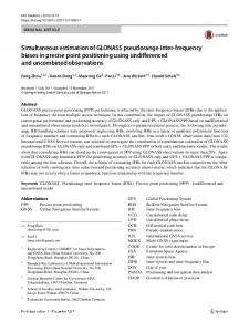
Figure 1. Imaging system model.
3. Modelling the imaging system We assume a simple imaging setup, where the camera views a reflectance target that is illuminated by a light source (figure 1). The light source produces illumination with a power spectrum I(λ). The spatial distribution of the light may not be isotropic. The light falling on a small area p of the reflectance target at time t is given by δp(t)I(λ) where δp(t) represents the radiant flux on p at time t. The reflectance target located at p at a particular time t has a reflectance function Tp(λ,t). The light received by the lens is determined by the product of these functions: δp(t)I(λ)Tp(λ,t). The lens aperture at time t applies a multiplier αp(t), also dependent on p because the effective aperture varies over the image field (due to vignetting). The colour filter within the camera (if a colour camera is being calibrated), in combination with the sensor response characteristics, introduces a wavelength-dependent filter function Fb,p(λ) for each colour band b. Thus, the expected linear sensor response is given by the effective sensor irradiance Sb,p(t) = αp(t) δp(t) ∫ Fb,p(λ) I(λ) Tp(λ,t) dλ.
(1)
Since I(λ) and Fb,p(λ) do not vary with time, let ρb,p(t) = ∫ Fb,p(λ) I(λ) Tp(λ,t) dλ. We then obtain sb,p(t) = αp(t) δp(t) ρb,p(t).
(2)
However, the camera responds non-linearly to the effective sensor irradiance. The actual camera response is cb,p(t) = gb,p(sb,p(t)) for some unknown nonlinear function gb,p. It is this function gb,p that we wish to estimate and invert to correct the camera’s radiometric response.
A suitable representation of the non-linear function gb,p can be obtained using an artificial neural network. Artificial neural networks are universal approximators [6] and can be used to model any unknown function provided that the network is sufficiently complex. Thus, we assume that the non-linear function gb,p is a neural network with unknown parameter vector θ. Omitting the subscripts b and p for simplicity, we obtain c(t) = g(α(t) δ(t) ρ(t), θ).
(3)
Given measurements of the camera response at N discrete times, we obtain N measurements of c(t) for each sensor element. However, if the system parameters represented by α(t), δ(t), and ρ(t) are changed for each sample time t then there are many more unknowns than measurements. In order to obtain information about the parameter vector θ, we must ensure that the number of different values of α(t), δ(t) and ρ(t) is less than N. A possible approach is to fix δ(t) = δ and to select α(t) and ρ(t) from discrete sets A = {α1, α2, …, αm} and R = {ρ1, ρ2, …, ρn} respectively. Provided that m+n+1 < N, there will be some data available to estimate the parameter vector θ. A possible experimental procedure is as follows. Set the camera to aperture α1 then pass the entire set of reflectance targets under the camera obtaining n measurements for each pixel. Change the aperture to α2 and again image all the reflectance targets. This procedure produces mn measurements for each pixel. Unfortunately, simultaneous estimation of A, R and θ based on measurements that vary the aperture and the reflectance target cannot determine the gamma factor of g. i.e., given c(t) = g(α(t) ρ(t) δ), there exists a family of solutions c(t) = hγ(α(t)γ ρ(t)γ δγ) where hγ(x) = g(x1/γ) and γ may be arbitrarily varied. (This is a straightforward generalisation of Grossberg and Nayar’s exponential ambiguity [4]). The family of solutions arises because the parameters that are being varied are combined by multiplication. In order to determine the gamma factor of g, we require additional, non-multiplicative constraint relationships. Of the three parameters that can be varied (aperture, irradiance and reflectance), irradiance is the most flexible – we cannot use more than one camera aperture at a time, and we can only use one reflectance target at a time in our inexpensive approach. However, using multiple light sources, we can create patterns of irradiance that incorporate additional constraint relationships. For example, using two light sources we can obtain four irradiance patterns. The two obvious patterns are δ1 where the first light is switched on, and δ2 where the second light is switched on. Two
additional patterns are δ3 = δ1+ δ2 where both lights are switched on and δ4 = 0 where both lights are switched off. In reality there is usually some ambient illumination δ0, so our equations become δ3 = δ1+ δ2 − δ0 and δ4 = δ0 yielding a single constraint relationship δ3 = δ1+ δ2 − δ4. This constraint relationship introduces an additive term into the equations for the camera response, overcoming the ambiguity with regard to the gamma factor. When multiple light sources are used in this manner, they should all have the same spectral distribution. In deriving equation 2 above, we assumed that I(λ) does not change over time so if we are using multiple lights in varying amounts, all the lights should have the same spectral distribution, including the ambient light. Alternatively, we could allow the light sources to have different spectral distributions if we required all the reflectance targets to have the same spectral characteristics except for a scaling factor, so that we could write Tp(λ,t) = τp(t) T(λ). However, our technique requires a large number of reflectance targets and it is easier to obtain the necessary diversity if we do not require a constant spectral distribution for the reflectance targets. In practice, we use the same type of lamp for all the light sources so that variations in the spectral distribution are minimal. We also use a darkened room so that the ambient illumination consists only of scatter from the light sources.
4. Data collection The basis of our technique is to fix the camera aperture and to vary the irradiance and reflectance. Four light sources are used, providing 16 irradiance patterns. The four light sources are of the same type but vary in irradiance because they are placed at different distances from the imaging area. Between 40 and 50 reflectance targets are used. Each reflectance target is imaged under each of the 16 irradiance patterns, yielding around N=700 measurements of the camera response for each pixel location. The light sources we use are low voltage halogen lamps connected to a DC power supply to ensure that the power output of each lamp is constant over time. Of course, the lamps cannot be switched on and off electrically as this would create temporal variations in intensity due to heating and cooling of the filament. Instead, shutters are used to control each light in a reproducible manner. However, a small amount of scattered light is present even when the lights are all shuttered off. This provides the ambient illumination allowed for in the model. The reflectance targets are uniformly coloured. We use samples of Pantone coloured paper in shades of
grey and various colours. The reflectance targets should represent the range from black (although an absolute black target is not available) through to white. The four light sources are set up at different distances for the reflectance target so that the irradiance values of the light sources are approximately related to each other by powers of two. Thus, if the most distant light source has a relative irradiance of 1, the other light sources have relative irradiances of 2, 4 and 8. Combinations of these light sources then provide all integer relative irradiance levels between 0 (all light shutters closed) and 15 (all light shutters open). The lens aperture of the camera and the distances to the light sources are chosen so that the most reflective targets will saturate the camera when illuminated with the greatest irradiance levels. If this is not done, there will be very little data available for the higher levels of sensor irradiance. In practice, we set up the imaging system so that a white reflectance target only just saturates the camera when exposed to the closest single light source. This ensures that less reflective targets also result in camera saturation at the higher irradiance levels provided by multiple light sources and thus sufficient data is collected for camera response levels just below saturation. In a simple set up, the light sources are physically separated so that they can be independently controlled by shutters. This means that the orientation of the light from each source is different as it reaches the reflectance target. The reflectance targets therefore must be uniformly flat in order that the relative irradiance levels of the different light sources remain the same for all reflectance targets. If the surface orientation varies for different reflectance targets, the changes in incidence angle of the illumination produce changes in the optical flux on the surface so that δ(t) is no longer independent of ρ(t). In some of our experiments, we observed unusually large data fitting errors that corresponded to a single reflectance target. Upon investigation, we found that the particular reflectance target had been bent due to handling and was no longer flat. The change in the surface orientation of the particular target, although not very large, was sufficient to disturb the relative irradiance levels from the different light sources and create the unusually large data fitting errors.
5. Artificial Neural Network Model We have already indicated that the unknown camera response function g can be modelled using an artificial neural network. In particular, a standard back propagation network with one input node, one output node, and several sigmoidal hidden nodes can be used
1 δ0 d1(t) d2(t) d3(t) d4(t)
δ1 δ2 δ3
+
δ4
δ(t) S
1
* r1(t) r2(t) r3(t) r4(t) ... rn(t)
ρ1 ρ2 ρ3 ρ4 ... ρn
1 +
ρ(t) δ(t)
S S S S
+ g(ρ(t) δ(t))
ρ(t)
Figure 2. Artificial neural network model.
to represent the function g. A direct shortcut link from the input to the output node is also used so that the network can more easily approximate near-linear functions. In fact, the entire equation 3 can be represented as a feedforward neural network, as shown in figure 2. In the diagram, nodes labelled ‘+’ are linear nodes calculating the weighted sum of their inputs. The labels on the connecting lines represent the weights. Nodes labelled ‘S’ are sigmoidal nodes – they calculate the weighted sum of their inputs, add a weighted bias and apply a sigmoidal activation function. The node labelled ‘*’ is a multiplier node – it multiplies its weighted input values together. The node labelled ‘1’ is a bias node. The inputs to the neural network d1(t), d2(t), d3(t) and d4(t) represent the states of the four light sources at each point in time. The input value is 1 if the light source is on, and 0 if the light source is off. The network weights δ1, δ2, δ3, and δ4, will be adapted by the network training to represent the relative irradiance values of the different light sources. Note that a separate neural network solution is obtained for each pixel location and each colour band of the camera, so differences in the spatial distributions of the light sources do not lead to errors in the modelling process. The node labelled δ(t) will calculate the irradiance at time t to within a scale factor. The inputs r1(t), r2(t), …, rn(t) represent the reflectance target in place at time t. Each input represents a separate reflectance target. The input value will be 1 corresponding to the reflectance target
6. Extracting the response function After training, the neural network contains a representation of the camera response function g. However, due to the arbitrary scaling and bias, the last portion of the neural network cannot be used directly as an estimate of g. Instead, we must extract the camera response function by operating the entire neural network within its trained range. For example, suppose that the first reflectance target is the most reflective (white) target. We set δ1= δ2= δ3= δ4= 1, representing the greatest irradiance
1.0 Linearised Response
that was in place; all other input values will be 0. The network weights ρ1, ρ2, …, ρn will be trained to represent the relative reflectance values of each reflectance target. The node labelled ρ(t) will calculate the reflectance of the target in place at time t to within a scale factor. The multiplier node calculates ρ(t) δ(t) to within a scale factor. Since the aperture is unchanged throughout the experiment, the estimation of α is subsumed within the calculation of ρ(t) δ(t). Also, vignetting does not introduce errors because a separate neural network solution is obtained for each pixel location. The network is trained using the camera response values from a single pixel as the desired network outputs. In practice, the entire network cannot be trained successfully from scratch because of its complexity. A successful approach is to first train the portion of the network up to and including the multiplier node, using the camera response values as the desired output of this portion of the network. Effectively, this training stage assumes that the camera response is linear. The actual nonlinearity produces a large fitting error at this stage. However, the trained portion of the network can then be used as the starting point for training the entire network. Even when the camera is highly non-linear because of the video gamma factor, the initial training produces estimates for δ1, …, δ4 and ρ1, …, ρn that are sufficiently close to the correct values to facilitate subsequent training of the entire network. In our preferred implementation, the input and bias weights for the sigmoidal hidden nodes (S in figure 2) are initially specified so that the nodes themselves represent a smooth piecewise linear approximation to the camera response function. I.e. the input weights are fixed so that the transition from 0.1 to 0.9 (for example) occurs within a sub-range of the input, and the bias weights are selected so that the different hidden node transition regions form overlapping subranges that cover the input range.
0.0 0
100 200 Camera Response
300
Figure 3. A typical linearisation function. possible. If we then set ρ2 = ρ3 = … = ρn= 0 and vary ρ1 from 0 to 1, the output will represent the modelled camera response under maximum irradiance to a target varying between zero reflectance (absolute black) and white. Because the white target saturates the camera under maximum irradiance, the neural network output will represent the behaviour of the camera over the entire range from absolute black to white saturation. The camera response function extracted by this means includes the saturated behaviour of the camera. However, saturated camera responses cannot be accurately converted to linear responses, so the useful range of camera response is limited. In our experiments, we found that the useful range of camera response was up to 70% of the maximum response. Beyond this point, the camera response curve changed rapidly as the camera became saturated. In fact, we found it better to discard data beyond 85% of the maximum response so that the neural network fitting is concentrated on the useful range of data. Using the technique that we have described, the camera response function can be estimated. It is then a simple matter to derive a lookup table that converts image data to linearised image data. By convention, the input to the lookup table is an integer pixel value on the range 0 to 255 and the output is a floating point linearised value. We compute the table so that an input of 178 (70% of 255) produces an output of 0.7 while an output of 0.0 is produced for all pixel values less than or equal to absolute black. Figure 3 shows a typical result for a colour CCD camera with gamma disabled. As we have presented it, the analysis produces a separate linearisation function for each pixel and for each colour band. In practice, we have found that the curves for different pixels are similar enough to
Deviation from linear
0.04
0.02
0.00
-0.02 0
100
200
300
Camera response
Figure 4. Non-linearity of two systems. warrant combining them together and using a single curve to represent the camera response for each colour band. However, if individual pixels exhibit sufficiently distinct behaviour, it is possible to derive separate linearisations for each camera pixel. This may require more data and improved neural network fitting techniques to achieve the required accuracy.
7. Experimental results
Difference from target value
We have experimentally tested this method of deriving a camera linearisation function. For our primary tests, we employed two completely separate systems composed of identical components – a JVC 3chip CCD video camera (KY-F55BE), Data Translation frame grabber DT3154 and PC. We calibrated each camera and frame grabber combination independently. Figure 4 displays the deviations of the two systems from linear response. The systems deviate from linear by up to 1.5% over the useful range while the two systems differ from each other by up to 1%. To test dependency of the results upon experimental
Deviation from linear
0.04
0.02
0.00
-0.02 0
procedure, we calibrated each system twice, using two independent sets of reflectance targets to derive two separate linearisation curves for each system. We found that the independent curves agreed with each other to within 0.2% maximum disparity (figure 5). To test agreement between the two systems, we used the linearised cameras to measure an independent collection of reflectance targets consisting of laboratory reflectance standards and ceramic tiles. The colour measurement was spatially averaged over each calibration target to reduce the effects of camera noise. These experiments showed an agreement in colour measurement between two independently calibrated cameras of 0.15% RMS, yielding a 95% confidence interval of ±0.003 (where 0 represents absolute black and 1 represents 100% reflectance). This is an excellent result for an 8-bit frame grabber and a camera with three bits of camera noise. Figure 6 shows the deviations of the two systems from the expected target reflectance values as a function of the target reflectance. The expected target reflectance values were measured using systems calibrated by our technique. This was necessary because of a lack of suitable independent calibration data. Firstly, the ceramic tiles were uncalibrated. Secondly, the available calibration data for the laboratory reflectance standards was based on hemispherical measurement whereas the camera systems measure only directional reflectance, introducing a detectable bias. As shown in figure 6, only one measurement exceeds a disparity of 0.3% from the expected value. To further explore the differences between the two systems, we performed crossover experiments in which the camera from each system was combined with the frame grabber from the other system. The linearisation curves derived from these crossover systems were very 0.002
0.000
-0.002
-0.004 0.0 100
200
300
0.2
0.4 0.6 Target reflectance
0.8
1.0
Camera response
Figure 5. Same system, repeat analysis.
Figure 6. Differences between systems.
close to the original curves of the system from which the camera was taken, demonstrating that most of the difference between the systems was contained in the camera and not the frame grabber. In a final practical experiment, we used the calibrated systems for biscuit colour inspection. The same biscuit samples were imaged by both systems. The agreement between the assessments of biscuit bake colour from the two systems exceeded the capability of human experts to make consistent assessments.
8. Discussion It is often assumed (e.g. [12]) that an image taken with no exposure to light represents the black-level response of the camera. We found that this assumption is not true for the equipment that we used. In particular, the combination of video camera and frame grabber produced a response to a fully black image that was brighter than the response to a black target in a well lit scene. Our specific experimental procedure overcame this issue by maintaining a constant background scene that provided a reference for the video capture system. The reflectance targets therefore occupied only a portion of the imaging area. In order for the background scene to provide a constant reference signal, we required a constant camera aperture. It was thus not possible to use aperture adjustment in our method. Newer digital cameras may not require a constant reference signal, in which case aperture variation may be used instead of reflectance target replacement during data collection (section 4). It will then be possible to characterise the camera response curve individually for each and every camera pixel. The analysis methods will remain the same. As far as we are aware, this is the first work to experimentally study the camera response curve for individual CCD camera pixels. The analysis that we have performed to date supports the commonly made assumption that the camera response curve is the same for all pixels. Nothing about the technique we have described requires that the sensor be a camera. We analysed data from many pixel locations and averaged the response curves together. However, the technique could equally be applied to a single light sensor such as a photoelectric cell. The only requirements for the technique are stable, spectrally matched light sources and a modulating technique such as reflectance target replacement, aperture adjustment or filters. Other authors have suggested alternative modelling techniques such as polynomial models [10] and basis functions derived from a database of camera response functions [5]. It would be interesting to explore how
these modelling techniques could be combined with the simultaneous estimation of illumination and reflectance.
9. Conclusion We have presented a practical method for the radiometric calibration of video cameras using multiple light sources and reflectance targets or aperture adjustment. A calibration accuracy of 0.2% disparity has been demonstrated using real images, a significant improvement on previous results. Colour measurements from independently calibrated systems agree to within 0.3%. Cameras calibrated by this method have been practically used for biscuit colour assessment.
10. References [1] H. Farid, “Blind Inverse Gamma Correction”, IEEE Trans. Image Processing, vol. 10, no. 10, 2001. [2] C. Grana, G. Pellacani, S. Seidenari and R. Cucchiara, “Color Calibration for a Dermatological Video Camera System”, Proc. Intl. Conf. Pattern Recognition, 2004. [3] M.D. Grossberg and S.K. Nayar, “What is the Space of Camera Response Functions?”, Proc. IEEE Conf. Computer Vision and Pattern Recognition, 2003. [4] M.D. Grossberg and S.K. Nayar, “Determining the Camera Response from Images: What is Knowable?”, IEEE Trans. Pattern Analysis and Machine Intelligence, vol. 25, no. 11, pp 1455-1467, 2003. [5] M.D. Grossberg and S.K. Nayar, “Modeling the Space of Camera Response Functions”, IEEE Trans. Pattern Analysis and Machine Intelligence, vol. 26, no. 10, 2004. [6] K. Hornik, M. Stinchcombe and H. White, “Multilayer Feedforward Networks Are Universal Approximators”, Neural Networks, vol. 2, 359-366, 1989 [7] S. Lin, J. Gu, S. Yamazaki and H.-Y. Shum, “Radiometric Calibration from a Single Image”, Proc. IEEE Conf. Computer Vision and Pattern Recognition, 2004. [8] C. Manders, C. Aimone and S. Mann, “Camera Response Function Recovery from Different Illuminations of Identical Subject Matter”, Proc. IEEE Intl. Conf. Image Processing, pp 2965-2968, 2004. [9] S. Mann and R. Picard, “Being ‘Undigital’ with Digital Cameras: Extending Dynamic Range by Combining Differently Exposed Pictures”, Proc. IST’s 48th Annual Conf., pp 422-428, 1995. [10] T. Mitsunaga and S.K. Nayar, “Radiometric Self Calibration”. Proc. IEEE Conf. Computer Vision and Pattern Recognition, 1999.
[11] T. RayChaudhuri, J. Yeh, L. Hamey, S. Sung and T. Westcott, “A connectionist approach to quality assessment of food products”, in Proc. Eighth Australian Joint Conference on Artificial Intelligence (X. Yao, ed.), pp. 435-441, 1995.
[14] J. Yeh, L. Hamey, C. Westcott and S. Sung, “Colour bake inspection system using hybrid artificial neural networks”, Proc. IEEE International Conference on Neural Networks, vol. 1, (Perth, Australia), pp. 37-42, 1995.
[12] K. Shafique and M. Shah, “Estimation of the Radiometric Response Functions of a Color Camera from Differently Illuminated Images”, Proc. IEEE Intl. Conf. Image Processing, pp 2339-2342, 2004.
11. Acknowledgements
[13] Y. Tsin, V. Ramesh and T. Kanade, “Statistical Calibration of CCD Imaging Process”, Proc. IEEE Intl. Conf. Computer Vision, pp 480-487, 2001.
This research was supported by the Cooperative Research Centre for International Food Manufacture and Packaging Science and Arnott's Biscuits Limited.