Simultaneous Extraction of Temporal, Spatial, and Spectral Information from Multi-Wavelength Lidar Data Charles E. Davidson Science and Technology Corp. 500 Edgewood Rd, Suite 205 Edgewood, MD 21040 410-436-2529
[email protected]
Avishai Ben-David Edgewood Chemical Biological Center, Aberdeen Proving Ground, MD 21010 410-436-6631
[email protected]
Abstract—Analysis of lidar data is generally done through parametric analysis where the lidar range dependent backscattering and extinction are deduced from the analytical lidar equation, and the range dependent concentration is deduced from the backscattering (or extinction). In previous work we have treated lidar measurements as a hyperspectral vector and applied traditional anomaly detection to determine (from one wavelength) the presence of a cloud of interest. Multiwavelength lidar data, however, is not a matrix (range-bytime), but instead is a tensor: a multidimensional n-way array (range-by-time-by-wavelength). Matrix analysis techniques such as anomaly detection will not extract all the information available within this array. This work describes the use of n-way analysis techniques to simultaneously extract temporal, spatial, and spectral information from multi-wavelength lidar data.12
a multi-wavelength lidar system can be used to infer information such as chemical identity, concentration, and aerosol particle size distribution as a function of range. Usually analysis of lidar data is accomplished by solving the analytical lidar equation[2], of which there are many methods. In most field experiments, however, a vast amount of data is collected within seconds, and evaluating each data set prior to a more detailed and time-consuming analysis is often of interest when immediate information such as the whereabouts (time & location) and a rough estimate of cloud’s spectral characteristics of the cloud within the lidar field is of view is sought, e.g., real time remote sensing applications). Previously[4], we attempted to characterize data from a multi-wavelength IR lidar system[5] that repeatedly measured the backscatter along a single line-of-sight for 19 wavelengths, for the purpose of detecting aerosol clouds. These data were naturally arranged as a 3-dimensional (3D) array giving the return intensity as a function of range, time, and wavelength: X(r,t,λ). We drew from common linear algebra (matrix) techniques to answer the question, “is a target cloud of interest present between ranges R1 and R2?” An algorithm was developed to compress each range vector to a scalar quantity, or score. If the score exceeded a threshold for the return at time ti, this indicated the presence of a cloud somewhere between R1 and R2. Although useful, the technique could only be applied to one wavelength at a time, therefore ignoring relationships among wavelengths that might improve performance.
TABLE OF CONTENTS 1. INTRODUCTION ......................................................1 2. N-WAY ANALYSIS .................................................2 3. THE HOSVD .........................................................3 4. METHOD ................................................................3 5. RESULTS ................................................................5 6. CONCLUSION .........................................................7 REFERENCES .............................................................8 BIOGRAPHY ...............................................................9
1. INTRODUCTION A lidar system emits a laser pulse and measures the intensity of light returned to the source, and is commonly used in atmospheric studies, range-finding, and other applications[13] . In the infrared (IR), the intensity of received light (backscatter) depends on the scattering and extinction properties of the medium as a function of range, and so the lidar backscatter can be used to deduce these properties. Since the wavelength dependence of these properties is related to the physical and chemical content of the medium,
In this work, we draw from a set of related fields (n-way analysis, multilinear algebra, tensors) that allows algebraic manipulation of multidimensional arrays. Using these techniques, a method is developed to characterize the 3D lidar data that incorporates range, time, and wavelength relationships simultaneously. This paper is organized as follows. In section 2, a brief summary of n-way analysis is presented, including terminology and notation. In section 3, a method for extracting sources of variation from multidimensional arrays, the higher-order singular value decomposition
1
1
1-4244-0525-4/07/$20.00 ©2007 IEEE IEEEAC paper #1183, Version 5, Updated February 5, 2007
2
1
(HOSVD), is reviewed. In section 4, the method used to characterize the multi-wavelength lidar data is described. In section 5 the method is applied to actual lidar field data. Conclusions are presented in section 6.
wavelength matrices for the various times; or a series of time-by-wavelength matrices at the various ranges. These types of abstractions about multidimensional arrays are useful in developing generalizations of linear algebraic techniques to higher-order arrays. Unfolding Higher-Order Arrays
2. N-WAY ANALYSIS
One way in which n-way analysis enables the manipulation of higher-order arrays is by finding an appropriate matrix or vector representation of the arrays such that common linear algebra methods will accomplish the desired computation. Here, the term “unfolding” will refer to the representation of a multidimensional array as an entity with fewer modes.
Scientists and engineers are comfortable dealing with matrices or tables of numbers. These types of 2dimensional (2D) data arrays contain information about the relationship between one variable and another. Various manipulations and geometric interpretations of these matrices are defined and well-understood in the field of linear algebra. Extending these arrays to 3 dimensions or more can be a natural way to describe data that are a function of multiple variables. Unfortunately, equivalent algebraic operations and geometric interpretations are not always as straight-forward or as well-known as for the matrix case, and analysis of these arrays is usually accomplished by ignoring one (or more) dimensions altogether. However, methods for manipulating these higher-dimensional arrays do exist in the fields of n-way analysis, multilinear algebra, and tensors.
Unfolding an array such that all dimensions but one are combined into a single mode is referred to as the “mode-n unfolding” of the array, and it produces a matrix containing all the vectors defined by the nth mode (also called the mode-n vectors). The nth dimension of the array becomes the first index of the matrix, and the second index refers to all the other modes interleaved. For example, the mode-3 unfolding of the lidar array X(r,t,λ) is a λ-by-rt matrix whose columns are all the spectra in the data set for all combinations of range and time; it is said to contain all the mode-3 vectors of X.
N-way analysis has its roots in many disciplines, being developed over the past 40 years or more[6-8]. Because of this, terminology, notation, and conventions are highly variable. It is too early to tell if attempts at new notation[9] or standard terminology[10] will catch on; in general authors pick and choose as they will. This paper is no exception, but in order to mitigate any possible confusion, terminology and notation are explicitly defined in this section. The reader is encouraged to refer to the literature[6-11] for a more detailed presentation of n-way concepts.
Notation In this paper, lower-case italic letters (a, b,…) are scalars, bold lower-case letters (a, b,…) are vectors, bold capital letters (A, B,…) are matrices, and higher-order arrays are capital script-style letters (A, B,…). Subscripts in square brackets specify the size of each dimension of the array, e.g., a 3D array of size 3-by-3-by-2 is specified as A[3,3,2]. Parenthetical subscripts will be used when it is convenient to refer to an array that is unfolded into matrix form. For instance, X(3) refers to the mode-3 unfolding of the lidar array described above.
Higher-Order Arrays The “order” of an array is the number of indices (also called “modes”, “dimensions”, or “ways”) necessary to refer to any element in the array3. A scalar entity is order 0, as it needs no indices or modes to refer to its value; a vector is an array of order 1, as one index or mode can refer to all its values. A matrix is a 2D array because it has two modes: a row index and a column index, and can be thought of as a table with scalar-valued elements. The lidar data array has row and column indices referring to range-bin and time-bin, respectively, as well as a third mode that refers to the wavelength. It can be thought of as a table (range-by-time) whose elements are spectral vectors. Or, it can be thought of as a series of matrices (slices of the 3D array) stacked behind (or beside or on top of) one another. For the lidar data, these slices could be: a series of range-by-time matrices at the various wavelengths; a series of range-by-
An alternate notation will also be used to specify and refer to n-way arrays. The notation X(r,t,λ) will be used to specify a 3-way array whose modes are the variables r, t, and λ, respectively. Referring to X as a function of a subset of those variables should be understood to signify that unspecified modes take all of their values, while the specified variables are iterated through a range of values. For example, X(λi) would refer to the ith r-by-t matrix in the array X; x(tj,λi) would refer to the range vector in X for the ith value of λ and the jth value of t; x(rk,tj,λi) would refer to the kth element for range, the jth element for time, and the ith wavelength element (i.e., a single value). Multiplying Higher-Order Arrays
2
There are many ways of defining multiplication involving higher-order arrays. Several definitions that are of special
3
In the tensor community “rank” is commonly used for the number of indices of an array. We discourage this use because of the possible confusion with the matrix rank from linear algebra.
2
interest are the array outer product (or tensor product) and the n-mode product.
3. THE HOSVD The singular value decomposition (SVD) is defined in Eq. 3, where A is an m-by-n matrix such that U and V are the orthonormal matrices of eigenvectors of AAT and ATA, respectively; S is the diagonal matrix of singular values, and p is the rank of A, where “rank” denotes the number of linearly independent vectors in a matrix (i.e., the linear algebra definition of rank). If the data A is real, the first eigenvector of U is the direction in ℜm from the origin to the mean of the data, the remaining eigenvectors are ordered in decreasing explained variance (i.e., the singular values in S are arranged in decreasing order).
Recall that the vector outer product between m-by-1 vector a and n-by-1 vector b is an m-by-n matrix
C = ab T = a D b containing all possible multiplications
of an element in a with one in b (superscript T denotes the transpose operation). In linear algebra, no similar operation is defined for matrices. The array outer product is a generalization of the vector outer product that finds all possible multiplications between an element in A and one in B regardless of whether A and B are vectors, matrices, or higher-order arrays. If A is order K with dimension sizes [i1, i2, …, iK] and B is order L with dimension sizes [j1, j2, …, jL], then the product C is the (K+L)-dimensional array given by
C = ci1i2 ...ik j1 j2 ... jL = ai1i2 ...ik b j1 j2 ... jL = A D B
p
A = USV T = ∑ si u i D v i
(1)
Just as the SVD decomposes a matrix into a sum of outer products between a row vector and a column vector, the HOSVD[12] decomposes an n-way array into a sum of outer products of mode-n vectors. The HOSVD is calculated by first performing SVD on each mode-n unfolding of a higher-order array A to produce n separate U matrices; the notation U(n) refers to the U matrix found from the SVD of the 2D matrix A(n). Then, the core tensor S (which has the same order as A and acts as a set of mixing coefficients for the linear combination of the vectors in the U(n) matrices) is found using Eq. 4. The decomposition of the 3-way array A
The array outer product between m-by-1 vector a and n-by1 vector b is an array of size [m 1 n 1]. Since explicit singleton dimensions may be ignored, the result is an m-byn matrix. Note that the outer product of 3 vectors will produce a 3D array. The array outer product plays an important role in the HOSVD. The n-mode product[12] is an extension of matrix multiplication that allows a higher-order array to be multiplied by a matrix. Recall that in the multiplication AB, all dot products between a row (or mode-2) vector in A and a column (or mode-1) vector in B are computed. If a higher-order array A is involved in the multiplication, there is ambiguity over which mode in A will participate. For instance, should row vectors, column vectors, or vectors defined by some other mode be dotted with the vectors in B? The n-mode product introduces the subscripted “×n” symbol to specify the mode in A that participates in the dot product. In contrast to matrix multiplication, in the n-mode product it is understood that row (mode-2) vectors of B participate in the multiplication. The n-mode product operation is given in Eq. 2, and uses the convention that the surviving dimension in B (index j) replaces the nth dimension of A (index in) in C.
C = ci1i2 ... j ...iK = ∑ ai1i2 ...in ...iK b jin = A × n B
(3)
i =1
(n )
using HOSVD is given in Eq. 5, where u i column vector of matrix U
(n)
is the ith
and pi is the rank of A(n). T
T
S = A ×1 U (1) × 2 U ( 2 ) × 3 U ( 3)
T
(4)
A = S ×1 U (1) × 2 U ( 2) × 3 U (3) p1
p2
p3
= ∑∑∑ u i(1) D u (j2 ) D u (k3) sijk
(5)
i =1 j =1 k =1
4. METHOD The analysis method presented here is a four-step process. First, the data undergo a preprocessing step to help remove unwanted signatures. Second, the HOSVD is used to identify range, time, and wavelength profiles characteristic of the signal of interest. Third, the profiles are correlated to the lidar data to produce detection scores. Finally, a statistical analysis of the detection scores yields a set of binary detection maps.
(2)
in
The n-mode product can be used, for example, to calculate the dot product between some spectral vector y (λ-by-1) and all the spectral vectors in the lidar data X(r,t,λ): C = X ×3 y T . The result, C, is an r-by-t matrix giving the correlation to y at every range and time.
3
Step 1: Preprocessing
too many eigenvectors are used), distortions can be introduced into the signal of interest. Therefore we chose to include only one eigenvector in the OSP operator.
In lidar data, it is a common objective to remove unwanted shape or signatures in the measured signal in order to better detect the signal of interest. Unwanted shape or signatures could include the inverse range squared dependence of the backscatter, the presence of ambient aerosols, and hardware noise. In previous work with lidar data[4] we used an orthogonal subspace projection (OSP)[13,14] operator to remove such signatures, and a similar method is applied here.
Step 2: HOSVD After OSP filtering, we assume that the largest source of variation in the data for each mode corresponds to the signal of interest. Therefore, the HOSVD was applied and the first eigenvector for each mode was retained as the characteristic profile of the signal for that mode. These vectors give the direction of largest variation in relation to the origin (defined as the center of the H0 condition due to the OSP operation) in range, time, and wavelength spaces, and are referred to as the range profile U(1), temporal profile U(2), and spectral profile U(3), respectively.
In OSP, a projection operator is found that projects the original data onto a subspace that is perpendicular to the unwanted signatures, thereby annihilating them. Unwanted signatures are usually identified from the first few vectors of the eigenvector matrix U from the SVD of background data: a subset of data thought to be clear of “important” signal. The projection operator is defined in Eq. 6, where I is the identity matrix and superscript -1 denotes the matrix inverse operation .
(
P ⊥ = I − U UT U
)
−1
UT
Step 3: Detection Scores The correlation (dot product) of the data to each of the mode profiles is calculated using the n-mode product: T C ( n ) = Xˆ × n U ( n )
(6)
Each 2D C(n) matrix gives a similarity score for the lidar data in relation to the profile for the nth mode as a function of the other two modes. For instance, C(3) is an r-by-t matrix giving the spectral similarity for all combinations of range and time. Together, the three C(n) matrices represent all relationships between range, time, and wavelength. The C(n) matrices will be referred to as the scores or score matrices.
In our lidar data, measurement began about a minute prior to aerosol release. This gave a population of returns for each wavelength in which only atmospheric ambient aerosols were in the field of view. This period of time is used to define the background or H0 (null) condition. An ⊥
OSP operator ( Pλk ) is found from the background range vectors X(λi) at each wavelength. Each r-by-r matrix represents a projection from the original measurement space to a subspace perpendicular to the first vector of U. The OSP operators are applied to the data according to Eq. 7.
Since the HOSVD finds eigenvectors with an indeterminacy of multiplication by -1, there is no guarantee that the polarity of the n-mode profiles will match the polarity of the corresponding signal in the data. To rectify this, the maximum element of the absolute value of each C(n) is located. If the sign of this element is positive, the n-mode profile has the correct polarity. Otherwise, U(n) and therefore C(n) [Eq. (8)] are both multiplied by negative one to correct the polarity.
The filtered lidar data array, Xˆ , was used in all further processing.
ˆ ( λ ) = P ⊥ X( λ ) X k λk k
(8)
(7)
This orthogonal projection process serves to adaptively remove the 1/r2 dependence of the signal captured by the first eigenvector of U, and may also remove contribution from ambient aerosols4. This step also sets the origin of the data space to be the center of the H0 condition, so that the directions found in the HOSVD will be in relation to the background, and therefore more meaningful for identifying signals of interest.
Step 4: Statistical Analysis Score matrices C(n) are used to infer the statistical properties of the H0 condition. A one-sided hypothesis is assumed, and so correlation values less than zero are attributed solely to the H0 case (i.e., signal of interest is absent) and used to estimate the probability distribution function (PDF) of H0 on the interval (− ∞, 0 ) . The PDF of H0 is further assumed to be zero-centered and symmetric. The corresponding cumulative distribution function is used to find a threshold with a desired false alarm rate; score values greater than the threshold correspond to detection. This produces binary yes/no detection maps for each score matrix (range vs wavelength, time vs wavelength, and range vs time). If any of the assumptions about the nature of the H0 distribution
Including a larger number of U vectors into the OSP filter was considered. This would remove a larger portion of variance characteristic of the background from the data. However, if the orthogonal subspace is too restrictive (i.e., 4 4
An alternate method of removing the inverse range squared dependence is range correction, which multiplies the lidar return by r2. This procedure, however, amplifies noise and is incapable of removing other interferences.
4
are invalid, then the actual observed false alarm rate will be different than the expected false alarm rate.
a function of range) is evident in this image. It should be noted that calculating the noise in this way will include some variation from the scene (i.e., ambient atmospheric aerosols) in the estimate, and therefore overestimates the instrument noise.
5. RESULTS The frequency agile CO2 lidar (FAL) system[5] was set 880 m away from the aerosol cloud release point at Dugway Proving Ground, UT, in April of 2006. The FAL uses a CO2 transverse excited atmospheric (TEA) laser (2.5 mrad beam divergence) with a wavelength range of 9.3-10.7 microns at an output energy of 150-220 mJ per pulse, and is coaxially aligned with a 14-inch receive telescope (3 mrad field of view) with a liquid-nitrogen cooled HgCdTe (mercury cadmium telluride, also abbreviated as MCT) detector. One “burst” consists of nineteen consecutive laser pulses that span the entire wavelength range. Although the 19 pulses are not simultaneous in time, they occur quickly enough in relation to the expected time-scale of changes within the scene that they can be considered virtually simultaneous (the pulse rate is 200 Hz). If this assumption is faulty then some distortions will be present in the spectral response. At a 1 Hz burst repetition rate, 1 transmit and receive pulse is recorded for all wavelengths every second. To remove the effect of the long lidar transmit pulses (as much as 2 μs) and the limited bandwidth used in the receiver’s detector and amplifier, the lidar returns are normalized5 by the transmit pulse area prior to analysis.
70 250
60 50 40
150 30 100
20
50
10
Mean S/N
Range Bin
200
0 200
400 600 Time Bin
800
1000
Figure 1: S/N of the data prior to OSP filtering. The average S/N across wavelengths after OSP filtering is shown in Fig. 2. While the 1/r2 dependence has been removed, there is also quite a bit of variation in the S/N image from range bins 1 to 125. This is due to the high level of variation in the location of where the divergence of the transmitted beam becomes completely within the fieldof-view of the receiver. In this test, the tunnel begins at a point 880 m from the lidar system (range bin 183), and so the remainder of the analysis has been limited6 to range-bins 150 to 281 (720-1349 m), where the upper range limit (1349 m) was chosen to be sure that a hard target in the field of view at 1.6 km was not included in the data.
Measurements of a Pantoea agglomerans (formally known as Erwinia herbicola or EH) aerosol cloud resulted in a relatively high signal-to-noise ratio (S/N). The standard deviation of each range-bin for each wavelength over the first 100 returns (100 seconds) in time was used to estimate the noise. The average S/N over all wavelengths for the raw data is displayed in Fig. 1. The cloud (upper portion of image) and 1/r2 dependence of the signal (gradual change as 5
5
The atmospheric backscattering signal measured by the FAL at time t’ (where t’ is time of flight of a transmitted photon) is interpreted as if it were from a backscattering event at a range r = ct ' / 2 (where c is the speed of light). However, the transmit pulse has some finite width Δt, and so the backscattered radiation observed at time t’ is actually due to a series of ranges from c (t '− Δt ) / 2 to ct ' / 2 . For each of these ranges the
5
backscattering intensity is reduced by the inverse range squared and the atmospheric transmission back to the receiver. For the FAL (a CO2 laser operating in the 9-12 μm window) the transmitted lidar pulses exhibit
6
It is important to note that one could have chosen to limit the range prior to the OSP preprocessing. However, this results in poorer detection performance. This suggests, possibly, that the strong magnitude of the shape of the 1/r2 dependence helps to set the direction of the first eigenvector. Because the 1/r2 shape is relatively small when the range vectors are subsetted to longer ranges, the background range vectors are very close to the origin, meaning that the expected value of the background is close to the zero-vector. We theorize that since the first eigenvector of the data is the direction from the origin to the mean of the data, and the mean of the data is so close to the origin, any error in estimating the true population mean would correspond to a large variation in direction. Another possible explanation is that as the mean of the data approaches zero, second order information may begin to influence the direction of the first eigenvector, making it less effective at annihilating the desired shape. Regardless of the reason, performing OSP on the full range vectors and then subsetting the range is more effective.
complex (i.e., non-rectangular) temporal shape[15,16] and therefore the lidar return signal can be described as a convolution between the transmitted temporal pulse shape and a lidar backscattered signal for an infinitesimally short transmitted lidar pulse ( Δt → 0 ). In order to avoid a full deconvolution process[16] to account for the finite electronic bandwidth of the lidar receiver, the lidar transmitted pulse temporal shape, and the width of the cloud (~120 m), we normalize the lidar return signal with an area of the transmitted lidar pulse that is computed within ±120 m of the transmitted temporal peak location. This normalization process is a substitute for the lengthy deconvolution process, where we account for most of the transmitted photons that contribute to the return from a range resolution (i.e., the cloud) cΔt / 2 = 120 m .
5
Range Profile
70
250
60 50 40
150
30 100
Mean S/N
Range Bin
200
160
180
200 220 Range Bin
240
260
280
Temporal Profile
20 50
10 0 200
400
600
800
200
1000
Time Bin
400
600 Time Bin
800
1000
Spectral Profile
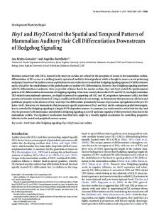
Figure 2: S/N after OSP filtering. The mode profiles from the HOSVD are shown in Figure 3. They represent the directions that explain differences between the H0 condition and the rest of the data in the hyperdimensional spaces defined by range, time, and wavelength. The range and time profiles track cloud strength as a function of range and time, respectively; the spectral profile shows the sensitivity of each wavelength to the presence of the cloud.
5
10 Wavelength Bin
15
Figure 3: Mode profiles U(n). These profiles represent the directions that explain differences between the H0 condition and the rest of the data in the range, temporal, and spectral hyperdimensional spaces. Since only direction is important the y-axis is arbitrary, and thus omitted.
From these profiles one can observe that the cloud is detected beginning at range bin 190 (912 m) and at time bins 190 to 870 (the time span of the cloud release within the lidar’s field of view). This is consistent with the ground-truth collected for the test (we note that 912 m places the cloud dissemination point within the tunnel, and field notes indicate the release began at time-bin 189). To interpret the spectral profile, one may compare to library spectra for identification purposes. However, this is a nontrivial step as any accurate comparison requires a radiometric model of the scene in order to make the library spectrum more realistic. The spectral shape seen here is commonly observed in FAL data: the dip in the spectral profile at wavelength-bin 13 corresponds to the 10R20 line of the CO2 laser where there is strong absorption by water[17].
The three score matrices C(n) are shown in Fig. 4, and give the similarity of each vector in the lidar data to each profile. The top image is of the range correlation map C(1), where similarity to the range profile is shown as a function of wavelength-bin and time-bin. The middle image is of the temporal correlation map C(2), where the similarity to the temporal profile is given as a function of wavelength and range-bins. The spectral correlation map or C(3) (bottom) gives the similarity of the lidar data to the spectral profile as a function of range and time bins. These score matrices give additional information about the aerosol cloud than is contained in the n-mode profiles. Not only are the range, time, and wavelength behaviors evident, but their behavior in relation to the other modes is also seen. This helps bolster the confidence in the results, i.e., different indications for the same results are given simultaneously using this method. For instance, looking at the range correlation map in Fig. 4 (top), it can be seen that all wavelengths result in similar range correlation results within time-bins ~200 to ~900, increasing the confidence of the temporal behavior of the cloud. From Fig. 4 (middle), the presence of a cloud between range-bins ~200 and ~250 is strongly indicated due to the fact that each wavelength reflects a similar anomaly in time.
6
0.2
5 200
400 600 Time Bin
800
0
1000
Wavelength Bin
10
Temporal Correlation 10 5 150
200 Range Bin
250
Correlation
0.8 0.6 0.4 0.2 0
15
Wavelength Bin
Wavelength Bin
0.4
15
Correlation
Wavelength Bin
Range Correlation
200
0.1
150
0
800
1000
Range Bin
Range Bin
0.2
Correlation
250
400 600 Time Bin
Figure 4: Score matrices C(n). These images show the correlation of the data to the range, temporal, and spectral profiles, respectively.
) ( )
T T C ( 2 ) = Xˆ ×1 U (1) ×1 Xˆ × 3 U ( 3) (1) T
( 3)
C
=C C
T ( 3) T
(1)
10 5 200
400
600 Time Bin
800
1000
Temporal Detection 15 10 5 160
180
200 220 Range Bin
240
260
280
250 200 150
200
400
600 Time Bin
800
1000
Figure 5: Score matrices C(n) thresholded at a 0.01 false alarm rate. Red pixels correspond to a detection: a location where the scores are greater than the threshold, and thus the cloud is presumed to be within the field of view. White represents no detection.
We observed for this data that the dot product of any two score matrices gives the third (to within machine precision). This equivalence (for calculating C(2)) is given by
( = (C
15
Spectral Detection
Spectral Correlation
200
Range Detection
Of the three detection maps in Fig. 5, the third (bottom) is perhaps the most useful since it gives the similarity to a spectral profile as a function of both range and time. In other words, the spatial and temporal extent of the cloud is shown simultaneously. For this data, it may also be argued to be the “best” of the three maps. The spectral response is reduced to a scalar value in this map, and so the correlations between wavelengths should contribute to a higher “confidence” that the physical presence of the cloud (in space and time) was detected correctly. The third map would also be the most useful in situations where multiple clouds are observed, as the similarity to different spectral profiles could be simultaneously displayed in different colors.
) (9)
A full mathematical derivation of this equivalence is not presented here, but it can be rationalized by noting that for any set of two score matrices, one mode serves as the independent variable for each of the other modes, and thus the set of score matrices implicitly contains information needed for the translation of variables. For example, since C(1) gives the wavelength response as a function of time, and C(3) gives range as a function of time, the dependence of wavelength on range (or C(2)) is contained therein.
6. CONCLUSION A data analysis method using techniques from n-way analysis has been developed and applied to multiwavelength lidar data. This method uses the higher-order SVD in order to extract characteristic profiles in range, time, and wavelength that relate to the signal of interest. An orthogonal subspace projection step prior to the HOSVD increases the likelihood that the most significant eigenvectors (mode profiles) from the HOSVD correspond to the desired signal. The profiles give valuable information about the behavior of the cloud in terms of where it was
The thresholded detection maps (at a 0.01 false alarm rate) are shown in Fig. 5. Values that are above the threshold are shown in red and correspond to the detection of the presence of the cloud within the lidar field of view. White pixels are below the threshold and indicate no detection. The PDF assumptions made in determining the threshold seem to be validated: empirical inspection yields about 1 false alarm per 100 pixels.
7
located, when it was observed, and which wavelengths responded to the presence of the cloud. By correlating the data with each mode-profile, the behavior of the data as a function of the two other modes can be found in the score matrices. Using these score matrices, detection maps giving the behavior of the cloud with respect to range vs. time (spectral detection), range vs. wavelength (temporal detection), and time vs. wavelength (range detection) were found at a false alarm rate of 1% (the detection probability remained unknown due to a lack of exact ground-truth information). These types of detection maps could be invaluable in cloud tracking, detection, and decontamination applications.
REFERENCES [1] W. B. Grant, “ Lidar for atmospheric and hydrospheric studies,” in Tunable Laser Applications, F. J. Durate, ed. (Marcel Dekker, New York 1995), pp. 213-305 [2] R. M. Measures, Laser Remote Sensing : Fundamentals and Applications, Wiley, New York (1984) [3] R. M. Measures, Laser Remote Chemical Analysis, Wiley, New York (1988) [4] A. Ben-David, C. Davidson, R. Vanderbeek, “Lidar detection algorithm based on hyperspectral anomaly detection,” 2006 International Laser Radar Conference proceedings, Jul. 24-28, 2006.
The method is very general, and is amenable to data with an arbitrary number of modes. For instance, if the FAL system measured the backscattered radiation at various polarizations for each wavelength, the added mode would result in a 4D data array, the HOSVD would pull out four profiles, and our method would be applied in the same way. There would be four detection maps, each a function of three variables. While the method was applied here to data containing a single cloud, it could be used to analyze more complicated data. For instance, if more than one cloud were present in the scene, more than one significant profile for each mode could be extracted. This would result in a separate set of detection maps for each cloud, which could enable independent tracking of each with respect to behavior in time, range, and spectral response.
[5]
A. Ben-David, “Backscattering measurements of atmospheric aerosols at CO2 laser wavelengths: implications of aerosol spectral structure on differential absorption lidar retrieval of molecular species”, Appl. Opt. 38, 2616-2624, 1999.
[6] L. R. Tucker, “Some mathematical notes on three-mode factor analysis,” Psychometrica 31, 279-311, 1966. [7] R. A. Harshman, “Foundations of the PARAFAC procedure: models and conditions for an explanatory multi-mode factor analysis,” UCLA Working Papers in Phonetics 16, 1-84, 1970.
Another advantage of this method is that it is data driven. No prior knowledge of the spectral shape or cloud location is needed in order to detect. The only requirement is to obtain background measurements when the lidar field of view is known to be clear of the aerosol cloud (H0 condition).
[8] J. D. Carroll and J. J. Chang, “Analysis of individual differences in multidimensional scaling via an N-way generalization of ‘Eckart-Young’ decomposition,” Psychometrika 35, 283-319, 1970. [9] R. A. Harshman, “An index formalism that generalizes the capabilities of matrix notation and algebra to n-way analysis,” J. Chemometrics 15, 689-714, 2001.
Future work at incorporating this method with a physical model may lead to improved estimates of concentration, particle size, and other physical parameters characterizing the aerosol cloud.
[10] H. A. L. Kiers, “Towards a standardized notation and terminology in multiway analysis,” J. Chemometrics 14, 105-122, 2000. [11] R. A. Harshman and S. Hong, “’Stretch’ vs ‘slice’ methods for representing three-way structure via matrix notation,” J. Chemometrics 16, 198-205, 2002. [12] L. De Lathauwer, B. De Moor, J. Vandewalle, “a multilinear singular value decomposition,” SIAM J. Matrix Anal. Appl. 21(4), 1253-1278, 2000. [13] J. Harsanyi and C-I Chang, Hyperspectral image classification and dimensionality reduction: an orthogonal subspace projection approach, IEEE Trans. Geocsi. Rem. Sens., Vol. 32, 779-785, 1994. 8
[14] L. L. Scharf, Statistical Signal Processing, Detection, Estimation and Time Series Analysis, Addison-Wesley, New York, New York, 1991. [15] A. Ben-David, “Optimal Bandwidth for Topographical DIAL Detection,” Appl. Opt. 35, 1531-1536, 1996. [16] A. Ben-David, “Mueller matrix for atmospheric aerosols at CO2 wavelengths from backscattering polarized lidar measurements,” J. Geophys. Res. 103, 26041-26050 1998. [17] A. Ben-David, Temperature dependence of water vapor absorption coefficients for CO2 differential absorption lidars, Appl. Opt., Vol. 32, 7479-7483, 1993
BIOGRAPHY Charlie Davidson earned his Ph.D. from Clarkson University researching methods for the analysis of chemical data, a subset of chemistry commonly called chemometrics. He has designed algorithms and software for clustering, pattern recognition, and classification of multivariate data with an emphasis on machine learning. Since joining STC he has focused on signal processing, algorithm development, and analysis of passive and active remote sensing data, as well as modeling and simulation of remote sensors and their physical environment. Avishai Ben-David is a research physicist in the U.S Army Edgewood Chemical Biological Center. He received his Ph.D. in Atmospheric Physics from the University of Arizona, Tucson in 1986. He has been active in theoretical and experimental research of passive (FTIR) and active (lidar) remote sensing for the past 20 years. His research interests include hyperspectral algorithms, radiative transfer in the atmosphere (aerosols scattering, absorption, thermal emission and polarization) and signal processing methods. He is involved in developing passive infrared remote sensing sensors and the evaluation of new technologies.
9