University of Wollongong
Research Online Faculty of Informatics - Papers
Faculty of Informatics
2005
Simultaneous Map Estimation of Inhomogeneity and Segmentation of Brain Tissues from MR Images W. Li University of Wollongong,
[email protected]
C. deSilver University of Wollongong
Y. Attikiouzel Murdoch University
Publication Details This paper originally appeared as: Li, W, deSilver, C and Atttikiouzel, Y, Simultaneous Map Estimation of Inhomogeneity and Segmentation of Brain Tissues from MR Images, IEEE International Conference on Image Processing, 11-14 September 2005, vol 2, 1234-1237. Copyright IEEE 2005.
Research Online is the open access institutional repository for the University of Wollongong. For further information contact Manager Repository Services:
[email protected].
Simultaneous Map Estimation of Inhomogeneity and Segmentation of Brain Tissues from MR Images Abstract
Intrascan and interscan intensity inhomogeneities have been identified as a common source of making many advanced segmentation techniques fail to produce satisfactory results in separating brains tissues from multispectral magnetic resonance (MR) images. A common solution is to correct the inhomogeneity before applying the segmentation techniques. This paper presents a method that is able to achieve simultaneous semi-supervised MAP (maximum a-posterior probability) estimation of the inhomogeneity field and segmentation of brain tissues, where the inhomogeneity is parameterized. Our method can incorporate any available incomplete training data and their contribution can be controlled in a flexible manner and therefore the segmentation of the brain tissues can be optimised. Experiments on both simulated and real MR images have demonstrated that the proposed method estimated the inhomogeneity field accurately and improved the segmentation. Publication Details
This paper originally appeared as: Li, W, deSilver, C and Atttikiouzel, Y, Simultaneous Map Estimation of Inhomogeneity and Segmentation of Brain Tissues from MR Images, IEEE International Conference on Image Processing, 11-14 September 2005, vol 2, 1234-1237. Copyright IEEE 2005.
This conference paper is available at Research Online: http://ro.uow.edu.au/infopapers/196
SIMULTANEOUS MAP ESTIMATION OF INHOMOGENEITY AND SEGMENTATION OF BRAIN TISSUES FROM MR IMAGES Wanqing Li, Chris deSilver*, Yianni Attikiouzel* School of Information Technology and Computer Science, University of Wollongong, Australia *Division of Science and Engineering Murdoch University, Australia ABSTRACT Intrascan and interscan intensity inhomogeneities have been identified as a common source of making many advanced segmentation techniques fail to produce satisfactory results in separating brains tissues from multi-spectral magnetic resonance (MR) images. A common solution is to correct the inhomogeneity before applying the segmentation techniques. This paper presents a method that is able to achieve simultaneous semi-supervised MAP (maximum a-posterior probability) estimation of the inhomogeneity field and segmentation of brain tissues, where the inhomogeneity is parameterized. Our method can incorporate any available incomplete training data and their contribution can be controlled in a flexible manner and therefore the segmentation of the brain tissues can be optimised. Experiments on both simulated and real MR images have demonstrated that the proposed method estimated the inhomogeneity field accurately and improved the segmentation. 1. INTRODUCTION Segmentation of Magnetic Resonance (MR) images is a process of delineating regions representing different types of tissues and/or lesions. In general, the following sources of information may be used in this process: • for each pixel (or voxel) an observation which may contain a vector of values, usually intensities, to characterise it, • a known tendency of neighbouring pixels to be of the same type of tissue (spatial coherence), and • anatomical knowledge about the images which could be the globally geometric distribution of anatomical structures, expected intensity of various tissues and so forth. After more than a decade of research, techniques for segmenting MR images are gradually converging to MAP (maximum aposterior probability) segmentation based on Gibbs Random Field (GRF) or Markov Random Field (MRF) [13, 16, 12, 17, 15] and FCM (Fuzzy C-means) based classification [4, 18, 1]. Numerous advanced algorithms have been developed [7, 3, 5] and most of them were employed in a fully unsupervised manner. Particularly, Bensaid et. al [2, 9] introduced semi-supervised FCM (ssFCM) and Li et. al [8] recently developed semi-supervised MAP (ssMAP) segmentation. In comparison to FCM based approach, MAP approach has been proven to be more flexible to make use of all sources of information in a unified framework. However, the intrascan and interscan inhomogeneities [7] severely interfere with the segmentation. They have been identified as a common source of making many advanced segmentation techniques fail to produce satisfactory results. Intensity inhomogeneity in MR
0-7803-9134-9/05/$20.00 ©2005 IEEE
images usually results from shading artifacts and inherent nonuniformity of tissue properties [7] and it can substantially change the intensity distribution of the tissues and make the widely adopted Gaussian model indiscriminative. A number of methods has been proposed in the past to reduce the effect of the inhomogeneity on segmentation. One approach is to estimate the inhomogeneity from phantom or real images and then subtract it from the images before segmentation. Another approach is based on maximum likelihood estimation such as in [14]. Detailed review can be found in [7]. In this paper, we introduce a parameterised inhomogeneity model into the ssMAP segmentation [8]. The MAP estimation of the model parameters and segmentation of the tissues are achieved simultaneously.
2. SEMI-SUPERVISED MAP SEGMENTATION Let {yt }M t=1 be unlabelled pixels in a MR slice to be segmented and they are considered as a realisation of a random field defined on a lattice L, where t ∈ L. {ytc : t = 1, 2, · · · , nc ; c = 1, 2, · · · , K} denotes all labelled pixels for K types of tissues. i The labelled pixels for the ith tissue are denoted as {yti }n t=1 , where th n ≥ 0, the number of labelled pixels for the i tissue, and Pi n = N . i i The true but unknown tissue labels of all pixels are assumed to be a realisation of the random field X = {Xt : t ∈ L}, denoted by x∗ = {xt : t ∈ L}, where xt labels the tissue type at site t. Assume X is a local Markov Random Field (MRF) defined in a neighbourhood system and the labelled pixels do not supply any spatial knowledge of their labelled tissues. Using Bayes rule, ˆ, a maximum a posteriori (MAP) estimation of the pixel labels, x is Y Y ˆ = arg max x (1) f (yt |xt )p(xt|x∂t ) f (ysc |xcs ) x∈Ω
t∈L
s∈ζ
where f (yr |xr ) is the conditional density of random variables {Yr : 1 ≤ r ≤ M } dependent on x, usually known as data model. −v(xr |ηr ) p(xr |x∂r ) = e Zr is the prior probability or prior model of xr given its neighbours, x∂r is defined in a neighbourhood system ηr , where Zr is a partition function and v(·) is usually referred as an energy function. We empirically define the prior model, or specifically the energy function v(·), over cliques in a second-order neighbourhood system based on the posterior probabilities (soft labels) rather than
over discrete (hard) labels [7] v(xt = k|ηt2 )
=
G∂t (k)
=
−α(k) − βG∂t (k) X zrk ,
(2) (3)
r∈∂t
where α(k) represents global information about the probability of tissue k. β is a parameter to be set and zrk is the posterior probability of pixel r belonging to tissue k. 3. DATA MODEL WITH INHOMOGENEITY In the absence of tissue’s prior model, the success of the MAP segmentation is dependent primarily on the discriminative power of the likelihood model for the data. Previous research [13] suggests that f (yt |xt ) can be reasonably approximated as a multivariate Gaussian. Unfortunately, intensity inhomogeneity makes the assumption of Gaussian distribution no longer valid. Study [7] has shown that inhomogeneity is realised as a low spatial frequency component that modulates, i.e. multiplies, the intensity of the true data set and it is same for all echoes in a multiecho sequence. The low spatial frequency assumption allows us to model the inhomogeneity as a low order spatial function and the multiplicative assumption suggests that a log transform of the observed intensity is necessary to remove the inhomogeneity. 3.1. Modeling inhomogeneity
where Φ = {µk , Σk , wk }K k=1 , called the model parameters, is the parameter vector consisting of the P means, covariance matrices and the mixture proportions satisfying K k=1 wk = 1; ξ is a parameter vector for biased means describing PK the inhomogeneity. Suppose there are N = k=1 nk , nk ≥ 0, labelled pixels, in which nk pixels are from tissue k. Let dkt and (xtk , ytk ) denote respectively the intensity vector and coordinates of pixel t in training pixels for the k th tissue. Assuming the independence of the potential tissue labels over pixels, the fitting of the mixture model to a slice S with M pixels can be measured by the total log likelihood given the underlying tissue types: L(S|Φ, ξ) =
M X t=1
log(
K X
wk f (dt |k)) +
nc K X X
log(f (dct |c)).
c=1 t=1
k=1
(6) Assume inhomogeneity can be modelled as a parameterised function of the coordinates of pixels, then both parameters for the biased means, ξ, and the model parameters, Φ, can possibly be estimated through the EM algorithm which maximises the total log likelihood of Equation 6. ˆ ξ) ˆ = arg max L(S|Φ, ξ), (Φ, ΩΦ ,Ωξ
(7)
where ΩΦ and Ωξ represent the feasible spaces of Φ and ξ respectively. The estimation leads to the following iterative equations for the model parameters with an incorporation of the confidence weights, γtk and αkt , of the labelled pixel t for tissue k to the model parameters and inhomogeneity coefficients respectively.:
Let dj = (dj1 , dj2 , · · · , djp ) be the log intensity vector of p bands (echoes) for pixel j, j = 1, 2, · · · , M , where M is the numM X ber of pixels. The function vector b(x, y, ξ) = (b(x, y, ξ1 ), b(x, y, ξ2 ), · · · , b(x, r+1 y, ξp )) 1 r = w (8) zik k represents the inhomogeneity fields, where b(x, y, ξi ) means the M i=1 th inhomogeneity field of the i band (echo); ξ = (ξ1 , ξ2 , · · · , ξp ) Pn k k k PM is the parameter vector if the inhomogeneity is modelled by pai=1 zik di i=1 γi (di ) + µr+1 , (9) = P P k nk M k r rameterised functions and ξi is the sub-parameter vector for the γ + i=1 i i=1 zik th Pn k k k i inhomogeneity field; x, y are intraslice Cartesian coordinates k T i=1 γi (di − µk − βi )(di − µk − βi ) of a pixel. Σr+1 + = Pn k k PM r k Let q() be the intensity of tissues uncorrupted by inhomogenei=1 γi + i=1 zik PM r+1 ity and tˆ() be the estimate of t(), for any function t(). According − βi )(di − µr+1 − β i )T i i=1 zik (di − µi (10) , to the assumption, we have P n k k PM r i=1 γi + i=1 zik d(x, y) = q(x, y) + b(x, y) wr f (di |k) r = PK k r zik (11) qˆ(x, y) = d(x, y) − ˆb(x, y) j=1 wj f (di |j) Note that we have dropped the subscript indicating the band for Similarly, substituting the Equations 4 and 6 in Equation 7, we the sake of simplicity as the relationship holds for every band. The have intensities (values of qˆ) for each tissue follow normal distribution. – ff » p M X K Thus, the conditional density function for a pixel, say j, of tissue X X ∂βi k + σ (d − µ − β ) z kl lt tk k to have intensity dj is il tl ∂[ξi ]j t t=1 k=1 l=1 1 (dj −µk −βj ) −1 (dj −µk −βj )T Σ−1 » – ff k 2 nk p K X f (dj |k) = , (4) X X p 1 e ∂βi k (2π) 2 |Σk | 2 σil = 0, (12) (dktl − µkl − βlt ) αkt ∂[ξi ]j t t=1 l=1 k=1 where µk and Σk are the mean vector and covariance matrix respectively of the Gaussian describing the probability density of where [ξi ]j is the j th parameter of the sub-parameter set used for tissue k without inhomogeneity corruption; βj = b(xj , yj , ξ)T is k is the (i, l) element modelling the ith band’s inhomogeneity; σil called the biased mean vector, the inhomogeneity field at pixel j of the kth inverse covariance matrix; dtl is the intensity value of with coordinates (xj , yj ). The intensity distribution of a p band the lth band at pixel t; µkl denotes the lth element of the k th mean multispectral MRI slice can therefore be specified as a mixture vector; βlt = b(xt , yt , ξl ) represents the lth band inhomogeneity with K biased normal components if there are K discernible tisat pixel t; and βi = b(x, y, ξi ) is the i0 th band inhomogeneity sues, i.e. function. By specifying the functional form of βi , the ML estiK X mation of its parameters, in principle, can be obtained by solving f (d|Φ, ξ) = wk f (d|k), (5) Equation 12. k=1
3.2. Polynomial modelling of inhomogeneity Previous study [10, 11, 6] has shown that a second order polynomial function can fit the inhomogeneity obtained through phantom scans or training data quite well. In this section, we will consider an application of the new model to dual-spin echo MR images, i.e. p = 2. The inhomogeneity is modelled by a second order polynomial. We assume that all the echoes’ inhomogeneity fields have same functional forms, but may differ in the polynomial coefficients. Let the ith echo inhomogeneity be βi = =
(c)
b(x, y, ξi ) Ai x + Bi y + Ci xy + Di x2 + Ei y 2 + Fi
i = 1, 2 , (13) where ξi = (Ai , Bi , Ci , Di , Ei , Fi ) are the polynomial coefficients and (x, y) represents the coordinates of a pixel. Substituting Equation 13 in Equation 12, we will have twelve linear equations for the twelve polynomial coefficients which can be expressed as U C = V, (14) where C = [A1 , B1 , C1 , D1 , E1 , F1 , A2 , B2 , C2 , D2 , E2 , F2 ]T ; U = [uij ] and V = [vi ]T , for i = 1, 2, · · · , 12 and j = 1, 2, · · · , 12. Let H = [hi ]6i=1 = [xt , yt , xt yt , x2t , yt2 , 1]T . The elements of matrices U and V can be written as uij
=
nk K X X
αkt h[ i+1 ] σ[ki+1 ][ j+5 ] h[ j+1 ] +
M X K X
ztk h[ i+1 ] σ[ki+1 ][ j+5 ] h[ j+1 ]
nk K X X
αkt h[ i+1 ]
k=1 t=1
t=1 k=1
vi
=
k=1 t=1
M X K X t=1 k=1
2
2
2
2
ztk h[ i+1 ] 2
2
2 h X l=1
6
(15)
2
i Σk[ i+1 ]l (dtl − µkl ) +
2 h X l=1
2
6
2
Σk[ i+1 ]l (dtl − µkl ) 2
(a)
i
(16)
where [I] denotes the greatest integer which is less than I. Equation 14 can be solved using Singular Value Decomposition (SVD) technique. 4. EXPERIMENTAL RESULTS Simulated MR images and slices from the 12 real MRI data sets were used to test the proposed methods. The simulated MR images were generated based on the physics of MR imaging [7] and the 12 data sets were scanned with a spin echo pulse sequence at repetition times from 1800 msec to 3000 msec. Each data set consisted of about 20 slices covering almost the whole brain and each slice had dual spin echoes: PWD and T2W images. PDW and T2W images were scanned at TE = 16 msec and TE = 98 msec respectively. 4.1. Simulated MRI We first generated a inhomogeneity-free MRI slice at noise level 12 which consisted of dual spin echoes: PDW and T2W images, as shown in Figure 1(a). The inhomogeneity fields shown in Figure 1(b) were then added to both PDW and T2W images by scaling
(b)
(d)
(e)
(f)
Fig. 1. Polynomial modelling of inhomogeneity and its ML estimation on a simulated dual spin-echo MRI slice. (a) Simulated slice at noise level 12 without inhomogeneity.(b)inhomogeneity field to be added to (a). (c)&(d) estimated inhomogeneity for the first and second echo respectively. (e)&(f) segmented results without and with inhomogeneity correction the fields so that the maximum intensity (600) of the inhomogeneity is 25% of the maximum intensity (2400) of the inhomogeneityfree slice. Figure 1(c)&(d) are estimated inhomogeneity fields for PDW and T2W images respectively and they are almost identical to (Figure 1(b). Figure 1(e)&(f)shows the segmentation without and with inhomogeneity correction. It is easy to see the significant improvement, especially in the frontal lobe and occipital lobe regions. Without inhomogeneity correction, the WM is over-segmented in the frontal lobe region and it extends to the surface of the brain. 4.2. Real Patient MRI Figure 2(a) is slice 10 of patient 2 (normal). We manually labelled 294 pixels as training data for the six normal tissues. Noticing that there were 27028 pixels in the selected ROI, the training data was only about 1% of the unlabelled data. Figure 2(b)&(c) are the estimated inhomogeneity fields and (d)&(e) are the segmentation results. Notice that inhomogeneity fields has been scaled for display purpose. The actual fields are very small due to the original slice was not corrupted by inhomogeneity. Even in such a case, Our method has improved the oversegmented GM in the Putamen region and under-segmented GM in the occipital lobe region that are obtained by MAP segmentation without inhomogeneity correction. 4.3. Comparative study We compared the unsupervised, semi-supervised and supervised segmentation against manual segmentation confirmed by a radiologist. First a small number of pixels for six normal tissues: SKIN, FAT, SKULL, GM, WM and CSF were labelled manually. The number of labbled pixels occupies only 0.5% to 1.0% of the true size of the corresponding tissues. it was not possible for those labelled pixels to catch either the cluster centers or the cluster shapes. Then, the MR images are segmented in unsupervised manner where none of the labelled pixels are used, semi-supervised manner where each labelled pixel has an appropriate finite weight (50.0 at most cases), and supervised manner where each labelled pixel is weighted virtually infinitely. Noticeably there were few differences in the intracranial region separation from the slice among the supervised, semi-automatic
age segmentation techniques using pattern recognition. Am. Assoc. Phys. Med., 20(4):1033–48, Jul/Aug 1993. [4] M.C. Clark, L.O. Hall, et al. MRI segmentation using fuzzy cluatering techniques. IEEE Engineering in Medicine and Biology, pages 730–742, Nov/Dec 1994.
(a)
(b)
(c)
[5] L.P. Clarke, R.P. Velthuizen, M.A. Camacho, J.J. Heine, M. Vaidyanathan, L.O. Hall, R.W. Thatcher, and M.L. Silbiger. MRI segmentation: Methods and applications. Magnetic Resonance Imaging, 13(3):343–368, 1995. (d)
(e)
Fig. 2. Polynomial modelling of inhomogeneity and segmentation of slice 10, patient 2. (a) Original images: PDW (left) and T2W (right) images. (b)&(c) Estimated inhomogeneity fields contained respectively in PDW and T2W images. (d)&(e) Intensity-based segmentation without and with inhomogeneity correction respectively. and automatic approaches. However, there was significant improvement in the separation of CSF, WM, and GM. The segmentation errors were reduced from 13%, 31%, and 22% in supervised segmentation to 3%, 2.6% and 4% in semi-supervised segmentation for these three brain tissues respectively. Compared to the unsupervised approach, the segmentation errors are also reduced by about 5% on average for CSF, WM and GM. 5. DISCUSSION We have proposed a ssMAP with a new data model for multispectral MRI which is capable of correcting inhomogeneity by introducing biased means into the normal distribution modelling of tissue intensities. The inhomogeneity can be represented either in discrete values (field) or as a parameterised function. When the inhomogeneity is modelled by a function, the ML estimation of the function parameters has been formulated. Specifically, a solution was derived when the inhomogeneity was modelled by a second order polynomial. The advantages of the model are obvious and have been partly illustrated by our simulated and real data. By using the data model, the stochastic model would be able to deal with noise, inhomogeneity and partial volume effects. The main drawback of the algorithm would be that more local maxima might be introduced as the parameter space has been enlarged by the parameters for inhomogeneity functions. Hence, the initialisation becomes more difficult than it is with previous algorithms. 6. REFERENCES [1] S. M. Ahmed, M. N.and Yamany, N. Mohamed, A. A. Farag, and T. Moriarty. A modified fuzzy C-means algorithms for bias field estimation and segmentation of MRI data. IEEE Transactions on Medical Imaging, 21(3):193–199, March 2002. [2] A.M. Bensaid, L.O. Hall, J.C. Bezdek, and L.P. Clarke. Partially supervised clustering for image segmentation. Pattern Recognition, 29(5):859–871, May 1996. [3] J.C. Bezdek, L.O. Hall, and L.P. Clarke. Review of MR im-
[6] B.M. Dawant, A.P. Zijdenbos, and R.A. Margolin. Correction of intensity variations in MR images for computer-aided tissue classification. IEEE Transactions on Medical Imaging, 12(4):770–781, Dec. 1993. [7] W. Li. Automatic Segmentation of Multi-spectral Magnetic Resonance Images. PhD thesis, CIIPS, Department of Electrical and Electronic Engineering, The University of Western Australia, Nedlands, WA 6907, Feburary 1997. [8] Wanqing Li, Christ deSilver, and Yianni Attikiousel. A semisupervised MAP segmentation of brian tissues. In Proceedings of 7’th International Conference on Signal Processing, pages 757–760, 2004. [9] H. Liu and S. T. Huang. Evolutionary semi-supervised fuzzy clustering. Pattern Recognition Letter, 24:3105–3113, 2003. [10] C.R. Meyer, P.H. Bland, and J. Pipe. Restrospective correction of intensity inhomogeneities in mri. IEEE Transactions on Medical Imaging, 14(1):36–41, March 1995. [11] M. Tincher, C.R. Meyer, R. Gupta, and D.M. Williams. Polynomial modeling and reduction of RF body coil spatial inhomogeneity in MRI. IEEE Transactions on Medical Imaging, 12(2):361–365, June 1993. [12] Y. Wang, T. Adali, J. Xuan, and Z. Szabo. Magnetic resonance image analysis by information theoretic criteria and stochastic site model. IEEE Trans. Information Technology in Biomedicine, 5(2):150–158, June 2001. [13] Yue Wang and Tianhu Lei. A new stochastic model-based image segmentation technique for MR image. In Proceedings of ICIP’94, volume II, pages 182–186. IEEE Singal Processing, IEEE Press, 1994. [14] W.M. Wells, W.E.L. Grimson, R. Kikinis, and F.A. Jolesz. Adaptive segmentation of MRI data. IEEE Transactions on Medical Imaging, 15(4):429–442, Aug. 1996. [15] P. P. Wyatt and J. A. Noble. MAP MRF joint segmentation and registration of medical images. Medical Image Analysis, 7:539–552, 2003. [16] J. Zhang, J.W. Modestino, and D.A. Langan. Maximumlikelihood parameter estimation for unsupervised stochastic model-based image segmentation. IEEE Transactions on Image Processing, 3(4):404–420, July 1994. [17] Y. Zhang, Brady. M., and S. Smith. Segmentation of brain MR images through a hidden markov random field model and the expectation-maximization algorithm. IEEE Trans. Medical Imaging, 20(1):45–57, Jan. 2001. [18] T. Zhu, C.and Jiang. Multicontext fuzzy clustering forseparation of brain tissues in magnetic resonance images. NeuroImaging, 18:685–696, 2003.