Simultaneous Mean-Variance Regression

SIMULTANEOUS MEAN-VARIANCE REGRESSION

arXiv:1804.01631v2 [econ.EM] 2 Jan 2019

RICHARD H. SPADY† AND SAMI STOULI§

Abstract. We propose simultaneous mean-variance regression for the linear estimation and approximation of conditional mean functions. In the presence of heteroskedasticity of unknown form, our method accounts for varying dispersion in the regression outcome across the support of conditioning variables by using weights that are jointly determined with the mean regression parameters. Simultaneity generates outcome predictions that are guaranteed to improve over ordinary least-squares prediction error, with corresponding parameter standard errors that are automatically valid. Under shape misspecification of the conditional mean and variance functions, we establish existence and uniqueness of the resulting approximations and characterize their formal interpretation and robustness properties. In particular, we show that the corresponding mean-variance regression locationscale model weakly dominates the ordinary least-squares location model under a Kullback-Leibler measure of divergence, with strict improvement in the presence of heteroskedasticity. The simultaneous mean-variance regression loss function is globally convex and the corresponding estimator is easy to implement. We establish its consistency and asymptotic normality under misspecification, provide robust inference methods, and present numerical simulations that show large improvements over ordinary and weighted least-squares in terms of estimation and inference in finite samples. We further illustrate our method with two empirical applications to the estimation of the relationship between economic prosperity in 1500 and today, and demand for gasoline in the United States.

Keywords: Conditional mean and variance functions, simultaneous approximation, heteroskedasticity, robust inference, misspecification, convexity, influence function, ordinary least-squares, linear regression, dual regression. Date: January 4, 2019. We are grateful to Frank Diebold, James MacKinnon, Alex Tetenov, Daniel Wilhelm, participants to the Bristol Econometric Study Group 2018 and the 13th GNYMA Econometrics Colloquium, Princeton, for useful comments and discussions, and to Richard Blundell, Joel Horowitz and Matthias Parey for sharing the data used in the demand for gasoline empirical illustration. The Supplementary Material is available at https://samistouli.com/. † Nuffield College, Oxford, and Department of Economics, Johns Hopkins University, [email protected]. § Department of Economics, University of Bristol, [email protected].

1

1. Introduction Ordinary least-squares (OLS) is the method of choice for the linear estimation and approximation of the conditional mean function (CMF). However, in the presence of heteroskedasticity the standard errors of OLS are inconsistent, and subsequent inference is therefore unreliable. As a way of achieving valid inference, practitioners instead often use the heteroskedasticity-corrected standard errors of Eicker (1963, 1967), Huber (1967) and White (1980a). Although valid asymptotically, numerous limitations of this approach have been highlighted in the literature such as bias and sensitivity to outliers, incorrect size and low power of robust tests in finite samples (MacKinnon and White, 1985; Chesher and Jewitt, 1987; Chesher, 1989; Chesher and Austin, 1991). These findings in turn generated a large number of proposals in order to reconcile the large-sample validity of the approach and its observed finite-sample limitations, surveyed in MacKinnon (2013). The finite-sample limitations of OLS-based inference essentially originate from the fact that OLS assigns a constant weight to each observation in fitting the best linear predictor for the regression outcome. Hence the least-squares criterion does not account for the varying accuracy of the information available about the outcome across the covariate space. This yields point estimates and linear approximations that are sensitive to high-leverage points and outliers, which in turn generate biased estimates of the residuals’ second moments used in the calculation of the robust variance-covariance matrix of OLS parameters. In finite samples, uniform weighting not only compromises the validity of OLS-based statistical inference in the presence of heteroskedasticity, but also the reliability of OLS point estimates. In this paper, we propose simultaneous mean-variance regression (MVR) as an alternative to OLS for the linear estimation and approximation of CMFs. MVR characterizes the conditional mean and variance functions jointly, thereby providing a solution to the problems of estimation, approximation and inference in the presence of heteroskedasticity of unknown form with five main features. First, it incorporates information from the second conditional moment in the determination of the first conditional moment parameters. Second, simultaneity generates approximations with improved robustness properties relative to OLS. Third, the resulting approximations have a formal interpretation under shape misspecification of the conditional mean and variance functions. Fourth, MVR solutions are well-defined, i.e., exist and are unique. Fifth, standard errors of the corresponding estimator are automatically

2

valid in the presence of heteroskedasticity of unknown form, and reduce to those of OLS under homoskedasticity. The MVR criterion can be interpreted as a penalized weighted least-squares (WLS) loss function. The presence and the form of the penalty ensure global convexity of the objective function, so that MVR conditional mean and variance approximations are jointly well-defined. This di↵ers from the usual WLS approach where a sequential procedure is followed, obtaining the weights first, and then implementing a weighted regression to determine the parameters of the linear specification. Our simultaneous approach allows us to give theoretical guarantees on the relative approximation properties of MVR and OLS. We use MVR to construct and estimate a new class of approximations of the conditional mean and variance functions, with improved robustness and precision in finite samples. We establish the interpretation of MVR approximations, we derive the asymptotic properties of the corresponding MVR estimator, and we give tools for robust inference. We also illustrate the practical benefits of the MVR estimator with extensive numerical simulations, and find very large finitesample improvements over both OLS and WLS in terms of estimation performance and heteroskedasticity-robust inference. This paper generalizes the results of Spady and Stouli (2018) for the primal problem of the dual regression estimator of linear location-scale models. We provide a unified theory allowing for a large class of scale functions. This paper is also related to the interpretation of OLS under misspecification of the shape of the CMF. OLS gives the minimum mean squared error linear approximation to the CMF, an important motivation for its use in empirical work (White, 1980b; Chamberlain, 1984; Angrist and Krueger, 1999; Angrist and Pischke, 2008). MVR introduces a class of WLS approximations accounting for potential variation in the outcome across the support of conditioning variables, and with weights that have a clear interpretation under misspecification. Our approach thus complements the textbook WLS proposal of Cameron and Trivedi (2005) and Wooldridge (2010, 2012) (see also Romano and Wolf, 2017), who advocate the reweighting of OLS with generalized least-squares (GLS) weights and further correcting the standard errors for heteroskedasticity. This paper makes three main contributions. First, we show existence and uniqueness of MVR solutions under general misspecification, thereby introducing a new class of location-scale models corresponding to MVR approximations. The results in Spady and Stouli (2018) did not cover the case of misspecified conditional mean and variance functions. Second, we establish favorable approximation and robustness properties of

3

MVR relative to OLS. We show that MVR is a minimum WLS linear approximation to the CMF, with weights determined such that the MVR approximation improves over OLS in the presence of heteroskedasticity under the MVR loss. For our main specifications of the scale function, we further show that OLS root mean squared prediction error is an upper bound for the MVR weighted mean squared prediction error. We then extend this result to show that under a Kullback-Leibler information criterion (KLIC) the proposed MVR location-scale models weakly dominate the OLS location model, with strict improvement in the presence of heteroskedasticity. These results provide theoretical guarantees motivating the use of MVR over OLS, and are not shared by alternative WLS proposals. Third, we derive the asymptotic distribution of the MVR estimator under misspecification and provide robust inference methods. In particular we propose a robust one-step heteroskedasticity test that complements existing OLS-based tests (e.g., Breusch and Pagan, 1979; White, 1980a; Koenker, 1981). The rest of the paper is organized as follows. Section 2 introduces MVR under correct specification of conditional mean and variance functions. Section 3 establishes the main approximation properties of MVR under misspecification, including existence and uniqueness. Section 4 gives asymptotic theory. Section 5 reports the results of an empirical application to the relationship between economic prosperity in 1500 and today, and illustrates the finite-sample performance of MVR with numerical simulations. All proofs of the main results are given in the Appendix. The online Appendix Spady and Stouli (2018) contains supplemental material, including an additional empirical application to demand for gasoline in the United States. 2. Simultaneous Mean-Variance Regression 2.1. The Mean-Variance Regression Problem. Given a scalar random variable Y and a random k ◊ 1 vector X that includes an intercept, i.e., has first component 1, denote the mean and standard deviation functions of Y conditional on X by µ(X) := E[Y | X] and ‡(X) := E[(Y ≠ E[Y | X])2 | X]1/2 , respectively. We start with a simplified setting where the conditional mean and variance functions take the parametric forms (2.1)

µ(X) = X Õ —0 ,

‡(X)2 = s(X Õ “0 )2 ,

for some positive scale function t ‘æ s(t), and where the parameters —0 and “0 belong to the parameter space = Rk ◊ “ , with “ = {“ œ Rk : Pr[s(X Õ “) > 0] = 1}. Two

4

leading examples for the scale function are the linear and exponential specifications s(t) = t and s(t) = exp(t), with domains (0, Œ) and R, respectively. The parameter vector ◊0 := (—0 , “0 )Õ is uniquely determined as the solution to the globally convex MVR population problem (2.2)

S

YA

1 ] Y ≠ X Õ— min E U ◊œ 2 [ s(X Õ “)

B2

Z ^

T

+ 1 s(X Õ “)V . \

When the functions x ‘æ µ(x) and x ‘æ ‡(x)2 satisfy model (2.1), they are simultaneously characterized by problem (2.2). As a consequence, MVR incorporates information on the dispersion of Y across the support of X in the determination of the mean parameter —. We show below that problem (2.2) is formally equivalent to an infeasible sequential least-squares estimator of the conditional mean and variance functions for model (2.1). Problem (2.2) is a generalization of the dual regression primal problem introduced in Spady and Stouli (2018), for which the scale function is linear. Considering scale functions with domain the real line, such as the exponential function, allows the transformation of the dual regression primal problem into an unconstrained convex problem over = R2◊k . Inspection of the first-order conditions confirms that ◊0 is indeed a valid solution to problem (2.2). Denoting the derivative of the scale function by s1 (t) := ˆs(t)/ˆt and letting e (Y, X, ◊) := (Y ≠ X Õ —)/s(X Õ “), the first-order conditions of (2.2) are E [Xe (Y, X, ◊)] = 0

(2.3) Ë

È

E Xs1 (X Õ “){e (Y, X, ◊)2 ≠ 1} = 0.

(2.4)

These conditions are satisfied by ◊0 since specification (2.1) is equivalent to the location-scale model (2.5)

Y = X Õ —0 + s(X Õ “0 )Á,

E[Á | X] = 0,

E[Á2 | X] = 1.

Therefore, the parameter vector ◊0 also satisfies the relations Ë

E [e(Y, X, ◊0 ) | X] = E [Á | X] = 0 È

Ë

È

E e(Y, X, ◊0 )2 ≠ 1 | X = E Á2 ≠ 1 | X = 0,

which imply that E[h(X)e(Y, X, ◊0 )] = 0 and E[h(X){e(Y, X, ◊0 )2 ≠ 1}] = 0 hold for any measurable function x ‘æ h(x), and in particular for h(X) = X and h(X) = Xs1 (X Õ “).

5

2.2. Formal Framework. Let X denote the support of X, and for a vector u = (u1 , . . . , uk )Õ œ Rk , let || · || denote the Euclidean norm, i.e., ||u|| = (u21 + . . . + u2k )1/2 ; we define a compact subset c µ as c

;

:= ◊ œ

0, with interior set denoted int( c ). The second and third derivatives of the scale function t ‘æ s(t) are denoted by sj (t) := ˆ j s(t)/ˆtj , j = 2, 3. We also denote the MVR objective function in (2.2) by Q(◊) := E[{e (Y, X, ◊)2 + 1}s(X Õ “)/2]. Our first assumption specifies the class of scale functions we consider. Assumption 1. For a = 0 or ≠Œ, the scale function s : (a, Œ) æ (0, Œ) is a three times di↵erentiable strictly increasing convex function that satisfies limtæa s(t) = 0 and limtæŒ s(t) = Œ. Assumption 1 encompasses several types of scale functions such as polynomial specifications s(xÕ “) = (xÕ “)– with a = 0 and Pr[X Õ “ > 0] = 1, or exponential-polynomial specifications s(xÕ “) = exp(xÕ “)– with a = ≠Œ, for some – > 0. For – = 1, we recover the linear and exponential scale leading cases. The next assumptions complete our formal framework. Assumption 2. The conditional variance function x ‘æ ‡(x)2 is bounded away from 0 uniformly in X . Assumption 3. We have (i) E[Y 4 ] < Œ and E||X||4 < Œ, and, (ii) for all “ œ “ , E[ÎXÎ4 s2 (X Õ “)2 ] < Œ, E[ÎXÎ6 s3 (X Õ “)2 ] < Œ and E[ÎXÎ6 s1 (X Õ “)2 s2 (X Õ “)2 ] < Œ. Assumption 4. For all “ œ

“,

E[XX Õ /s(X Õ “)] is nonsingular.

Assumptions 1-4 are sufficient conditions for global convexity of the MVR criterion over the parameter space , and therefore for problem (2.2) to have a unique solution. Theorem 1. If Assumptions 1-4 hold, and the conditional mean and variance functions of Y given X satisfy model (2.1) a.s. with ◊0 œ int( c ), then ◊0 is the unique minimizer of Q(◊) over . Theorem 1 applies when the conditional mean and variance functions are well-specified, and thus provides primitive conditions for identification of ◊0 in the location-scale

6

model (2.5). This extends the uniqueness result in Spady and Stouli (2018) for objective (2.2) with a linear scale function to the class of scale functions defined in Assumption 1. Remark 1. In the linear scale case, s1 (t) = 1 and sj (t) = 0, j = 2, 3, so that Assumption 3 reduces to Assumption 3(i). In the exponential scale case, sj (t) = exp(t), j = 1, 2, 3, so that Assumption 3(ii) reduces to the requirement that E[ÎXÎ6 exp(X Õ “)4 ] be finite. This is satisfied for instance if X is bounded. ⇤ 2.3. Simultaneous Mean-Variance Regression Interpretation. Problem (2.2) is equivalent to an infeasible sequential least-squares estimator of conditional mean and variance functions. The first-order conditions of (2.2) can also be written as C

(2.6) (2.7)

D

X E (Y ≠ X Õ —) s(X Õ “)

C

D

Ô s1 (X Õ “) Ó Õ 2 Õ 2 E X (Y ≠ X —) ≠ s(X “) s(X Õ “)2

= 0 = 0.

Given knowledge of “0 , WLS regression of Y on X with weights 1/s(X Õ “0 ) has firstorder conditions (2.6), with solution —0 . Moreover, given knowledge of —0 , nonlinear WLS regression of (Y ≠ X Õ —0 )2 on X with weights 1/s(X Õ “0 )3 and quadratic link function has first-order conditions (2.7), and therefore solution “0 . Proposition 1. If Assumptions 1-4 hold, and (i) E[Y 4 ] < Œ, E[ÎXÎ4 ] < Œ and E[s(X Õ “)4 ] < Œ for all “ œ “ , and (ii) the conditional mean and variance functions of Y given X satisfy model (2.1) a.s., then the MVR population problem (2.2) is equivalent to the infeasible sequential estimator with first step (2.8)

C

D

1 —0 = arg min E (Y ≠ X Õ —)2 , —œ — ‡(X)

and second step (2.9)

C

D Ô 1 Ó Õ 2 Õ 2 2 “0 = arg min E (Y ≠ X —0 ) ≠ s(X “) . “œ “ ‡(X)3

An immediate implication of the Law of Iterated Expectations and Proposition 1 is that MVR implements simultaneous weighted linear regression of µ(X) on X and weighted nonlinear regression of ‡(X)2 on X by solving for — and “ such that the weighted residuals (µ(X)≠X Õ —)/s(X Õ “) and {‡(X)2 ≠s(X Õ “)2 }/s(X Õ “)2 are simultaneously orthogonal to X and Xs1 (X Õ “), respectively. Proposition 1 thus establishes the simultaneous mean and variance regression interpretation of problem (2.2).

7

3. Approximation Properties of MVR under Misspecification Under misspecification, OLS provides the minimum mean squared error linear approximation to the CMF. For the proposed MVR criterion, existence of an approximating solution and the nature of the approximation are nontrivial when the shapes of the conditional mean and variance functions are misspecified. In this section, we first establish existence and uniqueness of a solution to the MVR problem under misspecification, and then characterize the interpretation and properties of the corresponding MVR approximations. 3.1. Existence and Uniqueness of an MVR Solution. Assumptions 1-4 are sufficient for characterizing the smoothness properties, shape, and behaviour on the boundaries of the parameter space of the MVR criterion Q(◊). Under these assumptions ◊ ‘æ Q(◊) is continuous and its level sets are compact. Compactness of the level sets is a sufficient condition for existence of a minimizer in , and is a consequence of the explosive behaviour of the objective function at the boundaries of the parameter space. The objective Q(◊) is a coercive function over the open set , i.e., it satisfies lim Q(◊) = Œ,

lim Q(◊) = Œ,

◊æˆ

||◊||æŒ

where ˆ is the boundary set of . Thus the MVR criterion is infinity at infinity, and for any sequence of parameter values in approaching the boundary set ˆ , the value of the objective is also driven towards infinity. Therefore, the level sets of the objective function have no limit point on their boundary, ruling out existence of a boundary solution, and continuity of ◊ ‘æ Q(◊) is then sufficient to conclude that it admits a minimizer. Continuity and coercivity of the objective function are the two properties that guarantee existence of at least one minimizer in .1 Assumptions 1-4 are also sufficient for ◊ ‘æ Q(◊) to be strictly convex, and therefore further ensure that Q(◊) admits at most one minimizer in . Theorem 2. If Assumptions 1-4 hold, then there exists a unique solution ◊ú œ the MVR population problem (2.2).

to

Theorem 2 is the second main result of the paper. It establishes that the MVR problem (2.2) has a well-defined solution, and an immediate corollary is the existence 1The

boundary set of may be empty, for instance for the exponential scale specification. In that case the coercivity property reduces to lim||◊||æŒ Q(◊) = Œ.

8

and uniqueness of the MVR location-scale representation Y = X Õ — ú + s(X Õ “ ú )e,

E[Xe] = 0,

E[Xs1 (X Õ “ ú )(e2 ≠ 1)] = 0.

This result clarifies further how MVR generalizes OLS by establishing the existence and the form of the MVR location-scale model when no shape restrictions are imposed on the conditional mean and variance functions. The OLS location model is a particular case with the scale function restricted to be a constant function. Although a unique MVR approximation exists irrespective of the nature of the misspecification, the interpretation of the MVR approximating functions x ‘æ (xÕ — ú , s(xÕ “ ú )2 ) depends on which of the conditional moment functions is misspecified. We distinguish two types of shape misspecification: (1) Mean misspecification: the CMF x ‘æ µ(x) is misspecified. (2) Variance misspecification: only the conditional variance function x ‘æ ‡(x)2 is misspecified. The case when both the conditional mean and variance functions are misspecified is a particular case of mean misspecification. 3.2. Interpretation Under Mean Misspecification. The location-scale representation (3.1)

Y = µ(X) + ‡(X)Á,

E[Á | X] = 0,

E[Á2 | X] = 1,

provides a general expression for Y in terms of its conditional mean and standard deviation functions, and is always valid, as long as first and second conditional moments exist. Substituting expression (3.1) for Y into the MVR objective function Q(◊) gives rise to a criterion for the joint approximation of x ‘æ (µ(x), ‡(x)2 ). The criterion Q(◊) can also be appropriately restricted in order to define the corresponding OLS approximations. Letting “,LS = {“ œ R : s(“) > 0}, define k Õ LS = R ◊ “,LS . Upon setting s(X “) = s(“) in the MVR problem (2.2), S

YA

1 ] Y ≠ X Õ— (—LS , “LS ) := arg min E U (—,“)œ LS 2[ s(“)

B2

Z ^

T

+ 1 s(“)V \

is a particular case of MVR. Since the OLS solution ◊LS := (—LS , “LS , 0k≠1 )Õ belongs to the parameter space , uniqueness of ◊ú implies that the OLS approximation of the conditional moment functions x ‘æ (µ(x), ‡(x)2 ) cannot improve upon the MVR approximation, according to the MVR loss.

9

Theorem 3. If Assumptions 1-4 hold, then the MVR population problem (2.2) has the following properties. (i) Problem (2.2) is equivalent to the infeasible problem (3.2)

SYA

] µ(X) ≠ X Õ — 1 min E U[ ◊œ 2 s(X Õ “)

B2

with first-order conditions (3.3) (3.4)

Z ^

E UXs1 (X Õ “)

YA B ] µ(X) ≠ X Õ — 2 [

C

D

1 ‡(X)2 + 1\ s(X “)V + E , 2 s(X Õ “) C

Õ

E X S

T

s(X Õ “)

A

µ(X) ≠ X Õ — s(X Õ “)

A

BD

= 0

ZT

B ^ ‡(X)2 V = 0. + ≠ 1 \ s(X Õ “)2

(ii) The optimal value of problem (2.2) satisfies Q(◊ú ) Æ Q(◊LS ), with equality if and only if ◊ú = ◊LS .

Theorem 3(i) shows that under misspecification the function x ‘æ xÕ — ú is an infeasible MVR approximation of the true CMF penalized by the mean ratio of the true variance over its standard deviation approximation. An equivalent formulation is (3.5)

C

D

1 1 1 Õ 2 min E (µ(X) ≠ X —) + E ◊œ 2 s(X Õ “) 2

CI

J

D

‡(X)2 + 1 s(X Õ “) , s(X Õ “)2

the penalized WLS interpretation of the MVR problem (3.2). The penalty term in (3.5) is a functional of a weighted mean variance ratio of the true variance over its approximation. The first-order conditions (3.3)-(3.4) shed additional light on how the weights are determined as well as on the form of the penalty, by characterizing the optimality properties of MVR approximations. Because X includes an intercept, when both functions x ‘æ µ(x) and x ‘æ ‡(x)2 are misspecified, — ú and “ ú are chosen such that the sum of the weighted mean squared error for the conditional mean and the mean variance ratio error is zero, balancing the two approximation errors. When the scale function is linear the two types of approximation error are equalized. For the exponential specification, the two types of approximation error weighted by exp(X Õ “) are equalized. The MVR solution is thus determined by minimizing the weighted mean squared error for the conditional mean, while simultaneously setting the weighted mean variance ratio as close as possible to one.

10

Theorem 3(ii) formalizes the approximation guarantee of MVR in terms of the MVR criterion. For the linear and exponential scale function specifications, the improvement of the MVR solution relative to the OLS solution in MVR loss further guarantees that optimal weights are selected such that the weighted mean squared MVR prediction error for Y is not larger than the root mean squared OLS prediction error. Corollary 1. If the scale function t ‘æ s(t) is specified as s(t) = t or s(t) = exp(t), then C D Ë È1 1 Õ ú 2 Õ 2 2 E (Y ≠ X — ) Æ E (Y ≠ X — ) , LS s(X Õ “ ú ) with equality if and only if ◊ú = ◊LS . Compared to OLS, improvement in MVR loss is also related to a key robustness property of MVR under a Kullback-Leibler measure of divergence. Define the scaled Gaussian density function A

B

1 Y ≠ X Õ— f◊ (Y, X) := „ , s(X Õ “) s(X Õ “)

(3.6)

where „(z) = (2fi)≠1/2 exp(≠z 2 /2). The OLS solution maximizes a restricted version, E[log f◊ (Y, X)]|“≠1 =0 , of the expected log-likelihood E[log f◊ (Y, X)] over LS , where the components of “ except the first are set to zero. The corresponding expected log-likelihood value E[log f◊LS (Y, X)] is no greater than the value of the expected log-likelihood at the MVR solution: E [log f◊LS (Y, X)] Æ E [log f◊ú (Y, X)] .

(3.7)

The MVR solution ◊ú formally corresponds to an improvement of the expected loglikelihood value over OLS, and therefore corresponds to a probability distribution that is KLIC closer to the true data probability distribution fY |X (Y | X). 2 Define the quantity ‘ := E [log (‡LS /s(X Õ “ ú )2 )], which is positive as shown in Appendix B.6. Our next result summarises the key implication of (3.7).

Theorem 4. Suppose that E[| log fY |X (Y | X)|] < Œ, E [e(Y, X, ◊ú )2 ] Æ 1+‘, and the scale function t ‘æ s(t) is specified as s(t) = t or s(t) = exp(t). Then the probability distribution f◊ú corresponding to ◊ú satisfies (3.8)

C

A

fY |X (Y | X) E log f◊ú (Y, X)

BD

C

A

fY |X (Y | X) Æ E log f◊LS (Y, X)

with equality if and only if ◊ú = ◊LS .

11

BD

,

For the linear scale specification, the MVR first-order conditions include the constraint E [e(Y, X, ◊ú )2 ≠ 1] = 0 so that the bound on E [e(Y, X, ◊ú )2 ] is satisfied by construction. For the exponential specification, the corresponding constraint is E [exp(X Õ “ ú ) {e(Y, X, ◊ú )2 ≠ 1}] = 0 which can result in a value for E [e(Y, X, ◊ú )2 ] that di↵ers from one under misspecification. The bound then characterizes the deviations from unit variance that preserve the validity of (3.8).2 The approximation guarantee (3.8) is a general result that holds under misspecification of the conditional mean and/or variance functions. When the mean is misspecified, it formally establishes that the MVR approximation for the mean corresponds to a better model than the OLS location model according to the classical KLIC for model selection (e.g., Akaike, 1973; Sawa, 1978). Similarly to the classical argument motivating the use of maximum likelihood (ML) under misspecification, Theorem 4 thus provides an information-theoretic justification for the use of MVR and a formal characterization of the robustness to misspecification of MVR relative to OLS. 3.3. Interpretation Under Variance Misspecification. If the CMF is linear, Theorem 3 has important additional implications for the robustness and optimality properties of MVR solutions. The k orthogonality conditions (3.4) are then sufficient to determine the scale parameter “ ú since condition (3.3) is uniquely satisfied by — = —0 . Thus in the classical particular case of the linear conditional mean model, the MVR solution for — is fully robust to misspecification of the scale function. Consequently, when the CMF is correctly specified the OLS and MVR solutions for — coincide. In the special case of linear scale specification, Xs1 (X Õ “) reduces to X. Because X includes an intercept, the scale parameter “ ú is then chosen such that the MVR conditional variance approximation also satisfies the remarkable property of zero mean variance ratio error. Corollary 2. If Assumptions 1-4 hold and µ(X) = X Õ —0 a.s., then — ú = —0 and “ ú is solely determined by the k orthogonality conditions (3.9)

C

I

JD

‡(X)2 E Xs1 (X “) ≠1 s(X Õ “)2 Õ

= 0.

In particular, for the linear specification s(t) = t, the conditional variance approximating function x ‘æ (xÕ “ ú )2 satisfies the optimality property E[{‡(X)2 /(X Õ “ ú )2 }≠1] = 0. ˆ 2 we the numerical simulations in Section 5.2 the typical sample mean of an estimate e(Y, X, ◊) observe is smaller than or equal to one,# when the scale function is specified as s(t) = exp(t). It is $ an open question whether the bound E e(Y, X, ◊ú )2 Æ 1 + ‘ can be binding. 2For

12

When the CMF is correctly specified an optimal characterization of —0 that will lead to an efficient estimator can be formulated by GLS. Define f—†

A

B

1 Y ≠ X Õ— (Y, X) := „ . ‡(X) ‡(X)

In the population, GLS maximizes the expected log-likelihood E[log f—† (Y, X)] with respect to —, with solution —0 . Then we further have Ë

È

E [log f◊ú (Y, X)] Æ E log f—†0 (Y, X) ,

(3.10)

and inequalities (3.7) and (3.10) together imply that, compared to OLS, the MVR solution ◊ú formally corresponds to a probability distribution that is KLIC closer to the reference probability distribution f—†0 (Y, X) associated to the GLS model. Theorem 5. Suppose that E[| log fY |X (Y | X)|] < Œ, E [e(Y, X, ◊ú )2 ] Æ 1 + ‘, and the scale function t ‘æ s(t) is specified as s(t) = t or s(t) = exp(t). If Assumptions 1-4 hold and µ(X) = X Õ —0 a.s., then f◊ú also satisfies (3.11)

S

Q

RT

S

Q

RT

f—†0 (Y, X) f—†0 (Y, X) U a b V U a bV , E log Æ E log f◊ú (Y, X) f◊LS (Y, X)

with equality if and only if ◊ú = ◊LS .

When the mean is correctly specified, all of the likelihood improvement comes from selecting a better approximation for the standard deviation function than OLS. Relative to the efficient GLS model for the mean, inequality (3.11) formally establishes that the OLS location model is rejected against the MVR location-scale model according to a likelihood ratio criterion (e.g., Vuong, 1989; Schennach and Wilhelm, 2017). If the true conditional variance is not constant then the improvement in (3.11) is strict and the MVR model is closer to the efficient GLS model than the OLS location model. In the presence of heteroskedasticity, MVR optimality and approximation properties (3.9) and (3.11) under correct mean specification provide a theoretical justification for the largely improved MVR-based inference relative to OLS-based inference in the numerical simulations of Section 5 and the Supplementary Material. In view of its interpretation and since it always admits a well-defined minimizer, the MVR criterion thus o↵ers a natural generalization of OLS for the estimation of linear models.

13

3.4. Connection with Gaussian Maximum Likelihood. MVR provides one criterion for the simultaneous approximation of conditional mean and variance functions. A related criterion is the KLIC of the scaled Gaussian density f◊ (Y, X) defined in (3.6) from the true conditional density function fY |X (Y | X), which is minimized at a ML pseudo-true value (White, 1982). Define for ◊ œ , 5

6

1 1 (3.12) L (◊) := ≠E [log f◊ (Y, X)] = log (2fi) + E log s(X Õ “) + e (Y, X, ◊)2 , 2 2 with first-order conditions (3.13)

C

D

X E e (Y, X, ◊) = 0, s(X Õ “)

C

D

Ô s1 (X Õ “) Ó 2 E X e (Y, X, ◊) ≠ 1 = 0. s(X Õ “)

In general the MVR solution ◊ú need not satisfy equations (3.13), and therefore cannot be interpreted as a ML pseudo-true value. Compared with the MVR criterion, an important limitation of criterion (3.12) is its lack of convexity. The second-order derivative of L (◊) with respect to the first component “1 of “, i.e., for fixed —, “≠1 , is C D Ó Ô ˆ 2 L (◊) 1 2 =E 3e(Y, X, ◊) ≠ 1 , ˆ“12 s(X Õ “)2

which is strictly negative for all ◊ œ such that e (Y, X, ◊)2 Æ 1/3 a.s. The non convexity of (3.12) in “1 implies that L (◊) is not jointly convex3, and that a ML pseudo-true value might not exist; even if there exists one, it need not be unique. In the latter case, some solutions may only be local minima of (3.12), not endowed with a KLIC-closest interpretation and thus no longer guaranteed to improve over OLS and MVR in a meaningful way. These observations together with Theorems 4 and 5 clarify the relationship between ML, OLS and MVR approximating properties. The ML pseudo-true value is the parameter value associated with the distribution which is KLIC closest to the true data generating process, but is not well-defined due to the objective’s lack of convexity. The OLS pseudo-true value is well-defined, but it maximizes a restricted version of the Gaussian expected log-likelihood resulting in a relatively lower likelihood. The MVR loss function strikes a compromise by providing a well-defined convex alternative to Gaussian ML, and relative to OLS by selecting a pseudo-true value that corresponds to a distribution which is KLIC closer to the true data generating process, and KLIC closer to the efficient GLS model under correct mean specification. 3Owen

(2007) also noted the lack of joint convexity of the negative Gaussian log-likelihood when the scale function is specified to a constant, i.e., for the case s(X Õ “) = ‡ œ (0, Œ) in (3.12).

14

4. Estimation and Inference We use the sample analog of the MVR population problem (2.2) for estimation of its solution ◊ú in finite samples. We establish existence, uniqueness and consistency of the MVR estimator. We also derive its asymptotic distribution allowing for misspecification of the shapes of the conditional mean and variance functions, and discuss the robustness properties of its influence function. Finally, we provide corresponding tools for robust inference and introduce a one-step MVR-based test for heteroskedasticity. We assume that we observe a sample of n independent and identically distributed realizations {(yi , xi )}ni=1 of the random vector (Y, X). We denote the n ◊ k matrix of explanatory variables values by Xn . We define n = Rk ◊ “,n , with “,n = {“ œ Rk : s(xÕi “) > 0, i = 1, . . . , n}, the sample analog of the parameter space . For “ œ “,n , we let n (“) = diag(s(xÕi “)), an n ◊ n diagonal matrix with diagonal elements s(xÕ1 “), . . . , s(xÕn “). We also define the MVR moment functions 1 m2 (yi , xi , ◊) := xi s1 (xÕi “){e(yi , xi , ◊)2 ≠ 1}, 2 and the corresponding vector m(yi , xi , ◊) := (m1 (yi , xi , ◊), m2 (yi , xi , ◊))Õ . m1 (yi , xi , ◊) := xi e(yi , xi , ◊),

4.1. The MVR Estimator. The solution to the finite-sample analog of problem (2.2) is the MVR estimator (4.1)

YA ] y

1 1 ◊ˆ := arg min [ ◊œ n n i=1 2 n ÿ

Õ i ≠ xi — s(xÕi “)

B2

Z ^

+ 1\ s(xÕi “).

For a = 0 in Assumption 1, the sample objective in (4.1) is minimized subject to the n inequality constraints s(xÕi “) > 0, i = 1, . . . , n. For a = ≠Œ, the parameter space simplifies to n = R2◊k and problem (4.1) is unconstrained. In terms of implementation, this constitutes an attractive feature of the exponential scale specification. We derive the asymptotic properties of ◊ˆ under the following assumptions stated for a scale function in the class defined by Assumption 1. Assumption 5. (i) {(yi , xi )}ni=1 are identically and independently distributed, and (ii) for all “ œ “,n , the matrix XnÕ ≠1 n (“)Xn is finite and positive definite. Assumption 6. E[Y 6 ] < Œ, E[||X||6 ] < Œ, and for all “ œ Œ.

15

“,

E[ÎXÎ6 s2 (X Õ “)6 ]
0,

Z _ ^

ˆ + 1 s(xÕi “), —(“) := [XnÕ œn≠1 (“)Xn ]≠1 XnÕ œn≠1 (“)y, _ \

i = 1, . . . , n, if s(t) Æ 0 for some t œ R.

Concentrating out — for each “ provides a convenient implementation of the MVR ˆ “ ). estimator “ˆ , with the final estimate for — defined as —ˆ := —(ˆ ⇤ ˆ “ˆ )Õ , inference is performed based 4.2. Inference. Given the MVR estimator ◊ˆ = (—, ˆ ≠1 SˆG ˆ ≠1 , which can on the estimated asymptotic variance-covariance matrix Vˆ := G be partitioned into 4 blocks S T ˆ11 Vˆ12 V V. Vˆ = U Vˆ21 Vˆ22 18

The specific form of Vˆ depends on the specification assumptions made on the conditional mean and variance functions. For —ˆj and “ˆj the jth components of —ˆ and “ˆ , respectively, MVR standard errors are obtained as 41

3

41

3

2 2 1 Ëˆ È 1 Ëˆ È V11 , s.e.(ˆ “j ) := V22 , j,j j,j n n with resulting two-sided confidence intervals with nominal level 1 ≠ –,

s.e.(—ˆj ) :=

—ˆj ±

≠1

(1 ≠ –/2) ◊ s.e.(—ˆj ),

“ˆj ±

≠1

(1 ≠ –/2) ◊ s.e.(ˆ “j ),

where ≠1 (1 ≠ –/2) denotes the 1 ≠ –/2 quantile of the Gaussian distribution. A significance test of the null —j = 0 and “j = 0 can then be performed using the test statistics —ˆj /s.e.(—ˆj ) and “ˆj /s.e.(ˆ “j ).

Simultaneous significance testing or hypothesis tests on linear combination of multiple parameters can be implemented by a Wald test. For h Æ 2 ◊ k, letting R be an h ◊ (2 ◊ k) matrix of constants of full rank h and r be an h ◊ 1 vector of constants, define H0 : R◊ú ≠ r = 0, H1 : R◊ú ≠ r ”= 0, the null and alternative hypotheses for a two-sided tests of linear restrictions on the location-scale model Y = X Õ — ú + s(X Õ “ ú )e. It follows from asymptotic normality of ◊ˆ in (4.2) that the corresponding MVR Wald statistic WMVR satisfies WMVR := (R◊ˆ ≠ r)Õ [R(Vˆ /n)RÕ ]≠1 (R◊ˆ ≠ r) ≥ ‰2(h) , under the null H0 . The Wald statistic WMVR can be specialized to formulate a one-step robust MVRbased test for heteroskedasticity. Letting h = k ≠ 1,

R=

Ë

0k≠1,k+1 Ik≠1

È

,

r = 0k≠1 ,

the statistic WMVR gives a robust test of the null hypothesis H0 : “2ú = . . . = “kú = 0. Remark 3. When the CMF is linear, robust MVR inference on —ˆ uses the closed-form variance formula ‰ —) ˆ = n≠1 (X Õ Var( n

≠1 “ )Xn )≠1 (XnÕ Œê Xn )(XnÕ n (ˆ

where Œê = diag(ˆ e2i ).

≠1 “ )Xn )≠1 , n (ˆ

⇤

19

5. Numerical Illustrations All computational procedures can be implemented in the software R (R Development Core Team, 2017) using open source software packages for nonlinear optimization such as Nlopt, and its R interface Nloptr (Ypma, Borchers and Eddelbuettel (2018)). 5.1. Empirical Application: Reversal of Fortune. We apply our methods to the study of the e↵ect of European colonialism on today’s relative wealth of former colonies, as in Acemoglu, Johnson and Robinson (2002). They show that former colonies that were relatively rich in 1500 are now relatively poor, and provide ample empirical evidence of this reversal of fortune. In particular, they study the relationship between urbanization in 1500 and GDP per capita in 1995 (PPP basis), using OLS regression analysis. The sample size ranges from 17 to 41 former colonies, allowing the illustration of MVR properties in small samples. We take the outcome Y to be log GDP per capita in 1995 and in the baseline specification X includes an intercept and a measure of urbanization in 1500, a proxy for economic development. We implement MVR with both linear (¸-MVR) and exponential (e-MVR) scale functions, and report estimated standard errors robust to mean misspecification according to (4.2). We also report OLS estimates, with heteroskedasticity-robust standard errors. In the Supplementary Material we also provide results including standard errors with finite-sample adjustments suggested by MacKinnon and White (1985), and we also report MVR standard errors calculated under correct mean misspecification. Our findings are robust to these modifications. Table 1 reports our results for urbanization in the baseline specification across 5 di↵erent sets of countries, and for 4 additional specifications4 including continent dummies, and controlling for latitude, colonial origin and religion5. A striking feature of the results is the robustness to scale specification of MVR point estimates and standard errors. They are nearly identical across all specifications, except for Panel (3). Compared to OLS, MVR point estimates are all smaller in magnitude, suggesting a negative bias of OLS away from zero while standard errors are of similar magnitude, making it more likely to find a significant relationship with OLS estimates in this empirical application. The urbanization coefficient loses significance with MVR in 4 specifications, mainly as a result of the change in point estimates. 4We

exclude two specifications of Table III in Acemoglu, Johnson and Robinson (2002) for which not all types of OLS and MVR standard errors are well-defined. 5See Acemoglu, Johnson and Robinson (2002) for a detailed description of the data.

20

21

(8) Controlling for colonial origin (n = 41) -0.071 -0.063 -0.062 (0.025) (0.026) (0.027)

(7) Controlling for Latitude (n = 41) -0.072 -0.069 -0.070 (0.020) (0.022) (0.021)

e-MVR

(5) With the continent dummies (n = 41) -0.082 -0.063 -0.060 (0.031) (0.029) (0.030)

¸-MVR

(4) Just the Americas (n = 24) -0.053 -0.045 -0.044 (0.029) (0.032) (0.032)

OLS

¸-MVR

e-MVR

(9) Controlling for religion (n = 41) -0.060 -0.042 -0.040 (0.027) (0.029) (0.029)

(6) Without neo-Europes (n = 37) -0.046 -0.036 -0.038 (0.021) (0.023) (0.023)

(3) Without the Americas (n = 17) -0.115 -0.064 -0.077 (0.043) (0.127) (0.113)

OLS

Table 1. Reversal of fortune. Asymptotic heteroskedasticity-robust OLS standard errors and MVR standard errors are in parenthesis.

Urbanization in 1500



e-MVR (2) Without North Africa (n = 37) -0.101 -0.099 -0.099 (0.032) (0.034) (0.034)

¸-MVR

(1) Base sample (n = 41) -0.078 -0.067 -0.069 (0.023) (0.028) (0.026)

OLS

Dependent variable is log GDP per capita (PPP) in 1995

Specifically, we find that MVR provides supporting evidence of a significant statistical relationship between urbanization in 1500 and GDP per capita in 1995 in the whole sample, but also dropping North Africa, including continent dummies, and controlling for latitude and for colonial origin. However, the relationship between urbanization in 1500 and GDP per capita in 1995 is not statistically significant in the four remaining specifications. When the Americas are dropped (Panel (3)), when only former colonies from the Americas are considered (Panel (4)), and when controlling for religion (Panel (9)), the urbanization coefficient is no longer significant with MVR. These results are robust to implementing finite-sample adjustments. Specification (6) drops observations for neo-Europes (United States, Canada, New Zealand, and Australia), and only the e-MVR estimate is significant at the 10 percent level when no finite-sample adjustments are implemented, and loses significance otherwise. MVR results provide renewed empirical support for a subset of the specifications, but overall show that the mean relationship in this empirical application is weaker and less robust than first suggested by the OLS-based analysis6. These findings illustrate that MVR can substantially alter the conclusions obtained using OLS in practice. 5.2. Numerical Simulations. We investigate the properties of MVR in small samples and compare its performance with OLS and WLS by implementing numerical simulations based on the experimental setup in MacKinnon (2013). In the Supplementary Material, we provide additional results for models featuring a nonlinear CMF and report simulation results from an experiment calibrated to a second empirical example. We find that using MVR approximations does not result in a loss in the quality of approximation of nonlinear CMFs compared to OLS, and MVR estimation and inference finite-sample properties compare favorably to both OLS and WLS. 5.2.1. Design of Experiments. The data generating process is Y = —0 + X1 —1 + X2 —2 + X3 —3 + X4 —4 + ‡Á, ‡ = z(–) (“0 + X1 “1 + X2 “2 + X3 “3 + X4 “4 )– ,

Á ≥ N (0, 1)

– œ {0, 0.5, 1, 1.5, 2},

where all regressors are drawn from the standard log-normal distribution, and z(–) is chosen such that the expected variance of ‡Á is equal to 1. The log-normal regressors 6We

also implemented WLS and found that the magnitude of most WLS coefficients is smaller than MVR point estimates. In addition to specifications (3), (4), (6) and (9), specification (5) is also found to be not statistically significant. We report the results in Section 3 of the Supplementary Material.

22

ensure that many samples will include high-leverage points with a few observations taking extreme values. This feature of the design distorts the distribution of test statistics based on heteroskedasticity-robust estimators of OLS standard errors. The parameter coefficient values are set to —j = “j = 1 for j = 0, . . . , 4.7 The index – measures the degree of heteroskedasticity in the model, with – = 0 corresponding to homoskedasticity, and – = 2 corresponding to high heteroskedasticity. The numerical simulations are implemented for sample sizes n = 20, 40, 80, 160, 320, 640 and 1280. For each – and sample size, we generate 10000 samples, and implement OLS, WLS and MVR. We implement MVR with both linear (¸-MVR) and exponential (e-MVR) scale functions. For WLS we follow the implementations proposed by Romano and Wolf (2017, cf. equation (3.4) and (3.5), p. 4). Denote the OLS estimator by —ˆLS and let x˜i = (x1i , x2i , x3i , x4i )Õ . We form the OLS residuals uî := yi ≠ xÕi —ˆLS , i = 1, . . . , n, and perform the OLS regressions log(max(” 2 , uˆ2i )) = ‹ + fi Õ |˜ x i | + ÷i , for WLS with linear scale (¸-WLS)8, and log(max(” 2 , uˆ2i )) = ‹ + fi Õ log(|˜ xi |) + ÷i ,

for WLS with exponential scale (e-WLS), where ” = 0.1 as in the implementation of Romano and Wolf (2017), and with estimates (ˆ ‹, fi ˆ ). The WLS weights are formed ¸ Õ e Õ as wî := ‹ˆ + fi ˆ |˜ xi | and wî := exp(ˆ ‹+fi ˆ log(|˜ xi |)), and the WLS estimators are m —ˆWLS := [XnÕ (Wnm )≠1 X n ]≠1 XnÕ (Wnm )≠1 y,

Wnm := diag(wîm ),

m = ¸, e,

where y = (y1 , . . . , yn )Õ , Xn is the n ◊ 5 matrix of explanatory variables values, and diag(wî¸ ) and diag(wîe ) denote the n ◊ n diagonal matrices with diagonal elements wˆ1¸ , . . . , wˆn¸ and wˆ1e , . . . , wˆne , respectively. In all experiments the results for —1 to —4 are similar and we thus only report the results for —4 for brevity. Also, throughout the relative performance of MVR and WLS is assessed by comparing ¸-MVR to ¸-WLS, and e-MVR to e-WLS. 5.2.2. Estimation results. Tables 2 and 3 report the ratio of MVR root mean squared errors (RMSE) across simulations over the OLS and WLS RMSEs for the coefficient departs slightly from the original MacKinnon (2013) design where —4 = “4 = 0. We are grateful to James MacKinnon for suggesting this modification that preserves heteroskedasticity in X4 . 8This regression is performed imposing the n constraints ‹ + fi|˜ xi | Ø ”, i = 1, . . . , n, using the lsei R package (Wang, Lawson and Hanson, 2017). 7This

23

parameter —4 , each sample size and value of heteroskedasticity parameter –, in per(s) centage terms. Denoting an estimator —˜4 of —4 for the sth simulation, the RMSE is q (s) computed as { S1 Ss=1 (—˜4 ≠ —4 )2 }1/2 , for S = 10000.

Table 2 shows that the performance of both MVR estimators relative to OLS improves as n and – increase. As expected, for the homoskedastic case – = 0 the performance of MVR and OLS estimators is very similar, and the ratios converge to 100 from above, reflecting the efficiency of the OLS estimator in that case. The performance of MVR then becomes markedly superior as n and – increase, with ratios that reach 31.7 for ¸-MVR and 22.9 for e-MVR. The estimator ¸-MVR dominates e-MVR slightly for n = 20. The performance of the estimator e-MVR then becomes superior as the degree of heteroskedasticity and sample size increase, showing higher robustness of the exponential scale specification in more extreme designs in these simulations. In Table 3, we find that the relative performance of both MVR estimators relative to WLS also improves as n increases and as – increases from 0.5 to 2. For the homoskedastic case – = 0, an interesting feature of the simulation results is that the relative performance of MVR and WLS estimators now converges to 100 from below. This reflects the fact that for homoskedastic designs MVR weights are better able to mitigate the cost of reweighting in small samples compared to WLS weights. For other designs with – > 0, the relative performance of both MVR estimators dominates the performance of WLS with ratios that reach 76.2 for ¸-MVR and 43.5 for e-MVR. For – = 1, WLS with linear scale is efficient and dominates slightly ¸-MVR as n increases. Compared to OLS and the results of Table 2, these results show that in this experiment WLS also improves over OLS, that ¸-MVR improves over WLS as n increases and – deviates from 1, with little loss for – Æ 1, and e-MVR yields substantial additional gains over WLS as both n and – increase. 5.2.3. Inference. In order to study the finite-sample performance of MVR inference relative to heteroskedasticity-robust OLS and WLS inference, we first compare the rejection probabilities of asymptotic t tests of the null hypothesis —4 = 1 based on the standard normal distribution9. We then compare the lengths of the confidence intervals constructed for the coefficient parameter —4 . MVR standard errors are calculated under mean misspecification according to (4.2). OLS and WLS standard errors used in the construction of confidence intervals and tests statistics are the asymptotic also performed simulations with and tested for —4 = 0, and calculated rejection probabilities using a tn≠k distribution. The relative performance of the methods remains similar. 9We

24

¸-MVR – n = 20 n = 40 n = 80 n = 160 n = 320 n = 640 n = 1280

0

0.5

1

e-MVR 1.5

2

105.5 104.1 98.9 91.9 84.9 103.7 100.1 90.9 79.6 69.2 102.3 96.7 84.0 69.7 58.5 101.7 94.0 77.4 60.5 49.5 101.1 91.3 71.5 53.0 42.6 100.7 89.5 66.8 47.1 37.3 100.5 86.6 61.1 40.8 31.7

0

0.5

1

1.5

2

106.7 105.2 99.7 92.4 84.4 103.4 100.0 91.1 79.5 67.2 102.1 96.9 84.3 69.1 54.6 101.5 94.2 77.4 58.9 43.2 100.9 91.4 70.7 50.2 34.6 100.6 89.6 66.1 44.1 28.7 100.4 86.6 60.1 37.3 22.9

Table 2. Ratio (◊100) of MVR RMSE for —4 over corresponding OLS counterpart. ¸-MVR – n = 20 n = 40 n = 80 n = 160 n = 320 n = 640 n = 1280

0

0.5

1

e-MVR 1.5

98.7 99.0 99.2 98.7 97.1 97.8 98.6 97.4 96.5 98.1 99.7 96.2 96.7 99.2 101.7 94.4 96.9 100.3 102.1 92.4 97.4 101.3 103.4 91.0 98.1 102.3 104.1 88.8

2

0

0.5

1

1.5

2

97.1 93.1 89.6 86.7 85.2 80.4 76.2

97.3 94.9 97.2 97.9 99.0 99.8 99.8

98.4 96.2 98.0 96.9 96.0 95.8 94.2

99.4 97.4 97.8 93.1 89.0 85.7 81.6

99.6 96.5 93.6 85.0 77.8 71.0 64.7

97.8 90.2 82.5 70.1 59.8 50.8 43.5

Table 3. Ratio (◊100) of MVR RMSE for —4 over corresponding WLS counterpart.

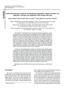
heteroskedasticity-robust standard errors. For completeness, in the Supplementary Material we also compare rejection probabilities and confidence intervals based on standard errors with finite-sample adjustments suggested by MacKinnon and White (1985), and we also replicate all experiments using MVR standard errors calculated under correct mean misspecification with the simplifications in (4.3). Figure 5.1 displays rejection probability curves of asymptotic t tests of the null hypothesis —4 = 1 for each sample size and value of the heteroskedasticity parameter –. The nominal size of the tests is set to 5%. Figures 5.1(a)-(d) show that MVR addresses overrejection of the OLS- and WLS-based tests in the presence of heteroskedasticity (– > 0). A striking feature of MVR rejection probability curves is that they flatten

25

very quickly across – as n increases, a feature somewhat more pronounced for ¸-MVR curves. This is in sharp contrast with OLS and e-WLS rejection probability curves that are increasing with the degree of heteroskedasticity –. For ¸-WLS the rejection curves are distorted around – = 1, for which it is efficient, and overall the rejection probabilities are much larger than for ¸-MVR. The curves for ¸-MVR and ¸-WLS coincide only for the case where ¸-MVR is efficient (– = 1) at moderate sample size and above (n Ø 320). The ¸-MVR rejection probability curve for n = 20 (black curve) is not placed above the other curves although it is above the nominal level for all values of –. This feature disappears when finite-sample corrections are implemented (Figures 2.1-2.3 in the Supplementary Material). In order to further investigate the relative performance of MVR-based inference, Tables 4 and 5 report the ratio of average MVR confidence interval lengths across simulations over the average OLS and WLS confidence interval lengths for —4 for each sample size and value of heteroskedasticity index –, in percentage terms. We find that in the presence of heteroskedasticity, the length of MVR confidence intervals is shorter for all designs compared to both OLS and WLS confidence intervals for some n large enough. The only exception is relative to ¸-WLS for – = 0.5, 1, as expected for – = 1 from ¸-WLS being efficient in that case. The relatively larger average length of the confidence intervals for ¸-MVR when n = 20 in Tables 4 and 5 is very much reduced with finite-sample corrections (Tables 1-4 in the Supplementary Material). Overall these simulation results demonstrate that MVR achieves large improvements in terms of estimation and inference compared to OLS in the presence of heteroskedasticity, and compared to WLS when the conditional variance function is misspecified. Our numerical simulations confirm MVR robustness to the specification of the scale function, and both ¸-MVR and e-MVR perform very well in finite samples. In the presence of heteroskedasticity rejection probabilities for MVR are much closer to nominal level than those for OLS and for WLS with misspecified weights. MVR achieves these improvements while simultaneously displaying tighter confidence intervals in all designs for sample sizes large enough. They are also shorter than their WLS counterpart with misspecified weights for sample sizes large enough. The precision of MVR estimates measured in RMSE is also largely superior to OLS under heteroskedasticity and to WLS with misspecified weights, with lower losses than WLS relative to OLS under homoskedasticity. These results and the simulations in the Supplementary Material illustrate the higher precision, improved finite-sample inference, and favorable approximation properties of MVR compared to classical least-squares methods.

26

0.4

0.4

0.3

0.3

0.2

0.2

0.1

0.1

0.0

0.0 0.0

0.5

1.0

1.5

2.0

0.0

0.5

α

0.4

0.3

0.3

0.2

0.2

0.1

0.1

0.0

0.0 1.0

2.0

(b) e-MVR vs OLS.

0.4

0.5

1.5

α

(a) ¸-MVR vs OLS.

0.0

1.0

1.5

2.0

0.0

α

0.5

1.0

1.5

α

(c) ¸-MVR vs ¸-WLS.

(d) e-MVR vs e-WLS.

Figure 5.1. Rejection frequencies for asymptotic t tests calculated with asymptotic standard errors: ¸-MVR and e-MVR (solid lines), and OLS and WLS (dashed lines). Sample sizes: 20 (black), 40 (red), 80 (green), 160 (blue), 320 (cyan), 640 (magenta), 1280 (grey).

27

2.0

¸-MVR –

0

n = 20 n = 40 n = 80 n = 160 n = 320 n = 640 n = 1280

204.1 121.0 106.7 102.9 101.4 100.6 100.4

0.5

1

e-MVR 1.5

2

193.8 179.9 167.2 158.7 117.5 109.8 100.0 91.0 105.9 97.7 85.5 75.0 101.8 90.1 74.8 64.0 98.5 83.1 65.6 55.3 95.2 76.2 57.5 47.8 92.1 70.1 50.5 41.3

0 114.7 104.2 101.6 100.9 100.6 100.2 100.2

0.5

1

1.5

2

121.8 123.2 123.4 121.9 109.8 108.8 103.1 94.1 106.0 100.7 89.1 74.3 103.3 92.9 76.4 59.1 100.0 84.8 65.1 47.3 96.3 77.0 55.6 38.2 93.0 70.3 47.9 31.1

Table 4. Ratio (◊100) of MVR average confidence interval lengths for —4 over corresponding OLS counterpart. Confidence intervals constructed with asymptotic standard errors. ¸-MVR –

0

0.5

1

n = 20 n = 40 n = 80 n = 160 n = 320 n = 640 n = 1280

245.2 140.4 120.5 112.7 108.7 105.5 103.4

226.0 128.8 111.5 105.7 103.4 102.7 102.7

210.7 123.4 109.8 106.3 105.4 105.1 104.9

e-MVR 1.5

2

201.3 197.4 120.1 117.0 107.5 103.2 101.9 96.7 98.3 92.7 95.3 89.0 93.0 85.4

0

0.5

1

136.1 113.0 105.7 102.8 101.4 100.7 100.4

143.3 118.8 110.7 106.8 103.9 101.2 98.9

149.8 126.1 116.1 108.6 102.0 95.8 90.5

1.5

2

158.7 165.9 132.7 133.8 119.4 113.5 107.2 96.1 96.5 81.8 87.0 70.1 79.4 60.9

Table 5. Ratio (◊100) of MVR average confidence interval lengths for —4 over corresponding WLS counterpart. Confidence intervals constructed with asymptotic standard errors.

6. Conclusion We introduce a new loss function for the linear estimation and approximation of CMFs. The proposed alternative generalises OLS, resulting in more robust approximations under misspecification and large improvements in finite samples. Given the importance of the least-squares loss in econometrics and statistics, and the common occurence of heteroskedasticity in empirical practice, the range of applications for simultaneous mean-variance regression will be vast. Examples of natural avenues for future research include the method of instrumental variables, GARCH models, and flexible specification of the conditional variance function for efficient estimation. These extensions will be considered in subsequent work.

28

Appendix A. Theory for the MVR Criterion A.1. Notation and Definitions. We define YA

1 ] Y ≠ X Õ— L(X, Y, ◊) := [ 2 s(X Õ “)

and

I

B2

Z ^

+ 1\ s(X Õ “), J

1 E[(Y ≠ X Õ —)2 | X] Â L(X, ◊) := + s(X Õ “) . Õ 2 s(X “) so that by iterated expectations the objective function can be expressed as Â Q(◊) = E[L(X, Y, ◊)] = E[L(X, ◊)],

◊œ

.

We denote the level sets of Q(◊) by Bc = {◊ œ : Q(◊) Æ c}, c œ R, with boundary set ˆBc . We also define the compact set B = B— ◊ B“ ™ , where B— and B“ are compact subsets of Rk and “ , respectively, and the boundary set of ˆ

= Rk ◊ ˆ

“,

ˆ

“

Ó

Ô

= “ œ Rk : Pr[s(X Õ “) = 0] > 0 .

For any two real numbers a and b, a ‚ b = max(a, b). For two random variables U and V , U denotes the support of U , defined as the set of values of U such that the density fU (u) of U is bounded away from 0, and Uv is the conditional support of U given V = v, v œ V. Throughout, C is a generic constant whose value may change from place to place.

A.2. Preliminary Results. This section gathers two preliminary results used in establishing the properties of Q(◊). Lemma 1. Let V be a random k vector such that E[V V Õ ] exists and is nonsingular. Then, for every sequence (“n ) in Rk such that ||“n || æ Œ, there exists v ú œ V such that lim||“n ||æŒ |“nÕ v ú | = Œ a.s. Proof. Consider a sequence (“n ) in Rk such that ||“n || æ Œ, and define ”n = ||““nn || . The sequence (”n ) is bounded, and by application of the Bolzano-Weierstrass theorem there exists a convergent subsequence ”nl , nl æ Œ as l æ Œ, with limit ”o . Moreover, E[V V Õ ] nonsingular implies that it is positive definite, so that E[(V Õ ”o )2 ] = ”oÕ E[V V Õ ]”o > 0. It follows that V Õ ”o ”= 0 on a set of positive probability, and

29

there exists a value v ú œ V such that ”oÕ v ú ”= 0 a.s. Therefore, ”nl = fies ”nÕ l v ú æ ”oÕ v ú ”= 0 as l æ Œ, which implies that limlæŒ |“nÕ l v ú | æ Œ: lim

læŒ

|“nÕ l v ú |

= lim

læŒ

The stated result follows.

- Õ ú -(”nl v )||“nl ||-

=

- Õ ú -(” v ) lim ||“n ||- o l læŒ

“nl ||“nl ||

satis-

= Œ. ⇤

Lemma 2. Suppose that Assumptions 1, 2 and 4 hold. Then the matrix S

Œ (◊) = E U

XX Õ s(X Õ “) Õ

XX Õ s (X s(X Õ “) 1

“)e(Y, X, ◊)

XX Õ s (X Õ “)e(Y, X, ◊) s(X Õ “) 1 € XX {s1 (X Õ “)e(Y, X, ◊)}2 s(“·X)

defined for all ◊ œ B, is positive definite.

T

V,

Proof. The proof builds on the proofs of Lemma S3 in Spady and Stouli (2018) and Theorem 1 in Newey and Stouli (2018). Positive definiteness of E[XX Õ /s(X Õ “)] for “ œ B“ under Assumption 4 implies that Œ (◊) is positive definite for all ◊ œ B if and only if the Schur complement of E[XX Õ /s(X Õ “)] in Œ (◊) is positive definite (Boyd and Vandenberghe, 2004, Appendix A.5.5) for all ◊ œ B, i.e., if and only if C

XX Õ Ã (◊) := E {s1 (X Õ “)e(Y, X, ◊)}2 s(X Õ “) C

D

D

C

XX Õ XX Õ Õ ≠E s (X “)e(Y, X, ◊) E 1 s(X Õ “) s(X Õ “)

D≠1

C

D

XX Õ E s1 (X Õ “)e(Y, X, ◊) s(X Õ “)

satisfies det{Ã (◊)} > 0, for all ◊ œ B. Letting

C

D

C

XX Õ XX Õ Õ (◊) := E s1 (X “)e(Y, X, ◊) E s(X Õ “) s(X Õ “) for all ◊ œ B, Ã (◊) is equal to SI

Xs1 (X Õ “)e(Y, X, ◊) X EU ≠ (◊) Õ 1/2 s(X “) s(X Õ “)1/2

JI

D≠1

,

Xs1 (X Õ “)e(Y, X, ◊) X ≠ (◊) Õ 1/2 s(X “) s(X Õ “)1/2

JÕ T

a finite positive definite matrix, if and only if for all ⁄ ”= 0 and all ◊ œ B there is no d such that (A.1)

Pr

CI

J

⁄Õ X s1 (X Õ “)e(Y, X, ◊) = dÕ s(X Õ “)1/2

I

X (◊) s(X Õ “)1/2

JD

> 0;

this is an application of the Cauchy-Schwarz inequality for matrices stated in Tripathi (1999).

30

V,

Positive definiteness of E [XX Õ /s(X Õ “)] for “ œ B“ under Assumption 4 implies that E [{⁄Õ X}2 /s(X Õ “)] > 0 for all ⁄ ”= 0, which implies that Pr[⁄Õ X/s(X Õ “)1/2 ”= 0] > 0 for all ⁄ ”= 0. Also, by Assumptions 1-2, we have Pr[s1 (X Õ “) > 0] = 1 and SA

s1 (X Õ “) Pr [Var(s1 (X Õ “)e(Y, X, ◊) | X) > 0] = Pr U s(X Õ “)

B2

T

Var(Y | X) > 0V = 1.

Thus for all ⁄ ”= 0, by (◊) being a constant matrix for all ◊ œ B, there is no d such that (A.1) holds, and the result follows. ⇤ A.3. Main Properties of Q(◊). Lemma 3. [Continuity] Suppose that Assumptions 1 and 3 hold. Then ◊ ‘æ Q(◊) is continuous over B. Proof. We first show that E[sup◊œB |L(X, Y, ◊)|] < Œ for all ◊ œ B. By the Triangle Inequality, (A.2)

2 |L(X, Y, ◊)| Æ |e(Y, X, ◊)2 s(X Õ “)| + |s(X Õ “)|.

Compactness of B“ implies that there exists a constant C such that sup“œB“ 1/s(X Õ “) Æ C < Œ a.s. Thus for ◊ œ B, the bound (A.3)

|e(Y, X, ◊)2 s(X Õ “)| Æ C[2Y 2 + 2(X Õ —)2 ] Æ 2C[Y 2 + sup ||—||2 ||X||2 ], —œB—

and sup—œB— ||—|| < Œ together imply that E[sup—œB |e(Y, X, ◊)2 s(X Õ “)|] < Œ requires E[Y 2 ] < Œ and E||X||2 < Œ, which hold under Assumption 3(i). It remains to show that E[sup“œB“ |s(X Õ “)|] < Œ. For “ œ B“ , some 0 Æ Ÿ œ (a, Œ) and some intermediate values “¯ , a mean-value expansion about (Ÿ, 0k≠1 )Õ yields |s(X Õ “)| = |s(Ÿ) + s1 (X Õ “¯ )(X Õ “ ≠ Ÿ)| Æ s(Ÿ) + sup ||“|| ||X||s1 (X Õ “¯ ). “œB“

With s(Ÿ), sup“œB“ ||“|| < Œ, E[sup“œB“ |s(X Õ “)|] < Œ requires E[||X||s1 (X Õ “¯ )] < Œ, which holds under Assumption 3(ii). Bound (A.2) now implies that E[sup◊œB |L(X, Y, ◊)|] < Œ, and continuity of Q(◊) then follows from continuity of ◊ ‘æ L(X, Y, ◊) and dominated convergence. ⇤ Lemma 4. [Continuous Di↵erentiability] If Assumptions 1 and 3 hold, then, for all ◊ œ B, Q(◊) is continuously di↵erentiable and Ê[L(X, Y, ◊)]/ˆ◊ = E[ˆL(X, Y, ◊)/ˆ◊].

31

Proof. We first show that E[sup◊œB ||ˆL(X, Y, ◊)/ˆ◊||] < Œ. Computing

1 ˆL(X, Y, ◊)/ˆ“ = ≠ Xs1 (X Õ “){e(Y, X, ◊)2 ≠ 1}. 2 Compactness of B“ implies that there exists a constant C such that sup“œB“ 1/s(X Õ “) Æ C < Œ a.s. Thus for ◊ œ B, the bound ˆL(X, Y, ◊)/ˆ— = ≠Xe(Y, X, ◊),

||Xe(Y, X, ◊)|| Æ C||X|| |Y ≠ X Õ —| Æ C[|Y | ||X|| + sup ||—|| ||X||2 ], —œB—

and sup—œB— ||—|| < Œ, imply that E[sup◊œB ||ˆL(X, Y, ◊)/ˆ—||] < Œ requires E[|Y | ||X||] < Œ and E||X||2 < Œ, which hold under Assumptions 3(i). We now show that E[sup◊œB ||ˆL(X, Y, ◊)/ˆ“||] < Œ. Since ≠1 Æ e(Y, X, ◊)2 ≠ 1 a.s., for ◊ œ B, . . .Xs1 (X Õ “){e(Y, X, ◊)2

(A.4)

. .

≠ 1}. Æ ||X|| s1 (X Õ “) |e(Y, X, ◊)2 ≠ 1|

Æ ||X|| s1 (X Õ “) [1 ‚ 2C(Y 2 + sup ||—||2 ||X||2 )]. —œB—

For “ œ B“ , some 0 Æ Ÿ œ (a, Œ) and some intermediate values “¯ , a mean-value expansion about (Ÿ, 0k≠1 )Õ yields (A.5)

|s1 (X Õ “)| = |s1 (Ÿ) + s2 (X Õ “¯ )(X Õ “ ≠ Ÿ)| Æ s1 (Ÿ) + sup ||“|| ||X||s2 (X Õ “¯ ). “œB“

This bound and (A.4) together imply

(A.6)

. . .Xs1 (X Õ “){e(Y, X, ◊)2

. .

≠ 1}. Æ ||X|| [s1 (Ÿ) + sup ||“|| ||X||s2 (X Õ “¯ )] “œB“

2

◊[1 ‚ 2C(Y + sup ||—||2 ||X||2 )]. —œB—

Since B is compact and 0 < s1 (Ÿ) < Œ, E[sup◊œB ||Ò“ L(X, Y, ◊)||] < Œ requires E||X||3 < Œ, E[Y 2 ||X||] < Œ and, for all “ œ B“ , E[ÎXÎ4 s2 (X Õ “)] < Œ and E[Y 2 ||X||2 s2 (X Õ “)] < Œ, which hold under Assumption 3. We have shown that E[sup◊œB ||ˆL(X, Y, ◊)/ˆ◊||] < Œ and it now follows by Lemma 3.6 in Newey and Mc Fadden (1994) that Q(◊) is continuously di↵erentiable over B, and that the order of di↵erentiation and integration can be interchanged. ⇤ Lemma 5. [Convexity] Suppose that Assumptions 1, 3 and 4 hold. Then ◊ ‘æ Q(◊) is strictly convex over B.

32

Proof. Q(◊) is di↵erentiable for all ◊ œ B and the order of integration and di↵erentiation can be interchanged by Lemma 4. In order to show that ˆQ(◊)/ˆ◊ is differentiable for ◊ œ B, we show that E[sup◊œB ||ˆ 2 L(X, Y, ◊)/ˆ◊ˆ◊||] < Œ. Direct calculations yield 2

ˆ L(X, Y, ◊) ˆ◊ˆ◊

S

= U

XX Õ s(X Õ “) Õ

XX Õ s (X s(X Õ “) 1

“)e(Y, X, ◊)

S

XX Õ s (X Õ “)e(Y, X, ◊) s(X Õ “) 1 XX Õ {s1 (X Õ “)e(Y, X, ◊)}2 s(X Õ “)

T

0k◊k 0k◊k V +U 1 Õ Õ 0k◊k ≠ 2 XX s2 (X “){e(Y, X, ◊)2 ≠ 1}

T V

=: h1 (X, Y, ◊) + h2 (X, Y, ◊).

We first consider E[sup◊œB ||ˆ 2 h1 (X, Y, ◊)/ˆ◊ˆ◊||]. Steps similar to those leading to (A.3) imply that E[sup◊œB ||ˆ 2 h1 (X, Y, ◊)/ˆ—ˆ—||] < 2 Œ is satisfied since E||X|| < Œ and B is compact. Moreover, 2 2 E[sup◊œB ||ˆ h1 (X, Y, ◊)/ˆ—ˆ“||] < Œ and E[sup◊œB ||ˆ h1 (X, Y, ◊)/ˆ“ˆ—||] < Œ are implied by E[sup◊œB ||ˆ 2 h1 (X, Y, ◊)/ˆ“ˆ“||] < Œ. Steps similar to those leading to (A.6) yield, for ◊ œ B, . . . XX Õ . . Õ 2. . {s (X “)e(Y, X, ◊)} . 1 . s(X Õ “) .

Æ C||X||2 s1 (X Õ “)2 [Y 2 + sup ||—||2 ||X||2 ]. —œB—

This bound and expansion (A.5) together imply, for some 0 Æ Ÿ œ (a, Œ) and some intermediate value “¯ , . . . XX Õ . . Õ 2. . {s (X “)e(Y, X, ◊)} . . s(X Õ “) 1 .

Æ C||X||2 [s1 (Ÿ)2 + 2 sup ||“|| ||X||s1 (X Õ “¯ )s2 (X Õ “¯ )] “œB“

◊ [Y 2 + sup ||—||2 ||X||2 ]. —œB—

Since B is compact and 0 < s1 (Ÿ) < Œ, E[sup◊œB ||ˆ 2 h1 (X, Y, ◊)/ˆ“ˆ“||] < Œ requires E||X||4 < Œ, E[Y 2 ||X||2 ] < Œ and, for all “ œ B“ , E[ÎXÎ5 s1 (X Õ “)s2 (X Õ “)] < Œ and E [Y 2 ||X||3 s1 (X Õ “)s2 (X Õ “)] < Œ, which hold under Assumption 3. We now show that E[sup◊œB ||ˆ 2 h2 (X, Y, ◊)/ˆ◊ˆ◊||] < Œ. It suffices to show that E[sup◊œB ||ˆ 2 h2 (X, Y, ◊)/ˆ“ˆ“||] < Œ. Steps similar to those leading to (A.6), yield, for ◊ œ B, (A.7)

. . .XX Õ s2 (X Õ “){e(Y, X, ◊)2

.

≠ 1}.. Æ ||X||2 s2 (X Õ “)[1 ‚ 2C(Y 2 + sup ||—||2 ||X||2 )]]. —œB—

33

For “ œ B“ a mean-value expansion about (Ÿ, 0k≠1 )Õ yields

|s2 (X Õ “)| = |s2 (Ÿ) + s3 (X Õ “¯ )(X Õ “ ≠ Ÿ)| Æ s2 (Ÿ) + sup ||“|| ||X||s3 (X Õ “¯ ) “œB“

This bound and (A.7) together imply . . .XX Õ s2 (X Õ “){e(Y, X, ◊)2

.

≠ 1}.. Æ ||X||2 [s2 (Ÿ) + sup ||“|| ||X||s3 (X Õ “¯ )] “œB“

2

◊[1 ‚ 2C(Y + sup ||—||2 ||X||2 )]. —œB—

Since B is compact and 0 Æ s2 (Ÿ) < Œ, E[sup◊œB ||ˆ 2 h2 (X, Y, ◊)/ˆ“ˆ“||] < Œ requires E||X||4 < Œ, E[Y 2 ||X||2 ] < Œ and, for all “ œ B“ , E[ÎXÎ5 s3 (X Õ “)] < Œ and E[Y 2 ||X||3 s3 (X Õ “)] < Œ, which hold under Assumption 3.

We have shown that E[sup◊œB ||ˆ 2 L(X, Y, ◊)/ˆ◊ˆ◊||] < Œ and it follows by Lemma 3.6 in Newey and Mc Fadden (1994) that ˆQ(◊)/ˆ◊ is continuously di↵erentiable over B, and that the order of di↵erentiation and integration can be interchanged.

Letting H1 (◊) := E[h1 (X, Y, ◊)] and H2 (◊) := E[h2 (X, Y, ◊)], for all ◊ œ B, the Hessian matrix of Q(◊) is H(◊) := H1 (◊) + H2 (◊), which is positive semidefinite if H1 (◊) and H2 (◊) are positive semidefinite (Horn and Johnson, 2012, p.398, 7.1.3. observation). And if either one of H1 (◊) and H2 (◊) is positive definite (while the other is positive semidefinite), then H(◊) is positive definite. All principal minors of H2 (◊) have determinant 0 for all ◊ œ B, and H2 (◊) is thus positive semidefinite. Applying Lemma 2 with Œ (◊) = H1 (◊), we have that H1 (◊) is positive definite for all ◊ œ B. We conclude that H(◊) is positive definite for all ◊ œ B, and the result follows. ⇤ Lemma 6. [Level Sets Compactness] If Assumptions 1, 3 and 4 hold then the level sets of ◊ ‘æ Q(◊) are compact. Proof. We show that the level sets Bc , c œ R, of ◊ ‘æ Q(◊) are closed and bounded. The result then follows by the Heine-Borel theorem. Step 1. [Bc is bounded]. We show that every sequence in Bc is bounded. Suppose the contrary. Then there exists an unbounded sequence (◊n ) in Bc , and a subsequence (◊nl ), nl æ Œ as l æ Œ, such that either ||—nl || æ Œ or ||“nl || æ Œ.

Step 1.1. If ||“nl || æ Œ, then E[XX Õ ] nonsingular implies that there exists a value xú œ X such that |“nÕ l xú | æ Œ as l æ Œ, a.s., by Lemma 1, which implies s(“nÕ l xú ) æ 0 or Œ by definition of t ‘æ s(t) in Assumption 1.

34

Moreover, for xú œ X such that |“nÕ l xú | æ Œ as l æ Œ, we have that E[(Y ≠ X Õ —)2 | X = xú ] < Œ for all — œ Rk under Assumption 3(i). It follows that for all — œ Rk , (A.8)

Õ 2 ú ˜ ú , —, “n ) = 1 lim E[(Y ≠ X —) | X = x ] + 1 lim s(“ Õ xú ) = Œ. lim L(x nl l læŒ 2 læŒ s(“nÕ l xú ) 2 læŒ

˜ Since L(X, ◊) is positive a.s. for all ◊ œ and the density fX (x) is bounded away from ˜ 0 for all x œ X by definition of X , (A.8) implies that E[limlæŒ L(X, —, “nl )] = Œ. ˜ Since E[L(X, ◊)] = Q(◊), Fatou’s lemma then implies that limlæŒ Q(—, “nl ) = Œ, for k all — œ R . Therefore “ is bounded. Step 1.2. If ||—nl || æ Œ, then E[XX Õ ] nonsingular implies that there exists a value xúú œ X such that |—nÕ l xúú | æ Œ a.s., by a second application of Lemma 1. Thus (Y ≠ —nÕ l xúú )2 æ Œ as l æ Œ a.s. Moreover, for xúú œ X such that |—nÕ l xúú | æ Œ as l æ Œ, we have that E[limlæŒ (Y ≠ X Õ —nl )2 | X = xúú ] = Œ, and Fatou’s lemma then implies that limlæŒ E[(Y ≠X Õ —nl )2 | X = xúú ] = Œ. Also, s(“ Õ xúú ) is finite and positive for any “ œ “ . It follows that for all “ œ “ , (A.9)

Õ 2 úú ˜ úú , —n , “) Ø 1 lim E[(Y ≠ X —nl ) | X = x ] = Œ. lim L(x l læŒ 2 læŒ s(“ Õ xúú )

˜ Since L(X, ◊) is positive a.s. for all ◊ œ and the density fX (x) is bounded away from ˜ 0 for all x œ X by definition of X , (A.9) implies that E[limlæŒ L(X, —nl , “)] = Œ. ˜ Fatou’s lemma then implies that limlæŒ E[L(X, —nl , “)] = limlæŒ Q(—nl , “) = Œ for all “ œ “ . Therefore — is bounded. Step 2. [Bc is closed]. We examine the behaviour of ◊ ‘æ Q(◊) on the boundary set ˆ in order to determine whether Bc is closed. We show that for every sequence in Bc converging to a boundary point in ˆ , ◊ ‘æ Q(◊) is unbounded. Continuity of ◊ ‘æ Q(◊) established in Lemma 3 then implies that Bc is closed. Consider a sequence ◊n in Bc such that ◊n æ to œ ˆ as n æ Œ. Then, there exists xú œ X such that “nÕ xú æ 0 as n æ Œ a.s., by definition of ˆ . Moreover, E[(Y ≠ X Õ —)2 |X] > 0 a.s. for all — œ Rk under Assumption 2. Thus (A.10)

˜ ú , ◊n ) = lim L(x næŒ

1 E[(Y ≠ X Õ —n )2 | X = xú ] lim = Œ. 2 næŒ “nÕ xú

˜ Since L(X, ◊) is positive a.s. for all ◊ œ and the density fX (x) is bounded away ˜ from 0 for all x œ X by definition of X , (A.10) implies that E[limnæŒ L(X, ◊n )] = Œ. ˜ Fatou’s lemma then implies that limnæŒ E[L(X, ◊n )] = limnæŒ Q(◊n ) = Œ. This

35

yields a contradiction since Q(◊n ) Æ c for ◊n œ Bc . Moreover, continuity of ◊ ‘æ Q(◊) implies Q(to ) = limnæŒ Q(◊n ) Æ c. Therefore, to œ Bc and Bc is closed. ⇤ Appendix B. Proofs for Sections 2 and 3 B.1. Proof of Theorem 1. Under Assumptions 1-4, the order of integration and di↵erentiation for the MVR population problem (2.2) can be interchanged by Lemma 4. Therefore the first-order conditions of problem (2.2) are (2.3)-(2.4), which are satisfied by ◊0 . Uniqueness follows from strict convexity of Q(◊) over compact subsets of established in Lemma 5, and compactness of the level sets of the objective function Q(◊) established in Lemma 6. ⇤ B.2. Proof of Proposition 1. The first-order conditions (2.3)-(2.4) of the MVR population problem (2.2) can be written as (B.1) (B.2)

C

C

D

X E (Y ≠ X Õ —) Õ s(X “)

D

Ô s1 (X Õ “) Ó Õ 2 Õ 2 E X (Y ≠ X —) ≠ s(X “) s(X Õ “)2

= 0 = 0,

with unique solutions —0 and “0 , by Theorem 1. Under the stated assumptions, the first-order conditions of problem (2.8)-(2.9) are (B.3) (B.4)

C

C

D

X E (Y ≠ X Õ —) ‡(X)

D

Ô s(X Õ “)s1 (X Õ “) Ó Õ 2 Õ 2 ≠4E X (Y ≠ X — ) ≠ s(X “) 0 ‡(X)3

= 0 = 0.

By assumption the variance of Y conditional on X is correctly specified and ‡(X)2 = s(X Õ “0 )2 a.s. Conditions (B.3)-(B.4) are therefore satisfied for (—, “) = (—0 , “0 ), and are then equivalent to the MVR first-order conditions (B.1)-(B.2) evaluated at the solution (—, “) = (—0 , “0 ). ⇤ B.3. Proof of Theorem 2. Step 1: Existence. Pick c œ R such that the level set Bc = {◊ œ : Q(◊) Æ c} is nonempty. By Lemma 6, Bc is compact. Continuity of ◊ ‘æ Q(◊) over compact subsets of established in Lemma 3 then implies that there exists at least one minimizer to Q(◊) in Bc by the Weierstrass extreme value theorem. Minimizing Q(◊) over is equivalent to minimizing Q(◊) over any of its nonempty level sets, which establishes existence of a minimizer ◊ú œ .

36

Step 2: Uniqueness. By Lemma 5, we have that ◊ ‘æ Q(◊) is strictly convex over compact subsets of , and thus over Bc , so that Q(◊) admits at most one minimizer in Bc . This establishes uniqueness of a minimizer ◊ú œ . ⇤ B.4. Proof of Theorem 3. Proof of part (i). For ◊ œ , define the function Z A B2 ˆ Y Õ 2 ] ^ 1 µ(x) ≠ x — ‡(x) Â Q(◊) := + + 1 s(xÕ “)dFX (x). Õ Õ 2 [ \ 2 s(x “) s(x “) Â We show that Q(◊) is equal to Q(◊) for all ◊ œ

.

The location-scale representation (3.1) for Y | X implies that, for ◊ œ A

Y ≠ X Õ— s(X Õ “)

B2

(B.5)

=

A

=

A

[µ(X) ≠ X Õ —] + ‡(X)Á s(X Õ “) µ(X) ≠ X Õ — s(X Õ “)

B2

,

B2

A

µ(X) ≠ X Õ — +2 s(X Õ “)

B

‡(X) ‡(X)2 2 Á + Á, s(X Õ “) s(X Õ “)2

and the change of variable formula fY |X (Y | X) = fÁ|X

(B.6)

A

Y ≠ µ(X) |X ‡(X)

BA

B

1 , ‡(X)

hold a.s. The definition of ˆ 1 Q(◊) = 2 ˆ 1 = 2 ˆ 1 = 2

Q(◊) and expressions (B.5)-(B.6) together imply, for ◊ œ YA ] y

≠ xÕ — s(xÕ “)

B2

≠ xÕ — s(xÕ “)

B2

[ YA ] y

Z ^

+ 1 s(xÕ “)fY |X (y | x)dydFX (x) \ Z ^

+ 1 s(x “)f Õ

A

y ≠ µ(x) |x ‡(x)

Á|X [ \ YA B A B ] µ(x) ≠ xÕ — 2 µ(x) ≠ xÕ —

[

s(xÕ “)

,

+2

s(xÕ “)

BA

B

1 dydFX (x) ‡(x) Z

^ ‡(x) ‡(x)2 2 e + e + 1 \ s(xÕ “) s(xÕ “)2

◊s(xÕ “)fÁ|X (e | x) dedFX (x) Z B2 ˆ YA ^ 1 ] µ(x) ≠ xÕ — ‡(x)2 Â = + + 1 s(xÕ “)dFX (x) = Q(◊), \ 2 [ s(xÕ “) s(xÕ “)2

where the final step uses the law of iterated expectations and the mean zero and unit variance property of Á conditional on X. Since ◊ú is the unique minimizer of Q(◊) in Â , it is also the unique minimizer of Q(◊) in . ⇤ 37

Proof of part (ii). Since LS µ , and ◊ú and ◊LS are the unique minimizers of Q(◊) over and LS , respectively, it follows that Q(◊ú ) Æ Q(◊LS ). ⇤ B.5. Proof of Corollary 1. For the linear scale specification s(t) = t, conditions (2.4) imply E[(X Õ “ ú )e(Y, X, ◊ú )2 ] = E[X Õ “ ú ]. For the exponential scale specification s(t) = exp(t), because X includes an intercept, conditions (2.4) imply that E[exp(X Õ “ ú )e(Y, X, ◊ú )2 ] = E[exp(X Õ “ ú )]. It follows that for the linear and exponential scale specifications, E[s(X Õ “ ú )e(Y, X, ◊ú )2 ] = E[s(X Õ “ ú )], and 1 Q(◊ú ) = E[{e(Y, X, ◊ú )2 + 1}s(X Õ “ ú )] = E[s(X Õ “ ú )]. 2 We have shown that for the linear and exponential scale specifications, Q(◊ú ) = E[e(Y, X, ◊ú )2 s(X Õ “ ú )]. For OLS, conditions (2.4) simplify to E[e(Y, X, ◊LS )2 ≠ 1] = 0, which implies that s(“LS ) = E[(Y ≠ X Õ —LS )2 ]1/2 , and 1 Q(◊LS ) = E[{e(Y, X, ◊LS )2 + 1}s(“LS )] = s(“LS ). 2

We have shown that for the constant scale specification Q(◊LS ) = E[(Y ≠ X Õ —LS )2 ]1/2 . The result then follows by Theorem 3(ii). ⇤

B.6. Proof of Theorem 4. By Theorem 3(ii) we have that E [s(X Õ “ ú )] = Q(◊ú ) Æ Q(◊LS ) = ‡LS . This and Jensen’s inequality for concave functions imply that (B.7)

E [log s(X Õ “ ú )] Æ log E [s(X Õ “ ú )] Æ log (‡LS ) ,

by monotonicity of the logarithmic function. Thus ‘ = 2 {log (‡LS ) ≠ E [log s(X Õ “ ú )]} Ø 0.

By definition (3.6) of the Gaussian density, inequality (B.7), and E[e (Y, X, ◊LS )2 ] = 1, the bound E [e(Y, X, ◊ú )2 ] Æ 1 + ‘, implies 5

(B.8)

1 1 ≠E [log f◊ú (Y, X)] = log (2fi) + E log s(X Õ “ ú ) + e(Y, X, ◊ú )2 2 2 1 Æ [log (2fi) + 1] + log (‡LS ) 2 = ≠E [log f◊LS (Y, X)] .

6

Therefore, upon adding E[log fY |X (Y | X)] to each side of the inequality, we obtain inequality (3.8). ⇤

38

B.7. Proof of Corollary 2. By assumption µ(X) = X Õ —0 a.s., and by definition ◊ú satisfies conditions (3.3)-(3.4). Then the first-order conditions (3.3) are satisfied by — ú = —0 , and “ ú must satisfy C

I

JD

‡(X)2 E Xs1 (X “ ) ≠1 s(X Õ “ ú )2

(B.9)

Õ ú

= 0.

If there exists a pair (—, “) œ satisfying all 2 ◊ k conditions (3.3)-(3.4) simultaneously, then this pair is unique, by strict convexity of ◊ ‘æ Q(◊). It follows from the existence proof of Theorem 2 that the restriction q(“) := Q(◊)|—=—0 has a minimizer in ú “ , i.e., there exists “ such that (B.9) holds. Since “ ‘æ q(“) is also strictly convex, q(“) admits a unique minimizer “ ú (—0 ) in “ . Therefore, the pair (—0 , “ ú (—0 )) is the unique minimizer of Q(◊) when µ(X) = X Õ —0 a.s. ⇤ ´ B.8. Proof of Theorem 5. Letting L1 (X ) = {Â : |Â(x)| fX (x)dx < Œ}, define the set of admissible conditional standard deviation functions as Ó

Ô

S = Â œ L1 (X ) : Pr[Â(X) > 0] = 1 . We first show that ‡(X) is a minimizer of the MVR criterion S

YA

1 ] Y ≠ X Õ —0 Q0 (Â) := E U [ 2 Â(X)

B2

Z ^

T

+ 1\ Â(X)V ,

Â œ S.

Assuming that the order of di↵erentiation and integration can be interchanged, as in Lemma 4, and setting Â– (X) := ‡(X) + –Â(X) and e– (Y, X) := (Y ≠ X Õ —0 )/Â– (X), we have -

C

ˆQ0 (Â– ) -1 ê– (Y, X) ˆÂ– (X) ˆÂ– (X) = E 2e– (Y, X) Â– (X) + e– (Y, X)2 + ˆ– 2 ˆ– ˆ– ˆ– –=0 =

C

1 ˆÂ– (X) E ≠ 2 ˆ–

DÔ 2 e– (Y, X) ≠ 1 --

Ó

,

D-

–=0

–=0

upon using that ê– (Y, X)/ˆ– = ≠e– (Y, X){ˆÂ– (X)/ˆ–}{Â– (X)}≠1 . Therefore -

È ˆQ0 (Â– ) -1 Ë = E ≠Â(X){e(Y, X)2 ≠ 1} = 0, ˆ– -–=0 2

Y ≠ X Õ —0 e(Y, X) := , ‡(X)

for each Â œ S since E [e(Y, X)2 | X] = 1 implies that E [h(X) {e(Y, X)2 ≠ 1}] = 0 for any measurable function of X, and in particular each Â œ S. We next show that Q0 (Â) is strictly convex and thus admits at most one minimizer. Assuming that the order of di↵erentiation and integration can be interchanged, as in

39

Lemma 5, we have -

C

ˆ 2 Q0 (Â– ) -1 ê– (Y, X) = E ≠2Â(X)e– (Y, X) 2 ˆ– 2 ˆ– –=0 =

C

DÂ(X) 2 E e– (Y, X) -Â– (X) –=0 C D

=E

C

2

D-

–=0

Â(X)2 e(Y, X)2 ‡(X) D

Â(X)2 =E > 0, ‡(X) for each Â œ S. Therefore ‡(X) is the unique minimizer of Q0 (Â) in S.

Under correct specification of the CMF, we have that — ú = —0 , by Corollary 2. By s(X Õ “ ú ) œ S and ‡(X) being the unique minimizer of Q0 (Â) in S we have that Q0 (‡) Æ Q(◊ú ). By Q0 (‡) = E [‡(X)] and Q(◊ú ) = E [s(X Õ “ ú )], we have shown that E [‡(X)] Æ E [s(X Õ “ ú )]. This and Jensen’s inequality for concave functions imply (B.10)

E [log ‡(X)] Æ log E [‡(X)] Æ log E [s(X Õ “ ú )] ,

by monotonicity of the logarithmic function.

By iterated expectations and using that z ‘æ z ≠ 1 ≠ log z is a positive-valued strictly convex function for z Ø 0 gives the bound (B.11) SA B2 T Ë È ‡(X) ú 2 V Ø 1 + 2 {E [log ‡(X)] ≠ E [log s(X Õ “ ú )]} . E e(Y, X, ◊ ) = E U Õ ú s(X “ )

By definition of the Gaussian density, inequality (B.10), and E[e (Y, X)2 ] = 1, bound (B.11) implies 5

1 1 log (2fi) + E log s(X Õ “ ú ) + e(Y, X, ◊ú )2 2 2 1 Ø [log (2fi) + 1] + E [log ‡(X)] 2 Ë È = ≠E log f—†0 (Y, X) .

≠E [log f◊ú (Y, X)] =

(B.12)

Upon combining (B.8) and (B.12) we obtain inequality (3.11).

40

6

⇤

Appendix C. Asymptotic Theory Lemma 7. Suppose that Assumptions 1, 3 and 5 holds. Then Qn (◊) is strictly convex over B. Proof. For ei = e(yi , xi , ◊), the Hessian matrix Hn (◊) of Qn (◊), S

n 1ÿ U Hn (◊) = n i=1

xi xÕi s(xÕi “)

xi xÕi s (xÕ “)ei s(xÕi “) 1 i

S

xi xÕi s (xÕ “)ei s(xÕi “) 1 i xi xÕi {s1 (xÕi “)ei }2 s(xÕi “)

T

T V

n 0 0k◊k 1ÿ U k◊k V := H1n (◊) + H2n (◊), + 1 n i=1 0k◊k ≠ 2 xi xÕi s2 (xÕi “)(e2i ≠ 1)

defined for ◊ œ B, is positive definite. Steps similar to the proof of Lemma 2 show that H1n (◊) is positive definite for all ◊ œ B. Moreover, all principal minors of H2n (◊) have determinant 0 for all ◊ œ B, and H2n (◊) is thus positive semidefinite. Since Hn (◊) = H1n (◊) + H2n (◊), we conclude that Hn is positive definite for all ◊ œ B (Horn and Johnson, 2012, p.398, 7.1.3. observation), and the result follows. ⇤ C.1. Proof of Theorem 6. Proof of part (i)-(ii). By Theorem 2, ◊ú œ is the unique minimizer of Q(◊), and the identification condition (i) in Theorem 2.7 in Newey and Mc Fadden (1994) is thus verified. Since is convex and open, existence of ◊ú œ established in Theorem 2, as well as strict convexity of Qn (◊) established in Lemma 7 imply that their condition (ii) is satisfied. Finally, since the sample is i.i.d. by Assumption 5, pointwise convergence of Qn (◊) to Q0 (◊) follows from Q0 (◊) bounded (established in the proof of Lemma 3) and application of Khinchine’s law of large numbers. Hence, all conditions of Newey and McFadden’s Theorem 2.7 are satisfied. Therefore, there exists ◊ˆ œ with probability approaching one, and p ú ˆ ◊æ ◊ . ⇤ Proof of part (iii). The sample MVR solution ◊ˆ can be equivalently formulated as the Method-of-Moments estimator C

DÕ C

n 1ÿ ◊ˆ = arg min m(yi , xi , ◊) ◊œ« n i=1

D

n 1ÿ m(yi , xi , ◊) , n i=1

d The asymptotic normality result n1/2 (◊ˆ ≠ ◊ú ) æ N (0, G≠1 S(G≠1 )Õ ) then follows from this characterization upon verifying the assumptions of Theorem 3.4 in Newey and Mc Fadden (1994), for instance. Block symmetry of G then implies that V = G≠1 SG≠1 .

41

By Theorem 2, ◊ú is in the interior of so that their Condition (i) is satisfied. The mapping ◊ ‘æ m(Y, X, ◊) is continuously di↵erentiable, by inspection, so that their Condition (ii) is satisfied. By definition, ◊ú satisfies E[m(Y, X, ◊ú )] = 0, hence the first part of their condition (iii) is satisfied. Moreover, bound (A.6) in the proof of Lemma 4 and the steps below show that E[||m(Y, X, ◊ú )||2 ] is finite under Assumption 6, verifying their Condition (iii). Finally, under our assumptions, from the proof of Lemma 5, E[sup◊œ ||ˆm(Y, X, ◊)/ˆ◊||] = E[sup◊œ ||ˆ 2 L(X, Y, ◊)/ˆ◊ˆ◊||] is finite and G = E[ˆm(Y, X, ◊ú )/ˆ◊] is nonsingular. Their Conditions (iv) and (v) are satisfied. If µ(X) = X Õ — ú a.s., then E[(Y ≠ X Õ — ú )/s(X Õ “ ú ) | X] = 0. Therefore, by iterated expectations, the o↵-diagonal blocks of G and S simplify to (4.3). If µ(X) = X Õ — ú a.s. and ‡ 2 (X) = s(X Õ “ ú )2 a.s., then E[e2 ≠ 1 | X] = 0. Therefore, repeated use of iterated expectations imply C

D

5

6

C

D

XX Õ 1 XX Õ Õ ú 2 Õ Õ ú 2 E {s (X “ )e} ≠ E XX s (X “ )(e ≠ 1) = E s1 (X Õ “ ú )2 , 1 2 s(X Õ “ ú ) 2 s(X Õ “ ú ) which yields G22 in (4.4), and S11 and S22 in (4.4). Application of Theorem 4.5 in Newey and Mc Fadden (1994) implies that ˆ ≠1 SˆG ˆ ≠1 æp G≠1 SG≠1 . Under Assumption 6, steps similar to the proof of Lemma 4 G show that for a neighborhood N of ◊ú we have E[sup◊œN ||m(Y, X, ◊)||2 ] < Œ: bound (A.6) implies, for all ◊ œ N , . . .Xs1 (X Õ “){e(Y, X, ◊)2

.2 .

Ó

≠ 1}. Æ C[||X|| + ||X||s2 (X Õ “¯ )][Y 2 + ||X||2 ]

Ô2

Æ 2C[||X||2 + ||X||2 s2 (X Õ “¯ )2 ][Y 4 + ||X||4 ],

and E[sup◊œN ||m(Y, X, ◊)||2 ] < Œ requires E[Y 4 ||X||2 ] < Œ, E[||X||6 ] < Œ, and, for all “ œ “ , E[Y 4 ||X||2 s2 (X Õ “)2 ] < Œ, and E[||X||6 s2 (X Õ “)2 ] < Œ. By Holder’s inequality E[Y 4 ||X||2 ] < Œ and E[Y 4 ||X||2 s2 (X Õ “)2 ] < Œ if E[Y 6 ] < Œ, E[||X||6 ] < Œ, and E[||X||6 s2 (X Õ “)6 ] < Œ, which hold under Assumption 6. Moreover, ◊ ‘æ m(Y, X, ◊) is continuous at ◊ú a.s. The result follows. ⇤

References Acemoglu, D., Johnson, S. and Robinson, J. (2002). Reversal of Fortune: Geography and Institutions in the Making of the Modern World Income Distribution. Quarterly Journal of Economics 117, pp. 1231–1294.

42

Akaike, H. (1973). Information Theory and an Extension of the Likelihood Principle. In Proceedings of the Second International Symposium of Information Theory, ed. by B. N. Petrov, and F. Csaki. Angrist, J. and Krueger, A. (1999). Empirical Strategies in Labor Economics. In Handbook of Labor Economics, Vol. 3, pp. 1277–1366. Amsterdam: Elsevier. Angrist, J. D. and Pischke, J. S. (2008). Mostly Harmless Econometrics: An Empiricist’s Companion. Princeton University. Blundell, R., Horowitz, J. and Parey, M. (2012). Measuring the Price Responsiveness of Gasoline Demand: Economic Shape Restrictions and Nonparametric Demand Estimation. Quantitative Economics 3, pp. 29–51. Boyd, S. P. and Vandenberghe, L. (2004). Convex Optimization. Cambridge University Press. Breusch, T. S. and Pagan, A. R. (1979). A Simple Test for Heteroscedasticity and Random Coefficient Variation. Econometrica (47, September), pp. 1287–1294. Cameron, A. C. and Trivedi, P. K. (2005). Microeconometrics: Methods and Applications. Cambridge University Press. Chamberlain, G. (1984). Panel Data. In Handbook of Econometrics, Vol. 2, ed. by Z. Griliches and M. Intriligator. Amsterdam: North-Holland, pp. 1247–1318. Chesher, A. (1989). Hajek Inequalities, Measures of Leverage and the Size of Heteroskedasticity Robust Tests. Journal of Econometrics 57, pp. 971–977. Chesher, A. and Austin, G. (1991). The Finite-Sample Distributions of Heteroskedasticity Robust Wald Statistics. Journal of Econometrics 47, pp. 153–173. Chesher, A. and Jewitt, I. (1987). The Bias of a Heteroskedasticity Consistent Covariance Matrix Estimator. Econometrica (55, September), pp. 1217–1222. Chesher, A. and Spady, R. H. (1991). Asymptotic Expansions of the Information Matrix Test Statistic. Econometrica (59, May), pp. 787–815. Eicker, H. (1963). Asymptotic Normality and Consistency of the Least-Squares Estimators for Families of Linear Regressions. The Annals of Mathematical Statistics 34, pp. 447–456. Eicker, H. (1967). Limit Theorems for Regressions with Unequal and Dependent Errors. In Proceedings of the fifth Berkeley symposium on mathematical statistics and probability, Vol. 1, pp. 59–82. Horn, R. A. and Johnson, C. R. (2012). Matrix Analysis. 2nd ed., Cambridge University Press. Huber, P. (1967). The Behavior of Maximum Likelihood Estimates under Nonstandard Conditions. In Proceedings of the fifth Berkeley symposium on mathematical

43

statistics and probability, Vol. 1, pp. 221–233. Huber, P. (1981). Robust Statistics. Wiley, New York. Koenker, R. (1981). A Note on Studentizing a Test for Heteroscedasticity. Journal of Econometrics 17, pp. 107–112. Koenker, R. (2005). Quantile Regression. Econometric Society Monograph Series, Vol. 38. Cambridge University Press. MacKinnon, J. G. (2013). Thirty Years of Heteroskedasticity-Robust Inference. In Recent advances and future directions in causality, prediction, and specification analysis, pp. 437-461. Springer, New York, NY. MacKinnon, J. G. and White, H. (1985). Some Heteroskedasticity-Consistent Covariance Matrix Estimators with Improved Finite Sample Properties. Journal of Econometrics 29, pp. 305–325. Newey, W. and Mc Fadden, D. (1994). Large Sample Estimation and Hypothesis Testing. In Handbook of Econometrics, Vol. 4, ch. 36, 1st ed., pp. 2111–2245. Amsterdam: Elsevier. Newey, W. and Stouli, S. (2018). Control variables, discrete instruments, and identification of structural functions. arXiv preprint arXiv:1809.05706. Owen, A. B. (2007). A Robust Hybrid of Lasso and Ridge Regression. Contemporary Mathematics 443, pp. 59-72. R Development Core Team (2017). R: A Language and Environment for Statistical Computing. Vienna, Austria: R Foundation for Statistical Computing. Romano, J. P. and Wolf, M. (2017). Resurrecting Weighted Least Squares. Journal of Econometrics 197, pp. 1–19. Sawa, T. (1978). Information Criteria for Discriminating Among Alternative Regression Models. Econometrica 46, pp. 1273–1291. Schennach, S. M. and Wilhelm, D. (2017). A simple parametric model selection test. Journal of the American Statistical Association, 112, pp.1663–1674. Spady, R. H. and Stouli, S. (2018). Dual Regression. Biometrika 105, pp. 1–18. Tripathi, G. (2006). A Matrix Extension of the Cauchy-Schwarz Inequality. Economics Letters 63, pp. 1–3. Vuong, Q. H. (1989). Likelihood ratio tests for model selection and non-nested hypotheses. Econometrica, pp.307–333. Wang, Y., Lawson, C. L. and Hanson, R. J. (2017). lsei: Solving Least Squares or Quadratic Programming Problems under Equality/Inequality Constraints. R package version 1.2.0.

44

White, H. (1980a). A Heteroskedasticity-Consistent Covariance Matrix Estimator and a Direct Test for Heteroskedasticity. Econometrica (48, May), pp. 817–838. White, H. (1980b). Using Least Squares to Approximate Unknown Regression Functions. International Economic Review 21, pp. 149–170. White, H. (1982). Maximum Likelihood Estimation of Misspecified Models. Econometrica (50, January), pp. 1–25. Wooldridge, J. M. (2010). Econometric Analysis of Cross Section and Panel Data. Second ed. The MIT Press, Cambridge, Massachusetts. Wooldridge, J. M. (2012). Introductory Econometrics. Fifth ed. South-Western, Mason, Ohio. Ypma, J., Borchers, H. W. and Eddelbuettel, D. (2018). nloptr: R Interface to NLopt. R package version 1.2.1.

45

SUPPLEMENTARY MATERIAL FOR “SIMULTANEOUS MEAN-VARIANCE REGRESSION” RICHARD H. SPADY† AND SAMI STOULI§

1. Summary This Supplementary Material presents further simulation results and an additional empirical example for “Simultaneous Mean-Variance Regression”. In Section 2 we give additional results for the simulations based on MacKinnon (2013) in order to study further the finite-sample properties of MVR. We compare the finitesample inference performance of MVR, OLS and WLS when finite-sample corrections are applied to the standard errors of each estimator. For completeness we also replicate all experiments under the assumption that the conditional mean function (CMF) is correctly specified and the variance is misspecified, imposing the simplifications shown in equation (4.3) in the calculation of the MVR standard errors in Theorem 6 of the main text. Overall we find that the favorable theoretical properties of MVR translate into very substantial finite-sample gains over both OLS and WLS in terms of estimation performance and largely improved inference. In summary, for the numerical simulations based on MacKinnon (2013) the main findings are: • MVR-based inference brings very large improvements relative to inference based on the asymptotic heteroskedasticity-robust standard errors. We find that in the presence of heteroskedasticity rejection probabilities for MVR are much closer to nominal level than those for OLS and for WLS with misspecified weights. These relative gains of MVR remain large when finite-sample corrections of the standard errors are implemented for all estimators. • MVR achieves the improvements above while simultaneously displaying tighter confidence intervals in all designs for sample sizes large enough. When MVR standard errors are calculated under the assumption that the CMF is correctly Date: January 2, 2019. † Nuffield College, Oxford, and Department of Economics, Johns Hopkins University, [email protected]. § Department of Economics, University of Bristol, [email protected].

1

specified, then average MVR confidence interval lengths across simulations are shorter than their OLS counterpart for all sample sizes and designs. They are also shorter than their WLS counterpart with misspecified weights for sample sizes large enough. The relative gains of MVR are then also larger when finitesample corrections of the standard errors are implemented for all estimators. • The precision of MVR estimates in root mean squared error (RMSE) is largely superior to OLS under heteroskedasticity and to WLS with misspecified weights, with lower losses than WLS relative to OLS under homoskedasticity. In Section 3 we give a full set of additional results for the reversal of fortune application, reporting standard errors with finite-sample adjustments and with and without assuming correct specification of the CMF. We find that in this example MVR standard errors are robust to finite-sample corrections and standard errors assuming correct specification of the CMF tend to be slightly smaller. In Section 4, we report an additional empirical application to demand for gasoline in the United States, and additional numerical simulations calibrated to this example. In particular, we study the finite-sample approximation properties of MVR by implementing simulations calibrated to the demand for gasoline empirical example with a nonlinear CMF. Overall, all experiments confirm the favorable finite-sample estimation, inference and approximation properties of MVR. 2. Additional Results for the Numerical Simulations Based on MacKinnon (2013) 2.1. Finite-Sample Corrections. In this Section we compare rejection probabilities and confidence intervals based on standard errors with finite-sample adjustments proposed by MacKinnon and White (1985), for the numerical simulations in Section ˜ 5 of the main text. For an estimator —˜ of —, define the sample residuals u˜i := yi ≠ xÕ —, i

i = 1, . . . , n. The first correction (HC1) uses a degrees-of-freedom adjustment by rescaling the squared sample residuals by the factor n/(n ≠ k) in the calculation of the heteroskedasticity-robust standard errors. The second correction we consider approximates a jackknife estimator (HC3) for the robust variance-covariance matrix, as suggested for small samples by Long and Ervin (2000), for instance, where for each i = 1, . . . , n, the ith squared sample residual is rescaled by the factor 1/(1 ≠ hi ), where hi is the ith element of the hat matrix Xn (XnÕ Xn )≠1 XnÕ . The same corrections are applied to the standard errors of OLS, WLS and MVR.

2

As in the main text we consider rejection probabilities for —4 . Figure 2.1 shows that when degrees-of-freedom corrections (HC1) are implemented, the OLS and WLS rejection probabilities improve but MVR-based inference continues to yield large improvements for all sample sizes in the presence of heteroskedasticity, with the exception of OLS rejection probability for n = 20 and – = 0.5 which is slightly lower than its e-MVR counterpart (Figure 2.1(b)). Figures 2.2-2.3 compare rejection probability curves when the HC3 correction is implemented. For clarity of representation the curves for MVR and OLS/WLS are shown on di↵erent figures and the scale has been modified compared to Figure 2.1. Overall, the rejection probabilities are largely reduced for all estimators, and MVR-based inference continues to yield substantial improvements in the presence of heteroskedasticity relative to both OLS and WLS. The main exceptions are for n = 20, and partly for n = 40, where the OLS rejection probability curves are not placed above the other curves and show rejection probabilities closer to the nominal level than the corresponding MVR curves (Figures 2.2(b) and (d)). In order to further investigate the relative performance of MVR-based inference with finite-sample corrections, Tables 1-4 report the ratio of average MVR confidence interval lengths across simulations over the average OLS and WLS confidence interval lengths for —4 for each sample size and value of heteroskedasticity index –, in percentage terms. Tables 1 and 3 show that the relatively larger average length of the confidence intervals for ¸-MVR when n = 20 in Tables 4-5 in the main text is very much reduced with finite-sample corrections. With HC3 corrections, Tables 2 and 4 show that in the presence of heteroskedasticity shorter average MVR confidence interval lengths across simulations are obtained for all sample sizes and all designs, except for e-MVR with – = 0.5. These results show that finite-sample corrections substantially reduce the average MVR confidence interval lengths relative to both OLS and WLS. Although the finite-sample corrections for MVR should be regarded as experimental, the simulation results we report indicate that additional improvements relative to OLS and WLS can be achieved and should be explored further in future work.

3

0.4

0.4

0.3

0.3

0.2

0.2

0.1

0.1

0.0

0.0 0.0

0.5

1.0

1.5

2.0

0.0

0.5

α

0.4

0.3

0.3

0.2

0.2

0.1

0.1

0.0

0.0 1.0

2.0

(b) e-MVR vs OLS.

0.4

0.5

1.5

α

(a) ¸-MVR vs OLS.

0.0

1.0

1.5

2.0

0.0

α

0.5

1.0

1.5

α


(d) e-MVR vs e-WLS.

Figure 2.1. Rejection frequencies for asymptotic t tests calculated with standard errors with HC1 correction: MVR (solid lines), and OLS and WLS (dashed lines). Sample sizes: 20 (black), 40 (red), 80 (green), 160 (blue), 320 (cyan), 640 (magenta), 1280 (grey).

4

2.0

0.14

0.14

0.12

0.12

0.10

0.10

0.08

0.08

0.06

0.06

0.04

0.04

0.02

0.02 0.0

0.5

1.0

1.5

2.0

0.0

0.5

α

1.0

1.5

2.0

1.5

2.0

α

(a) ¸-MVR.

(b) OLS.

0.14

0.14

0.12

0.12

0.10

0.10

0.08

0.08

0.06

0.06

0.04

0.04

0.02

0.02 0.0

0.5

1.0

1.5

2.0

0.0

α

0.5

1.0 α

(c) e-MVR.

(d) OLS.

Figure 2.2. Rejection frequencies for asymptotic t tests calculated with standard errors with HC3 correction: MVR (solid lines), and OLS (dashed lines). Sample sizes: 20 (black), 40 (red), 80 (green), 160 (blue), 320 (cyan), 640 (magenta), 1280 (grey).

5

0.14

0.14

0.12

0.12

0.10

0.10

0.08

0.08

0.06

0.06

0.04

0.04

0.02

0.02 0.0

0.5

1.0

1.5

2.0

0.0

0.5

α

1.0

1.5

2.0

1.5

2.0

α

(a) ¸-MVR.

(b) ¸-WLS.

0.14

0.14

0.12

0.12

0.10

0.10

0.08

0.08

0.06

0.06

0.04

0.04

0.02

0.02 0.0

0.5

1.0

1.5

2.0

0.0

α

0.5

1.0 α

(c) e-MVR.

(d) e-WLS.

Figure 2.3. Rejection frequencies for asymptotic t tests calculated with standard errors with HC3 correction: MVR (solid lines), and WLS (dashed lines). Sample sizes: 20 (black), 40 (red), 80 (green), 160 (blue), 320 (cyan), 640 (magenta), 1280 (grey).

6

¸-MVR –

0

0.5

n = 20 n = 40 n = 80 n = 160 n = 320 n = 640 n = 1280

109.8 106.0 102.6 101.4 100.8 100.4 100.3

1

e-MVR 1.5

2

111.0 109.4 105.3 100.7 107.7 103.6 95.6 87.0 104.3 97.0 85.1 74.1 101.5 90.0 74.8 63.3 98.5 83.0 65.5 54.7 95.2 76.2 57.4 47.4 92.1 70.1 50.5 41.1

0 101.7 101.7 101.0 100.7 100.5 100.2 100.2

0.5

1

1.5

106.5 107.4 105.2 101.0 107.0 105.9 99.9 90.8 105.3 100.0 88.5 73.9 103.0 92.7 76.3 59.1 100.0 84.8 65.1 47.3 96.3 77.0 55.6 38.1 93.0 70.3 47.9 31.1

Table 1. Ratio (◊100) of MVR average confidence interval lengths for —4 over corresponding OLS counterpart. Confidence intervals constructed with standard errors with HC1 correction. ¸-MVR

e-MVR

–

0

0.5

1

1.5

2

0

0.5

1

1.5

2

n = 20 n = 40 n = 80 n = 160 n = 320 n = 640 n = 1280

93.5 97.9 99.8 100.5 100.5 100.3 100.3

90.5 93.9 94.2 93.0 91.3 89.5 87.7

84.8 84.9 82.2 77.7 73.0 68.7 64.4

77.9 74.2 68.3 61.5 55.1 49.8 44.8

71.3 64.2 56.9 50.0 44.3 39.6 35.1

93.4 98.6 100.0 100.4 100.5 100.3 100.2

91.1 94.7 94.5 93.3 91.7 89.9 88.0

86.0 86.0 82.8 78.1 73.2 68.6 64.1

79.0 75.3 68.4 60.8 53.6 47.7 42.2

71.5 63.9 54.2 45.1 37.5 31.7 26.8

Table 2. Ratio (◊100) of MVR average confidence interval lengths for —4 over corresponding OLS counterpart. Confidence intervals constructed with standard errors with HC3 correction.

7

2

¸-MVR –

0

0.5

1

n = 20 n = 40 n = 80 n = 160 n = 320 n = 640 n = 1280

131.9 123.1 115.9 111.0 108.0 105.3 103.4

129.5 118.1 109.8 105.4 103.4 102.7 102.7

128.1 116.3 109.1 106.2 105.4 105.1 104.9

e-MVR 1.5

2

126.8 125.3 114.9 111.9 107.0 102.0 101.8 95.7 98.2 91.7 95.3 88.2 93.0 85.0

0

0.5

1

120.7 110.3 105.0 102.6 101.3 100.6 100.4

125.3 115.8 110.0 106.5 103.8 101.1 98.9

130.5 122.6 115.3 108.4 101.9 95.7 90.5

1.5

2

135.3 137.5 128.6 129.2 118.6 112.8 107.0 96.0 96.5 81.7 87.0 70.1 79.4 60.9

Table 3. Ratio (◊100) of MVR average confidence interval lengths for —4 over corresponding WLS counterpart. Confidence intervals constructed with standard errors with HC1 correction. ¸-MVR –

0

0.5

n = 20 n = 40 n = 80 n = 160 n = 320 n = 640 n = 1280

100.7 101.3 101.8 101.7 101.2 100.9 100.6

102.5 105.3 105.9 105.6 104.9 104.1 103.6

1

e-MVR 1.5

2

103.0 101.6 98.3 106.2 103.5 97.7 106.7 101.7 93.5 106.6 98.6 89.3 106.1 96.0 86.6 105.7 93.4 82.8 105.3 91.1 79.2

0 105.8 104.7 103.0 101.9 101.1 100.6 100.4

0.5

1

1.5

108.6 111.5 112.2 109.0 107.5 110.1 109.9 103.9 104.2 105.2 103.0 93.1 101.2 99.3 94.1 81.0 99.2 94.6 86.6 70.7 97.5 90.1 79.6 62.0 96.0 86.4 74.2 55.4

Table 4. Ratio (◊100) of MVR average confidence interval lengths for —4 over corresponding WLS counterpart. Confidence intervals constructed with standard errors with HC3 correction.

8

2

2.2. Inference under Variance Misspecification. In order to complete this study of the finite-sample performance of MVR inference relative to heteroskedasticityrobust OLS and WLS inference, we also compare the rejection probabilities and the lengths of the confidence intervals when MVR standard errors are calculated under the assumption of correct specification of the CMF, imposing the simplifications shown in equation (4.3) in the main text. Figure 2.4 shows that the rejection probability curves for ¸-MVR and n = 20, 40 are now placed well above the curves for larger sample sizes. MVR leads to smaller rejection probabilities than OLS for – Ø 1 with n = 40, and in the presence of heteroskedasticity for all larger sample sizes. The MVR curves are now closer to WLS curves although the overall improvements remain substantial, in particular relative to e-WLS. The finite-sample corrections results in Figures 2.5-2.7 do not alter substantially the main conclusions. In terms of relative confidence interval lengths, Tables 5-7 show that assuming correct specification of the CMF lead to average MVR confidence interval lengths that are shorter for all sample sizes and designs compared to OLS. The degrees-of-freedom corrections HC1 do not a↵ect the relative length of the confidence intervals. Compared to WLS, Tables 8-10 again show shorter average MVR confidence interval lengths for n large enough and all designs where the conditional variance function is misspecified. Overall these simulation results under correct specification of the CMF further illustrate the large MVR finite-sample improvements for inference in heteroskedastic designs.

9

0.4

0.4

0.3

0.3

0.2

0.2

0.1

0.1

0.0

0.0 0.0

0.5

1.0

1.5

2.0

0.0

0.5

α

0.4

0.3

0.3

0.2

0.2

0.1

0.1

0.0

0.0 1.0

2.0

(b) e-MVR vs OLS.

0.4

0.5

1.5

α

(a) ¸-MVR vs OLS.

0.0

1.0

1.5

2.0

0.0

α

0.5

1.0

1.5

α


(d) e-MVR vs e-WLS.

Figure 2.4. Rejection frequencies for asymptotic t tests calculated with asymptotic standard errors under correct specification of the CMF: MVR (solid lines), and OLS and WLS (dashed lines). Sample sizes: 20 (black), 40 (red), 80 (green), 160 (blue), 320 (cyan), 640 (magenta), 1280 (grey).

10

2.0

0.4

0.4

0.3

0.3

0.2

0.2

0.1

0.1

0.0

0.0 0.0

0.5

1.0

1.5

2.0

0.0

0.5

α

0.4

0.3

0.3

0.2

0.2

0.1

0.1

0.0

0.0 1.0

2.0

(b) e-MVR vs OLS.

0.4

0.5

1.5

α

(a) ¸-MVR vs OLS.

0.0

1.0

1.5

2.0

0.0

α

0.5

1.0

1.5

α


(d) e-MVR vs e-WLS.

Figure 2.5. Rejection frequencies for asymptotic t tests calculated with standard errors with HC1 correction, under correct specification of the CMF: MVR (solid lines), and OLS and WLS (dashed lines). Sample sizes: 20 (black), 40 (red), 80 (green), 160 (blue), 320 (cyan), 640 (magenta), 1280 (grey).

11

2.0

0.14

0.14

0.12

0.12

0.10

0.10

0.08

0.08

0.06

0.06

0.04

0.04

0.02

0.02 0.0

0.5

1.0

1.5

2.0

0.0

0.5

α

1.0

1.5

2.0

1.5

2.0

α

(a) ¸-MVR.

(b) OLS.

0.14

0.14

0.12

0.12

0.10

0.10

0.08

0.08

0.06

0.06

0.04

0.04

0.02

0.02 0.0

0.5

1.0

1.5

2.0

0.0

α

0.5

1.0 α

(c) e-MVR.

(d) OLS.


12

0.14

0.14

0.12

0.12

0.10

0.10

0.08

0.08

0.06

0.06

0.04

0.04

0.02

0.02 0.0

0.5

1.0

1.5

2.0

0.0

0.5

α

1.0

1.5

2.0

1.5

2.0

α

(a) ¸-MVR.

(b) ¸-WLS.

0.14

0.14

0.12

0.12

0.10

0.10

0.08

0.08

0.06

0.06

0.04

0.04

0.02

0.02 0.0

0.5

1.0

1.5

2.0

0.0

α

0.5

1.0 α

(c) e-MVR.

(d) e-WLS.


13

¸-MVR

e-MVR

–

0

0.5

1

1.5

2

0

0.5

1

1.5

2

n = 20 n = 40 n = 80 n = 160 n = 320 n = 640 n = 1280

82.4 86.6 90.2 93.3 95.4 97.1 98.3

84.6 91.5 96.0 97.5 96.8 94.4 91.8

84.1 90.3 91.5 88.0 82.4 76.1 70.1

81.3 84.4 81.0 73.4 65.1 57.1 50.2

77.5 76.8 70.1 61.6 53.8 46.6 40.4

82.3 89.2 93.0 95.4 96.9 98.0 98.8

85.3 93.0 96.5 97.4 96.6 94.4 91.8

84.8 91.1 91.4 87.9 82.2 75.7 69.6

81.6 85.0 80.8 72.7 63.5 54.9 47.5

76.7 76.1 67.6 56.7 46.4 37.8 30.9

Table 5. Ratio (◊100) of MVR average confidence interval lengths for —4 over corresponding OLS counterpart. Confidence intervals constructed with asymptotic standard errors, assuming correct specification of the CMF. ¸-MVR

e-MVR

–

0

0.5

1

1.5

2

0

0.5

1

1.5

2

n = 20 n = 40 n = 80 n = 160 n = 320 n = 640 n = 1280

82.4 86.6 90.2 93.3 95.4 97.1 98.3

84.6 91.5 96.0 97.5 96.8 94.4 91.8

84.1 90.3 91.5 88.0 82.4 76.1 70.1

81.3 84.4 81.0 73.4 65.1 57.1 50.2

77.5 76.8 70.1 61.6 53.8 46.6 40.4

82.3 89.2 93.0 95.4 96.9 98.0 98.8

85.3 93.0 96.5 97.4 96.6 94.4 91.8

84.8 91.1 91.4 87.9 82.2 75.7 69.6

81.6 85.0 80.8 72.7 63.5 54.9 47.5

76.7 76.1 67.6 56.7 46.4 37.8 30.9

Table 6. Ratio (◊100) of MVR average confidence interval lengths for —4 over corresponding OLS counterpart. Confidence intervals constructed with standard errors with HC1 correction, assuming correct specification of the CMF. ¸-MVR

e-MVR

–

0

0.5

1

1.5

2

0

0.5

1

1.5

2

n = 20 n = 40 n = 80 n = 160 n = 320 n = 640 n = 1280

88.9 93.1 95.3 96.7 97.7 98.3 98.9

85.7 88.8 90.3 90.5 89.9 88.9 87.4

79.7 80.1 79.0 76.1 72.4 68.5 64.4

72.5 69.5 65.7 60.4 54.8 49.7 44.8

65.9 59.9 54.8 49.3 44.2 39.8 35.5

87.3 93.3 95.7 97.1 98.0 98.6 99.0

85.0 88.9 89.9 89.9 89.3 88.4 87.1

79.5 80.1 78.3 75.1 71.3 67.5 63.5

72.3 69.3 64.4 58.5 52.4 47.1 41.9

64.6 58.0 50.8 43.6 36.8 31.5 26.6

Table 7. Ratio (◊100) of MVR average confidence interval lengths for —4 over corresponding OLS counterpart. Confidence intervals constructed with standard errors with HC3 correction, assuming correct specification of the CMF. 14

¸-MVR –

0

0.5

n = 20 n = 40 n = 80 n = 160 n = 320 n = 640 n = 1280

99.0 100.5 101.8 102.2 102.2 101.9 101.3

98.7 100.4 101.1 101.3 101.5 101.9 102.3

1

e-MVR 1.5

2

98.5 97.9 96.4 101.4 101.4 98.7 102.9 101.8 96.5 103.8 99.9 93.1 104.5 97.5 90.2 104.9 94.8 86.8 104.9 92.5 83.5

0

0.5

1

97.7 96.8 96.7 97.2 97.7 98.4 98.9

100.3 100.7 100.8 100.8 100.3 99.1 97.7

103.1 105.5 105.4 102.7 98.8 94.1 89.6

1.5

2

104.9 104.5 109.4 108.3 108.2 103.2 102.0 92.2 94.1 80.2 85.9 69.5 78.8 60.6

Table 8. Ratio (◊100) of MVR average confidence interval lengths for —4 over corresponding WLS counterpart. Confidence intervals constructed with asymptotic standard errors, assuming correct specification of the CMF. ¸-MVR –

0

0.5

n = 20 n = 40 n = 80 n = 160 n = 320 n = 640 n = 1280

99.0 100.5 101.8 102.2 102.2 101.9 101.3

98.7 100.4 101.1 101.3 101.5 101.9 102.3

1

e-MVR 1.5

2

98.5 97.9 96.4 101.4 101.4 98.7 102.9 101.8 96.5 103.8 99.9 93.1 104.5 97.5 90.2 104.9 94.8 86.8 104.9 92.5 83.5

0

0.5

1

97.7 96.8 96.7 97.2 97.7 98.4 98.9

100.3 100.7 100.8 100.8 100.3 99.1 97.7

103.1 105.5 105.4 102.7 98.8 94.1 89.6

1.5

2

104.9 104.5 109.4 108.3 108.2 103.2 102.0 92.2 94.1 80.2 85.9 69.5 78.8 60.6

Table 9. Ratio (◊100) of MVR average confidence interval lengths for —4 over corresponding WLS counterpart. Confidence intervals constructed with standard errors with HC1 correction, assuming correct specification of the CMF. ¸-MVR

e-MVR

–

0

0.5

1

1.5

2

n = 20 n = 40 n = 80 n = 160 n = 320 n = 640 n = 1280

95.8 96.3 97.2 97.8 98.4 98.9 99.1

97.1 99.6 101.5 102.7 103.3 103.3 103.2

96.9 100.1 102.7 104.5 105.2 105.4 105.3

94.5 97.0 97.9 97.0 95.5 93.3 91.2

90.9 91.2 90.1 88.1 86.5 83.4 80.0

0

0.5

1

1.5

98.8 101.3 103.2 102.7 98.5 99.0 101.0 102.4 101.1 94.3 98.6 99.2 99.5 96.9 87.3 98.5 97.5 95.5 90.6 78.2 98.6 96.7 92.2 84.7 69.4 98.9 95.8 88.8 78.7 61.5 99.1 94.9 85.6 73.6 55.2

Table 10. Ratio (◊100) of MVR average confidence interval lengths for —4 over corresponding WLS counterpart. Confidence intervals constructed with standard errors with HC3 correction, assuming correct specification of the CMF. 15

2

3. Reversal of Fortune: Additional Results We complement the analysis for the reversal of fortune empirical application in the main text by reporting standard errors with finite-sample corrections (HC1 and HC3 as described in Section 2.1) and results for WLS in Table 11. The exponential scale specification, e-WLS, cannot be used in this empirical application due to several regressors taking value zero for some observations, so that the log transformation cannot be applied to those regressors. Thus we only report the results for WLS with linear scale, ¸-WLS. The results in Table 11 further strengthen the main conclusions in the main text with all standard errors increasing slightly when finite-sample corrections are applied, except for MVR when the Americas are dropped (Panel (3)) where the urbanization in 1500 coefficient remains insignificant. For WLS we find that the magnitude of WLS coefficients is smaller than MVR point estimates (except for Panel (3)). In addition to specifications (3), (4), (6) and (9), specification (5) is also found to be not statistically significant with WLS, due to a large drop in the coefficient estimated value relative to both OLS and MVR. We also report MVR standard errors assuming correct specification of the CMF with and without finite-sample corrections in Table 12. The results confirm that in this example MVR standard errors are robust to finite-sample corrections, and standard errors assuming correct specification of the CMF tend to be slightly smaller. Overall, we find that our main qualitative conclusions are robust to implementing finite-sample corrections and assuming that the CMF is correctly specified in the calculation of standard errors. Although the numerical simulations in Section 5 of the main text and Section 2 suggest some caution in using ¸-WLS inference in such small samples, the results in Tables 11-12 provide additional evidence that the relationship between urbanization in 1500 and GDP per capita in 1995 (PPP basis) is weaker and less robust that found using OLS.

16

17

(5) With the continent dummies (n = 41) -0.082 -0.034 -0.063 -0.060 0.031 0.033 0.029 0.030 0.033 0.035 0.028 0.031 0.035 0.051 0.030 0.029 (8) Controlling for colonial origin (n = 41) -0.071 -0.056 -0.063 -0.062 0.025 0.022 0.026 0.027 0.026 0.023 0.027 0.028 0.028 0.026 0.028 0.029

-0.069 0.026 0.027 0.028

-0.078 0.023 0.023 0.025

(4) Just the Americas (n = 24) -0.053 -0.029 -0.045 -0.044 0.029 0.032 0.032 0.032 0.030 0.034 0.033 0.033 0.033 0.044 0.038 0.037

(7) Controlling for Latitude (n = 41) -0.072 -0.067 -0.069 -0.070 0.020 0.017 0.022 0.021 0.021 0.018 0.022 0.021 0.022 0.019 0.023 0.022

Urban. 1500 HC0 HC1 HC3



¸-WLS ¸-MVR e-MVR

(9) Controlling for religion (n = 41) -0.060 -0.015 -0.042 -0.040 0.027 0.029 0.029 0.029 0.029 0.031 0.031 0.030 0.032 0.042 0.034 0.034

(6) Without neo-Europes (n = 37) -0.046 -0.034 -0.036 -0.038 0.021 0.020 0.023 0.023 0.022 0.021 0.024 0.024 0.023 0.022 0.025 0.025

(3) Without the Americas (n = 17) -0.115 -0.090 -0.064 -0.077 0.043 0.040 0.127 0.113 0.046 0.043 0.097 0.100 0.056 0.053 0.063 0.082

OLS

Table 11. Reversal of fortune. Asymptotic heteroskedasticity-robust OLS, ¸-WLS and MVR standard errors (HC0), and with finite-sample corrections (HC1 and HC3).

(2) Without North Africa (n = 37) -0.101 -0.097 -0.099 -0.099 0.032 0.033 0.034 0.034 0.033 0.034 0.035 0.035 0.036 0.037 0.038 0.038

(1) Base sample (n = 41) -0.063 -0.067 0.021 0.028 0.022 0.028 0.023 0.029

¸-WLS ¸-MVR e-MVR

OLS

¸-WLS ¸-MVR e-MVR

OLS


18

(5) With the continent dummies (n = 41) -0.082 -0.034 -0.063 -0.060 0.031 0.033 0.025 0.023 0.033 0.035 0.027 0.025 0.035 0.051 0.029 0.027 (8) Controlling for colonial origin (n = 41) -0.071 -0.056 -0.063 -0.062 0.025 0.022 0.021 0.022 0.026 0.023 0.023 0.023 0.028 0.026 0.025 0.025

-0.069 0.022 0.023 0.024

-0.078 0.023 0.023 0.025

(4) Just the Americas (n = 24) -0.053 -0.029 -0.045 -0.044 0.029 0.032 0.030 0.030 0.030 0.034 0.031 0.031 0.033 0.044 0.036 0.035

(7) Controlling for Latitude (n = 41) -0.072 -0.067 -0.069 -0.070 0.020 0.017 0.018 0.019 0.021 0.018 0.019 0.020 0.022 0.019 0.020 0.021




¸-WLS ¸-MVR e-MVR

(9) Controlling for religion (n = 41) -0.060 -0.015 -0.042 -0.040 0.027 0.029 0.025 0.026 0.029 0.031 0.027 0.028 0.032 0.042 0.030 0.031

(6) Without neo-Europes (n = 37) -0.046 -0.034 -0.036 -0.038 0.021 0.020 0.020 0.021 0.022 0.021 0.021 0.021 0.023 0.022 0.022 0.023

(3) Without the Americas (n = 17) -0.115 -0.090 -0.064 -0.077 0.043 0.040 0.035 0.039 0.046 0.043 0.038 0.041 0.056 0.053 0.051 0.051

OLS

Table 12. Reversal of fortune. Asymptotic heteroskedasticity-robust OLS, ¸-WLS and MVR standard errors assuming correct specification of the CMF (HC0), and with finite-sample corrections (HC1 and HC3).

(2) Without North Africa (n = 37) -0.101 -0.097 -0.099 -0.099 0.032 0.033 0.033 0.033 0.033 0.034 0.034 0.034 0.036 0.037 0.037 0.037

(1) Base sample (n = 41) -0.063 -0.067 0.021 0.022 0.022 0.022 0.023 0.024

¸-WLS ¸-MVR e-MVR

OLS

¸-WLS ¸-MVR e-MVR

OLS


4. Demand for Gasoline in the United States 4.1. Empirical Application. To illustrate our methods further, we consider a second empirical application to the parametric approximation of demand for gasoline in the United States. We use the same data set as in Blundell, Horowitz and Parey (2012), which comes from the 2001 National Household Travel Survey, conducted between March 2001 and May 20021. Blundell, Horowitz and Parey (2012) perform both parametric and nonparametric estimation of the average demand function, and provide evidence of nonlinearities. The data set for their main specifications is large, with a sample of 5254 individual households, and contains household level variables, including gasoline price and consumption, and demographic characteristics. We use these features of the data set to compare the approximation properties of MVR and OLS , to implement our inference methods under misspecification and to calibrate our numerical simulations. We consider an MVR approximation for the demand for gasoline function Y = —0 + X1 —1 + X2 —2 + X3Õ —3 + s(“0 + X1 “1 + X2 “2 + X3Õ “3 )e, where e satisfies the orthogonality conditions E[Xe] = 0 and E[Xs1 (X Õ “)(e2 ≠1)] = 0, with X = (1, X1 , X2 , X3Õ )Õ and “ = (“0 , “1 , “2 , “3Õ )Õ . We take the outcome Y to be log gasoline annual consumption in gallons, X1 is log average price in dollars per gallon in county of residence, and X2 is log income in dollars with each household assigned to 1 of 18 income groups. Following Blundell, Horowitz and Parey (2012), the baseline specification only includes log price and log income, and further covariates are added in other specifications. The vector of additional controls X3 includes the log of age of household respondent, household size, number of drivers and workers in the household (specification (2)), as well as a dummy for public transport availability (specification (3)), 4 urbanity dummies (specification (4)), 8 population density dummies and 9 regional dummies (specification (5)). Table 13 reports estimates and standard errors for the average price and income elasticities obtained by OLS, ¸-MVR and e-MVR across the 5 linear specifications. In the baseline specification, MVR price elasticities are ≠0.89 and exactly coincide with the average price elasticity found by Yatchew and No (2001) and West (2004), and di↵er slightly from the OLS point estimate ≠0.93 in this sample. For specifications (1)-(4), MVR price elasticities are slightly smaller than OLS estimates, and the price 1See

Blundell, Horowitz and Parey (2012) and ONRL (2004) for a detailed description of the data.

19

Dependent variable is log of annual household gasoline demand in gallons Log price coefficient —ˆ1

Log income coefficient —ˆ2

OLS

OLS

¸-MVR e-MVR

¸-MVR

e-MVR

(1) Baseline specification -0.925 -0.892 -0.888 0.289 0.283 0.283 (0.150) (0.144) (0.144) (0.0190) (0.0173) (0.0172) (2) With demographics -0.879 -0.857 -0.854 0.246 0.244 0.244 (0.143) (0.137) (0.137) (0.0183) (0.0169) (0.0167) (3) With demographics and public transports -0.830 -0.820 -0.816 0.269 0.268 0.268 (0.143) (0.137) (0.137) (0.0187) (0.0172) (0.0171) (4) With demographics, public transports and urbanity -0.495 -0.483 -0.478 0.298 0.301 0.301 (0.141) (0.135) (0.134) (0.0190) (0.0174) (0.0173) (5) With demographics, public transports, urbanity and regions -0.358 -0.415 -0.408 0.297 0.302 0.302 (0.270) (0.256) (0.256) (0.0199) (0.0181) (0.0181) Table 13. Demand for gasoline. Asymptotic heteroskedasticityrobust OLS standard errors and MVR standard errors are in parenthesis.

elasticity drops sharply in specification (4) which adds indicators for urbanity and population density. Adding regional dummies (Panel (5)) results in a further reduction in price elasticities and a loss of significance, although to a much smaller extent for MVR estimates2. Given the large sample size, it is interesting to note that for all specifications MVR and OLS standard errors still di↵er, with MVR standard errors

2The

p-values for price elasticities increase to 0.185 for OLS and to 0.105 and 0.111 for MVR estimates.

20

smaller than heteroskedasticity-corrected OLS standard errors, which is a reflection of the heteroskedasticity detected for all specifications3. 4.2. Numerical Simulations. We assess and illustrate the finite-sample properties of our estimators in a Monte Carlo experiment calibrated to our second empirical example. Our models feature a linear CMF, and we implement OLS and MVR with linear and exponential scale functions. The explanatory variables included in the simulations are chosen according to specification (4) in the demand for gasoline example, the preferred linear specification in Blundell, Horowitz and Parey (2012) (the log price coefficient is no longer significant in specification (5)). We report estimation and inference simulation results for log price and log income, but include all covariates in the simulations. All designs are calibrated to specification (4) by Gaussian maximum likelihood. Design LOC. Our first design is the homoskedastic model Y = —0 + X1 —1 + X2 —2 + X3Õ —3 + ‡Á,

Á ≥ N (0, 1).

Design LIN. Our second design is a set of heteroskedastic models with linearpolynomial scale functions Y = —0 + X1 —1 + X2 —2 + X3Õ —3 + (X Õ “)– Á,

Á ≥ N (0, 1),

– œ {0.5, 1, 1.5, 2}.

Design EXP. Our third design is a set of heteroskedastic models with exponentialpolynomial scale functions Y = —0 + X1 —1 + X2 —2 + X3Õ —3 + exp(X Õ “)– Á,

Á ≥ N (0, 1),

– œ {0.5, 1, 1.5, 2}.

For all experiments, we set the sample size to n = 500, 1000, and 5254, the sample size in the empirical application, and 5000 simulations are performed. For n = 5254, we fix X to the values in the data set, whereas for the smaller sample sizes we draw X with replacement from the values in the data set and keep them fixed across replications. The location design LOC serves as a benchmark for comparing the relative performance of MVR and OLS when OLS is efficient. For – = 1, ¸-MVR is correctly specified for the design LIN, and e-MVR is correctly specified for design EXP. Designs with – = 0.5 feature low heteroskedasticity, whereas – = 2 corresponds to high heteroskedasticity. 3For

each specification we implemented the tests of Breusch and Pagan (1979), White (1980) and Koenker (1981)) for heteroskedasticity for OLS and the MVR-based test introduced in Section 4 of the main text. All tests reject the null of homoskedasticity for all specifications.

21

Design

LOC

–

0

LIN 0.5

1

EXP 1.5

2

0.5

1

1.5

2

Log price coefficient —ˆ1 n = 500 ¸-MVR n = 1000 n = 5254

102.1 100.5 100.1

100.5 96.0 89.0 80.6 98.7 93.6 85.4 75.0 98.5 93.4 85.2 74.5

100.6 96.1 89.0 80.3 98.8 93.6 85.3 75.2 98.5 93.4 84.9 73.8

n = 500 n = 1000 n = 5254

102.1 100.5 100.1

100.4 95.9 89.1 80.5 98.7 93.6 85.9 76.4 98.5 93.6 86.0 76.5

100.4 95.8 88.7 79.5 98.7 93.5 85.3 74.8 98.5 93.4 85.1 74.3

e-MVR

Log income coefficient —ˆ2 n = 500 ¸-MVR n = 1000 n = 5254

101.6 101.4 100.3

99.6 98.2 96.8

93.7 85.1 75.1 89.4 77.0 63.5 88.1 76.2 63.2

99.4 97.4 96.0

92.8 82.9 71.2 86.0 70.3 53.9 85.2 70.6 55.3

n = 500 n = 1000 n = 5254

101.7 101.4 100.3

99.8 98.3 96.7

93.8 84.8 73.9 89.1 75.8 61.1 87.6 74.9 61.0

99.6 97.3 95.8

92.6 81.9 68.8 84.9 67.4 48.9 84.0 67.7 50.4

e-MVR

Table 14. Ratio (◊100) of MVR RMSE for —1 and —2 over corresponding OLS counterpart.

Table 14 reports a first set of results regarding the accuracy of our estimators. We report the ratios of RMSEs for —1 and —2 of ¸-MVR and e-MVR over RMSEs of OLS, in percentage terms. The results show that MVR estimators achieve large gains relative to OLS in the presence of heteroskedasticity, with ratios that reach 73.8 for —ˆ1 and 50.4 for —ˆ2 under heteroskedasticity, with e-MVR outperforming ¸-MVR slightly in this example. Gains in estimation precision increase with the degree of heteroskedasticity and sample size. In the homoskedastic case where OLS is efficient, there is close to no loss in precision from using MVR, with ratios ranging from 100.1 to 102.1. OLS and MVR become equivalent as sample size increases for the homoskedastic case. Table 15 reports ratios of ¸-MVR and e-MVR average confidence interval lengths across simulations for —1 and —2 over OLS average confidence interval lengths, in percentage terms. In these simulations MVR yields substantially tighter confidence

22

Design

LOC

–

0

LIN 0.5

1

1.5

EXP 2

0.5

1

1.5

2


98.8 99.2 99.8

98.1 96.1 92.8 88.6 98.3 95.8 91.6 86.0 98.9 96.3 91.9 86.0

98.1 96.1 92.8 88.3 98.3 95.8 91.6 85.7 98.9 96.3 91.8 85.6

n = 500 n = 1000 n = 5254

98.6 99.1 99.8

97.9 95.8 92.5 88.1 98.3 95.8 92.0 86.9 98.9 96.4 92.4 87.2

97.9 95.8 92.3 87.5 98.3 95.8 91.6 85.9 98.9 96.3 91.9 85.9

e-MVR


98.9 99.2 99.8

98.2 95.5 91.3 86.3 98.0 93.9 87.7 80.1 98.3 93.9 87.5 79.9

98.0 95.0 90.1 84.0 97.5 92.3 84.1 74.4 97.9 92.4 84.3 74.7

n = 500 n = 1000 n = 5254

98.7 99.1 99.8

97.8 94.9 90.4 84.6 97.8 93.5 86.8 78.5 98.2 93.6 86.8 78.4

97.7 94.3 88.8 81.6 97.3 91.5 82.2 70.8 97.8 91.7 82.5 71.4

e-MVR

Table 15. Ratio (◊100) of MVR average confidence interval lengths for —1 and —2 over corresponding OLS counterpart. Confidence intervals constructed with asymptotic standard errors.

intervals compared to OLS in the presence of heteroskedasticity, with confidence interval lengths ratios that reach 78.4 for —ˆ1 and 70.8 for —ˆ2 , while not incurring any loss in precision for the homoskedastic data generating process. The relative performance of e-MVR improves with the degree of heteroskedasticity. For completeness we also report results for confidence intervals constructed assuming correct specification of the CMF. Table 16 reports ratios of ¸-MVR and e-MVR average confidence interval lengths across simulations for —1 and —2 over OLS average confidence interval lengths, in percentage terms. MVR confidence intervals are slightly more favorable to MVR compared to the results obtained with standard errors robust to mean misspecification reported in Table 15, while not incurring any loss in precision for the homoskedastic data generating process.

23

Design

LOC

–

0

LIN 0.5

1

1.5

EXP 2

0.5

1

1.5

2


96.8 98.4 99.7

96.1 93.9 90.5 86.0 97.6 95.0 90.7 84.7 98.8 96.2 91.8 85.8

96.1 94.0 90.5 85.8 97.6 95.0 90.6 84.5 98.8 96.2 91.7 85.4

n = 500 n = 1000 n = 5254

97.4 98.6 99.7

96.3 94.2 91.0 86.7 97.6 95.2 91.4 86.4 98.8 96.3 92.4 87.1

96.3 94.2 90.8 86.1 97.6 95.2 91.1 85.4 98.8 96.2 91.9 85.8

e-MVR


96.5 98.1 99.7

95.8 93.1 88.9 83.7 97.1 93.2 87.0 79.5 98.2 93.8 87.4 79.8

95.7 92.7 87.8 81.8 96.7 91.6 83.6 74.0 97.8 92.3 84.2 74.7

n = 500 n = 1000 n = 5254

97.1 98.6 99.7

95.8 92.9 88.4 82.7 97.0 92.7 86.0 77.8 98.1 93.5 86.7 78.4

95.6 92.3 86.9 79.9 96.5 90.7 81.6 70.4 97.7 91.7 82.5 71.4

e-MVR

Table 16. Ratio (◊100) of MVR average confidence interval lengths for —1 and —2 over corresponding OLS counterpart. Confidence intervals constructed with asymptotic standard errors assuming correct specification of the CMF.

4.3. Additional Simulations: Nonlinear CMF. We present the results of a second set of experiments in which we compare the approximation properties of MVR to those of OLS under misspecification of the CMF, in RMSE. The designs of our simulations are modified to incorporate a nonlinear relationship between X1 (log price) and Y (log gasoline annual consumption). We specify the nonlinear relationship in X1 by means of trigonometric basis functions f (x1 , ”1 ) = ”11 x1 + ”12 sin(2fix1 ) + ”13 cos(2fix1 ) + ”14 sin(4fix1 ) + ”15 cos(4fix1 ). All designs are calibrated to specification (4) by Gaussian maximum likelihood. Design LOC. Our first design is the homoskedastic model Y = —0 + f (X1 , —1 ) + X2 —2 + X3Õ —3 + ‡Á.

24

Design

LOC

–

0

LIN 0.5

1

EXP 1.5

2

0.5

1

1.5

2

n = 500 ¸-MVR n = 1000 n = 5254

101.2 100.7 100.1

100.9 100.0 98.5 96.5 100.0 97.9 94.6 90.1 99.6 97.8 95.0 91.6

100.9 100.0 98.6 96.5 100.0 97.9 94.1 88.9 99.5 97.5 94.1 89.6

n = 500 n = 1000 n = 5254

100.8 100.6 100.1

100.6 99.9 99.6

100.6 99.9 99.5

e-MVR

99.9 97.8 97.8

98.6 96.8 94.5 90.2 95.0 91.6

99.8 97.7 97.4

98.3 96.2 93.8 88.3 93.9 89.1

Table 17. Ratio (◊100) of average MVR RMSE for µ(x) over corresponding OLS counterpart.

Design LIN. Our second design is a set of heteroskedastic models with linearpolynomial scale functions Y = —0 +f (X1 , —1 )+X2 —2 +X3Õ —3 +s(“0 +f (X1 , “1 )+X2 “2 +X3Õ “3 )– Á, – œ {0.5, 1, 1.5, 2}. Design EXP. Our third design is a set of heteroskedastic models with exponentialpolynomial scale functions Y = —0 +f (X1 , —1 )+X2 —2 +X3Õ —3 +s(“0 +f (X1 , “1 )+X2 “2 +X3Õ “3 )– Á, – œ {0.5, 1, 1.5, 2}. where Á ≥ N (0, 1). For all designs we implement MVR and OLS for the same sample sizes and X values as in Section 4.2, with the number of simulations set to 5000.

Table 17 reports results regarding the accuracy of OLS and MVR linear approximations of the µ(x, —) = —0 + f (x1 , —1 ) + x2 —2 + xÕ3 —3 , evaluated at the n sample values x1i of X1 , and at fixed values of the remaining variables.4 For each data generating process we report the ratios of average estimation errors across simulations of ¸-MVR and e-MVR relative to OLS in percentage terms. Estimation errors are measured for each simulation in RMSE, and then averaged across simulations. In these simulations MVR yields more accurate approximation of nonlinear CMFs than OLS, measured in RMSE. Thus, in presence of heteroskedasticity the minimum 4The

non binary variables X2 , X31 , . . . X34 , are evaluated at their modal values. These variables are the log of household income, age of household respondent, household size, number of drivers and workers in the household, respectively. We fix the value of the remaining indicators for public transport availability, urbanity and population density included in X3 to one.

25

mean squared error OLS property does not necessarily translate into more accurate CMF approximation in finite samples relative to MVR. References Blundell, R., Horowitz, J. & Parey, M. (2012). Measuring the Price Responsiveness of Gasoline Demand: Economic Shape Restrictions and Nonparametric Demand Estimation. Quantitative Economics 3, pp. 29–51. Breusch, T. S. and Pagan, A. R. (1979). A Simple Test for Heteroscedasticity and Random Coefficient Variation. Econometrica (47, September), pp. 1287–1294. Koenker, R. (1981). A Note on Studentizing a Test for Heteroscedasticity. Journal of Econometrics 17, pp. 107–112. Long, J. S. and Ervin, L. H. (2000). Using Heteroscedasticity Consistent Standard Errors in the Linear Regression Model. The American Statistician 54, pp. 217–224. MacKinnon, J. G. (2013). Thirty Years of Heteroskedasticity-Robust Inference. In Recent advances and future directions in causality, prediction, and specification analysis, pp. 437-461. Springer, New York, NY. MacKinnon, J. G. and White, H. (1985). Some Heteroskedasticity-Consistent Covariance Matrix Estimators with Improved Finite Sample Properties. Journal of Econometrics 29, pp. 305–325. ONRL (2004). 2001 National Household Travel Survey. User’s Guide, Oak Ridge National Laboratory. White, H. (1980). A Heteroskedasticity-Consistent Covariance Matrix Estimator and a Direct Test for Heteroskedasticity. Econometrica (48, May), pp. 817–838. West, S. (2004). Distributional E↵ects of Alternative Vehicle Pollution Control Policies. Journal of Public Economics 88, pp. 735–757. Yatchew, A. and No, J. A. (2001). Household Gasoline Demand in Canada. Econometrica (69, November), pp. 1697–1709.

26

Simultaneous Mean-Variance Regression

Simultaneous Mean-Variance Regression

Suggest Documents

Multivariate regression models for the simultaneous quantitative

A New Bivariate Regression Model for the Simultaneous Analysis of ...

Simple Regression Model Using an Optode for the Simultaneous

Simultaneous interval regression for K-nearest neighbor - HAL-ENAC

Simultaneous interval regression for K-nearest neighbor - HAL-ENAC

Alpha as Ambiguity: Robust MeanVariance ... - Wiley Online Library

Regression

Regression

Regression

Regression

SIMPLE REGRESSION ANALYSIS Introduction. Regression ...

6: Regression and Multiple Regression

Partial Least Squares-regression ( PLS-regression

Direct regression, reverse regression, and ... - Semantic Scholar

Regression calibration for Cox regression under ... - CiteSeerX

Simultaneous

Simultaneous Equations

Simultaneous Interpreter

SIMULTANEOUS EQUATIONS

Robust regression

MULTIVARIATE REGRESSION

Lattice Regression

Nonlinear Regression

Logistic Regression